Role of vertex corrections in the $T$-linear resistivity at the Kondo breakdown quantum critical point

Ki-Seok Kim Asia Pacific Center for Theoretical Physics, Hogil Kim Memorial building 5th floor, POSTECH, Hyoja-dong, Namgu, Pohang, Gyeongbuk 790-784, Korea
Department of Physics, POSTECH, Pohang, Gyeongbuk 790-784, Korea
Abstract

The Kondo breakdown scenario has been claimed to allow the $T$-linear resistivity in the vicinity of the Kondo breakdown quantum critical point, two cornerstones of which are the dynamical exponent $z=3$ quantum criticality for hybridization fluctuations in three dimensions and irrelevance of vertex corrections for transport due to the presence of localized electrons. We revisit the issue of vertex corrections in electrical transport coefficients. Assuming that two kinds of bosonic degrees of freedom, hybridization excitations and gauge fluctuations, are in equilibrium, we derive coupled quantum Boltzmann equations for two kinds of fermions, conduction electrons and spinons. We reveal that vertex corrections play a certain role, changing the $T$-linear behavior into $T^{5/3}$ in three dimensions. However, the $T^{5/3}$ regime turns out to be narrow, and the $T$-linear resistivity is still expected in most temperature ranges at the Kondo breakdown quantum critical point in spite of the presence of vertex corrections. We justify our evaluation, showing that the Hall coefficient is not renormalized to remain as the Fermi-liquid value at the Kondo breakdown quantum critical point.

I Introduction

It is a long standing problem to understand non-Fermi liquid transport in condensed matter physics HF_Review . In particular, the mechanism of the $T$-linear resistivity is at the heart of heavy fermion quantum criticality T_resistivity , implying the absence of electron resonances due to strong inelastic scattering.

A two-dimensional spin-fluctuation scenario demonstrated the $T$-linear resistivity Rosch_SDW . The mechanism is $z=2$ quantum criticality for spin fluctuations, where $z$ is the dynamical exponent implying the dispersion of critical fluctuations. Such two-dimensional fluctuations give rise to the $T$-linear electron-self-energy. Since vertex corrections are not relevant due to finite wave-vector ordering, the temperature-dependence of the relaxation time remains the same as that of the transport time, resulting in the non-Fermi liquid resistivity. However, the $T$-linear resistivity results only within the Eliashberg approximation, where self-energy corrections for both critical bosons and fermions are introduced but vertex corrections are neglected FMQCP . It was demonstrated that infinite number of marginal interactions are generated in the two dimensional $z=2$ critical theory due to the presence of the Fermi surface Abanov . As a result, logarithmic corrections due to marginal interactions were argued to give a novel critical exponent for critical spin dynamics. Then, the self-energy correction for fermion dynamics may be altered due to the modified spin dynamics beyond the Eliashberg approximation. It is not clear at all whether the $T$-linear resistivity is fundamental or not in the two-dimensional spin-fluctuation scenario. Furthermore, this mechanism fails to explain the anomalous critical exponent $2/3$ of the GrΓΌneisen ratio in YbRh2Si2 GR_Exp ; GR_Theory even within the Eliashberg approximation.

A scenario based on breakdown of the Kondo effect KB_Senthil ; KB_Indranil ; KB_Pepin has been claimed to cause the $T$-linear resistivity near the quantum critical point of YbRh2Si2 KB_Indranil ; KB_Pepin . An essential aspect is that critical hybridization fluctuations are described by $z=3$ due to Fermi surface fluctuations of conduction electrons and localized fermions, giving rise to the $T$-linear self-energy correction for electron dynamics in three dimensions. Since the Kondo breakdown transition is involved with zero momentum ordering, vertex corrections are expected to turn the $T$-linear relaxation rate into another for the backscattering rate. However, it was argued that the presence of localized fermions leads vertex corrections to be irrelevant because scattering of conduction electrons with hybridization fluctuations always involves localized fermions and such heavy fermions allow backscattering to be dominant. As a result, the relaxation rate is identified with the $T$-linear resistivity of YbRh2Si2 Kim_TR . At the same time, the $z=3$ quantum criticality could explain the $2/3$ exponent of the GrΓΌneisen ratio Kim_GR .

In this study we revisit the issue of vertex corrections for the $T$-linear resistivity of the Kondo breakdown scenario. Assuming that both hybridization and gauge fluctuations are in equilibrium, we derive coupled quantum Boltzmann equations for both conduction electrons and spinons. In contrast with the previous claim on the irrelevance of vertex corrections for the $T$-linear resistivity KB_Indranil ; KB_Pepin , we reveal that vertex corrections play a certain role, changing the $T$-linear behavior into $T^{5/3}$ in three dimensions. However, the $T^{5/3}$ regime turns out to be narrow, and the $T$-linear resistivity is still expected in most temperature ranges at the Kondo breakdown quantum critical point in spite of the presence of vertex corrections. We also calculate the Hall coefficient at the Kondo breakdown quantum critical point, and find that it is not renormalized because both longitudinal and transverse resistivities are renormalized by vertex corrections at the same time.

II Kondo breakdown theory

We start from an effective Anderson lattice model,

$\displaystyle L=\sum_{i}c_{i\sigma}^{\dagger}(\partial_{\tau}-\mu)c_{i\sigma}-t\sum_{\langle ij\rangle}(c_{i\sigma}^{\dagger}c_{j\sigma}+H.c.)$
$\displaystyle+V\sum_{i}(d_{i\sigma}^{\dagger}c_{i\sigma}+H.c.)+\sum_{i}d_{i\sigma}^{\dagger}(\partial_{\tau}+\epsilon_{f})d_{i\sigma}$
$\displaystyle+J\sum_{\langle ij\rangle}\vec{S}_{i}\cdot\vec{S}_{j},$ (1)

which shows competition between the Kondo effect ($V$) and the Ruderman-Kittel-Kasuya-Yosida (RKKY) interaction ($J$). $c_{i\sigma}$ represents an electron in the conduction band with its chemical potential $\mu$ and hopping integral $t$. $d_{i\sigma}$ denotes an electron in the localized orbital with an energy level $\epsilon_{f}$. The localized orbital experiences strong repulsive interactions, thus either spin-$\uparrow$ or spin-$\downarrow$ electrons can be occupied at most. This constraint is incorporated in the U(1) slave-boson representation, where the localized electron is decomposed into the holon and spinon, $d_{i\sigma}=b_{i}^{\dagger}f_{i\sigma}$, supported by the single-occupancy constraint bi†​bi+fi​σ†​fi​σ=S​Nsuperscriptsubscript𝑏𝑖†subscript𝑏𝑖superscriptsubscriptπ‘“π‘–πœŽβ€ subscriptπ‘“π‘–πœŽπ‘†π‘b_{i}^{\dagger}b_{i}+f_{i\sigma}^{\dagger}f_{i\sigma}=SN in order to preserve the physical space. $S=1/2$ is the size of spin and $N$ is the spin degeneracy, where the physical case is $N=2$.

Resorting to the U(1) slave-boson representation, we rewrite the Anderson lattice model in terms of holons and spinons,

$\displaystyle Z=\int Dc_{i\sigma}Df_{i\sigma}Db_{i}D\chi_{ij}D\lambda_{i}e^{-\int_{0}^{\beta}d\tau L},$
$\displaystyle L=\sum_{i}c_{i\sigma}^{\dagger}(\partial_{\tau}-\mu)c_{i\sigma}-t\sum_{\langle ij\rangle}(c_{i\sigma}^{\dagger}c_{j\sigma}+H.c.)$
+VNβˆ‘i(bifi​σ†ci​σ+H.c.)+βˆ‘ibiβ€ βˆ‚Ο„bi\displaystyle+\frac{V}{\sqrt{N}}\sum_{i}(b_{i}f_{i\sigma}^{\dagger}c_{i\sigma}+H.c.)+\sum_{i}b_{i}^{\dagger}\partial_{\tau}b_{i}
$\displaystyle+\sum_{i}f_{i\sigma}^{\dagger}(\partial_{\tau}+\epsilon_{f})f_{i\sigma}-J\sum_{\langle ij\rangle}(f_{i\sigma}^{\dagger}\chi_{ij}f_{j\sigma}+H.c.)$
+iβ€‹βˆ‘iΞ»i​(bi†​bi+fi​σ†​fiβ€‹Οƒβˆ’S​N)+N​Jβ€‹βˆ‘βŸ¨i​j⟩|Ο‡i​j|2,𝑖subscript𝑖subscriptπœ†π‘–superscriptsubscript𝑏𝑖†subscript𝑏𝑖superscriptsubscriptπ‘“π‘–πœŽβ€ subscriptπ‘“π‘–πœŽπ‘†π‘π‘π½subscriptdelimited-βŸ¨βŸ©π‘–π‘—superscriptsubscriptπœ’π‘–π‘—2\displaystyle+i\sum_{i}\lambda_{i}(b_{i}^{\dagger}b_{i}+f_{i\sigma}^{\dagger}f_{i\sigma}-SN)+NJ\sum_{\langle ij\rangle}|\chi_{ij}|^{2}, (2)

where the RKKY spin-exchange term for the localized orbital is decomposed via exchange hopping processes of spinons with a hopping parameter $\chi_{ij}$, and $\lambda_{i}$ is a Lagrange multiplier field to impose the single-occupancy constraint.

The saddle-point analysis with $b_{i}\rightarrow b$, $\chi_{ij}\rightarrow\chi$, and $i\lambda_{i}\rightarrow\lambda$ reveals breakdown of the Kondo effect KB_Senthil , where a spin-liquid Mott insulator ($b=0$) arises with a small area of the Fermi surface in $J>T_{K}$ while a heavy Fermi liquid (bβ‰ 0𝑏0b\not=0) obtains with a large Fermi surface in $T_{K}>J$. Here, $T_{K}=D\exp\Bigl{(}\frac{\epsilon_{f}}{N\rho_{c}V^{2}}\Bigr{)}$ is the single-ion Kondo temperature, where $\rho_{c}\approx(2D)^{-1}$ is the density of states for conduction electrons with the half bandwidth $D$. Reconstruction of the Fermi surface occurs at $J\simeq T_{K}$.

Quantum critical physics is characterized by critical fluctuations of the hybridization order parameter, introduced in the Eliashberg theory FMQCP , where self-energy corrections of electrons, spinons, and holons are taken into account fully self-consistently but vertex corrections are not incorporated Kim_LW . Dynamics of critical Kondo fluctuations is described by $z=3$ critical theory due to Landau damping of electron-spinon polarization above an intrinsic energy scale $E^{*}$, while by $z=2$ dilute Bose gas model below $E^{*}$ KB_Indranil ; KB_Pepin . The energy scale $E^{*}$ originates from the mismatch of Fermi surfaces of conduction electrons and spinons, one of the central aspects in the Kondo breakdown scenario. Physically, one may understand that quantum fluctuations of the Fermi-surface reconfiguration start to be frozen at $T\approx E^{*}$, thus the conduction electron’s Fermi surface dynamically decouples from the spinon’s one below $E^{*}$. The Kondo breakdown scenario claimed that such an energy scale was actually measured in the Seebeck coefficient, interpreting an abrupt collapse of the Seebeck coefficient to result from the decoupling effect of Fermi surfaces Kim_SeeBeck .

III Quantum Boltzmann equation approach

Based on the effective field theory [Eq. (2)], we evaluate both longitudinal and transverse transport coefficients. We start from coupled quantum Boltzman equations, given by

$\displaystyle\frac{e}{c}\bm{v}_{k}^{c(f)}\cdot(\bm{B}_{c(f)}\times\bm{\partial}_{\bm{k}})G_{c(f)}^{<}(k,\omega)+e\bm{E}_{c(f)}\cdot\bm{v}_{k}^{c(f)}[\partial_{\omega}f(\omega)]\Gamma_{c(f)}(k,\omega)[A_{c(f)}(k,\omega)]^{2}=I_{coll}^{c(f)}(k,\omega),$
$\displaystyle I_{coll}^{c(f)}(k,\omega)=2i\Gamma_{c(f)}(k,\omega)G^{<}_{c(f)}(k,\omega)-i\Sigma^{<}_{c(f)}(k,\omega)A_{c(f)}(k,\omega)$ (3)

for conduction electrons (spinons), where $G_{c(f)}^{<}(k,\omega)$ and $\Sigma_{c(f)}^{<}(k,\omega)$ are lesser Green’s function and self-energy of conduction electrons (spinons), respectively, and $A_{c(f)}(k,\omega)$ and $\Gamma_{c(f)}(k,\omega)$ are imaginary parts of retarded Green’s function and self-energy, respectively. $\bm{v}_{k}^{c(f)}$ is the velocity of electrons (spinons). $f(\omega)$ is the Fermi-Dirac distribution function. $\bm{E}_{c}=\bm{E}$ and $\bm{B}_{c}=\bm{B}$ are applied electric and magnetic fields while $\bm{E}_{f}=\bm{\mathcal{E}}$ and $\bm{B}_{f}=\bm{\mathcal{B}}$ are internal fields related with fractionalization. Since spinons do not carry an electric charge in our assignment, they couple to internal fields only in a gauge invariant way. Derivation of these equations is presented in Ref. QBE_MIT .

Inelastic scattering with critical fluctuations gives rise to the collision term of the right-hand-side, where each lesser self-energy is given by $\Sigma_{c}^{<}(k,\omega)=\Sigma_{c}^{b<}(k,\omega)$ and $\Sigma_{f}^{<}(k,\omega)=\Sigma_{f}^{b<}(k,\omega)+\Sigma_{f}^{a<}(k,\omega)$,

$\displaystyle\Sigma^{b<}_{c(f)}(k,\omega)=V^{2}\sum_{q}\int_{0}^{\infty}\frac{d\nu}{\pi}\Im D_{b}(q,\nu)[\{n(\nu)+1\}G^{<}_{f(c)}(k+q,\omega+\nu)+n(\nu)G^{<}_{f(c)}(k+q,\omega-\nu)],$
$\displaystyle\Sigma_{f}^{a<}(k,\omega)=\sum_{q}\int_{0}^{\infty}\frac{d\nu}{\pi}\Bigl{|}\frac{k\times\hat{q}}{m_{f}}\Bigr{|}^{2}\Im D_{a}(q,\nu)[\{n(\nu)+1\}G^{<}_{f}(k+q,\omega+\nu)+n(\nu)G^{<}_{f}(k+q,\omega-\nu)].$ (4)

The superscript, $b$ or $a$, means the scattering source, corresponding to either hybridization fluctuations or gauge excitations. Although scattering of spinons with gauge fluctuations was not emphasized in the previous section, such fluctuations represent certain types of collective spin fluctuations associated with spin chirality Lee_Nagaosa , and they contribute to non-Fermi liquid physics. See Ref. Kim_GR in order to understand how much they contribute to thermodynamics at the Kondo breakdown quantum critical point. $\Im D_{b(a)}(q,\nu)\propto\gamma_{b(a)}q\nu/(q^{6}+\gamma_{b(a)}^{2}\nu^{2})$ is the spectral function of the hybridization-fluctuation (gauge) propagator, given by $z=3$ in the quantum critical regime, where $\gamma_{b(a)}$ is the Landau damping constant KB_Indranil ; KB_Pepin .

Inserting the lesser Green’s functions

$\displaystyle G^{<}_{c(f)}(k,\omega)$ $\displaystyle=$ $\displaystyle iA_{c(f)}(k,\omega)\Bigl{\{}f(\omega)+\Bigl{(}-\frac{\partial f(\omega)}{\partial\omega}\Bigr{)}\bm{v}_{k}^{c(f)}\cdot\bm{\Lambda}_{c(f)}(k,\omega)\Bigr{\}}$ (5)

into the quantum Boltzman equations for both conduction electrons and spinons, we obtain

$\displaystyle i\frac{e}{c}[\bm{v}_{\bm{k}}^{c}\cdot(\bm{B}\times\bm{\partial}_{\bm{k}})\bm{v}_{\bm{k}}^{c}]\cdot\bm{\Lambda}_{c}(k,\omega)-e\bm{E}\cdot\bm{v}_{k}^{c}\Gamma_{c}^{b}(k,\omega)A_{c}(k,\omega)=-2\Gamma_{c}^{b}(k,\omega)\bm{v}_{k}^{c}\cdot\bm{\Lambda}_{c}(k,\omega)$
$\displaystyle+V^{2}\sum_{q}\int_{0}^{\infty}\frac{d\nu}{\pi}\Im D_{b}(q,\nu)\Bigl{\{}\{n(\nu)+f(\omega+\nu)\}A_{f}(k+q,\omega+\nu)\bm{v}_{k+q}^{f}\cdot\bm{\Lambda}_{f}(k+q,\omega+\nu)$
$\displaystyle-\{n(-\nu)+f(\omega-\nu)\}A_{f}(k+q,\omega-\nu)\bm{v}_{k+q}^{f}\cdot\bm{\Lambda}_{f}(k+q,\omega-\nu)\Bigr{\}}$ (6)

for conduction electrons, and

$\displaystyle i\frac{e}{c}[\bm{v}_{\bm{k}}^{f}\cdot(\bm{\mathcal{B}}\times\bm{\partial}_{\bm{k}})\bm{v}_{\bm{k}}^{f}]\cdot\bm{\Lambda}_{f}(k,\omega)-e\bm{\mathcal{E}}\cdot\bm{v}_{k}^{f}\Gamma_{f}(k,\omega)A_{f}(k,\omega)=-2\Gamma_{f}(k,\omega)\bm{v}_{k}^{f}\cdot\bm{\Lambda}_{f}(k,\omega)$
$\displaystyle+V^{2}\sum_{q}\int_{0}^{\infty}\frac{d\nu}{\pi}\Im D_{b}(q,\nu)\Bigl{\{}\{n(\nu)+f(\omega+\nu)\}A_{c}(k+q,\omega+\nu)\bm{v}_{k+q}^{c}\cdot\bm{\Lambda}_{c}(k+q,\omega+\nu)$
$\displaystyle-\{n(-\nu)+f(\omega-\nu)\}A_{c}(k+q,\omega-\nu)\bm{v}_{k+q}^{c}\cdot\bm{\Lambda}_{c}(k+q,\omega-\nu)\Bigr{\}}$
$\displaystyle+\sum_{q}\int_{0}^{\infty}\frac{d\nu}{\pi}\Bigl{|}\frac{k\times\hat{q}}{m_{f}}\Bigr{|}^{2}\Im D_{a}(q,\nu)\Bigl{\{}\{n(\nu)+f(\omega+\nu)\}A_{f}(k+q,\omega+\nu)\bm{v}_{k+q}^{f}\cdot\bm{\Lambda}_{f}(k+q,\omega+\nu)$
$\displaystyle-\{n(-\nu)+f(\omega-\nu)\}A_{f}(k+q,\omega-\nu)\bm{v}_{k+q}^{f}\cdot\bm{\Lambda}_{f}(k+q,\omega-\nu)\Bigr{\}}$ (7)

for spinons. $\bm{\Lambda}_{c(f)}(k,\omega)$ are non-equilibrium distribution functions, containing the information of vertex corrections. Since hybridization fluctuations are involved with both conduction electrons and spinons, quantum Boltzmann equations for both distribution functions are coupled. We show that this coupled dynamics gives rise to nontrivial vertex corrections in transport coefficients.

In order to solve these coupled equations with magnetic fields, we rewrite Eqs. (6) and (7) in terms of $x$ and $y$ directions, given by

$\displaystyle-i\omega_{c}\Lambda_{c}^{y}(k_{F},\omega)-eE_{x}\Gamma_{c}(k_{F},\omega)A_{c}(k_{F},\omega)=-2\Gamma_{c}(k_{F},\omega)\Lambda_{c}^{x}(k_{F},\omega)+V^{2}\frac{N_{F}^{f}}{2\pi}\int{d\xi}\int_{-1}^{1}d\cos\theta_{cf}\int_{0}^{\infty}\frac{d\nu}{\pi}\Im D_{b}(q,\nu)$
$\displaystyle\Bigl{\{}\{n(\nu)+f(\omega+\nu)\}A_{f}(k_{F}+q,\omega+\nu)-\{n(-\nu)+f(\omega-\nu)\}A_{f}(k_{F}+q,\omega-\nu)\Bigr{\}}\Bigl{(}\frac{v_{F}^{f}}{v_{F}^{c}}\cos\theta_{cf}\Bigr{)}\Lambda_{f}^{x}(k_{F},\omega),$
$\displaystyle i\omega_{c}\Lambda_{c}^{x}(k_{F},\omega)-eE_{y}\Gamma_{c}(k_{F},\omega)A_{c}(k_{F},\omega)=-2\Gamma_{c}(k_{F},\omega)\Lambda_{c}^{y}(k_{F},\omega)+V^{2}\frac{N_{F}^{f}}{2\pi}\int{d\xi}\int_{-1}^{1}d\cos\theta_{cf}\int_{0}^{\infty}\frac{d\nu}{\pi}\Im D_{b}(q,\nu)$
$\displaystyle\Bigl{\{}\{n(\nu)+f(\omega+\nu)\}A_{f}(k_{F}+q,\omega+\nu)-\{n(-\nu)+f(\omega-\nu)\}A_{f}(k_{F}+q,\omega-\nu)\Bigr{\}}\Bigl{(}\frac{v_{F}^{f}}{v_{F}^{c}}\cos\theta_{cf}\Bigr{)}\Lambda_{f}^{y}(k_{F},\omega)$ (8)

for conduction electrons with the cyclotron frequency $\omega_{c}=\frac{eB}{m_{c}c}$, and

$\displaystyle-i\Omega_{f}\Lambda_{f}^{y}(k_{F},\omega)-e\mathcal{E}_{x}\Gamma_{f}(k_{F},\omega)A_{f}(k_{F},\omega)=-2\Gamma_{f}(k_{F},\omega)\Lambda_{f}^{x}(k_{F},\omega)+V^{2}\frac{N_{F}^{c}}{2\pi}\int d\xi\int_{-1}^{1}d\cos\theta_{cf}\int_{0}^{\infty}\frac{d\nu}{\pi}\Im D_{b}(q,\nu)$
$\displaystyle\Bigl{\{}\{n(\nu)+f(\omega+\nu)\}A_{c}(k_{F}+q,\omega+\nu)-\{n(-\nu)+f(\omega-\nu)\}A_{c}(k_{F}+q,\omega-\nu)\Bigr{\}}\Bigl{(}\frac{v_{F}^{c}}{v_{F}^{f}}\cos\theta_{cf}\Bigr{)}\Lambda_{c}^{x}(k_{F},\omega)$
$\displaystyle+\frac{N_{F}^{f}}{2\pi}\int d\xi\int_{-1}^{1}d\cos\theta_{ff}\int_{0}^{\infty}\frac{d\nu}{\pi}[v_{F}^{f2}\cos^{2}(\theta_{ff}/2)]\Im D_{a}(q,\nu)\Bigl{\{}\{n(\nu)+f(\omega+\nu)\}A_{f}(k_{F}+q,\omega+\nu)$
$\displaystyle-\{n(-\nu)+f(\omega-\nu)\}A_{f}(k_{F}+q,\omega-\nu)\Bigr{\}}\cos\theta_{ff}\Lambda_{f}^{x}(k_{F},\omega),$
$\displaystyle i\frac{e}{m_{f}c}\mathcal{B}\Lambda_{f}^{x}(k_{F},\omega)-e\mathcal{E}_{y}\Gamma_{f}(k_{F},\omega)A_{f}(k_{F},\omega)=-2\Gamma_{f}(k_{F},\omega)\Lambda_{f}^{y}(k_{F},\omega)+V^{2}\frac{N_{F}^{c}}{2\pi}\int d\xi\int_{-1}^{1}d\cos\theta_{cf}\int_{0}^{\infty}\frac{d\nu}{\pi}\Im D_{b}(q,\nu)$
$\displaystyle\Bigl{\{}\{n(\nu)+f(\omega+\nu)\}A_{c}(k_{F}+q,\omega+\nu)-\{n(-\nu)+f(\omega-\nu)\}A_{c}(k_{F}+q,\omega-\nu)\Bigr{\}}\Bigl{(}\frac{v_{F}^{c}}{v_{F}^{f}}\cos\theta_{cf}\Bigr{)}\Lambda_{c}^{y}(k_{F},\omega)$
$\displaystyle+\frac{N_{F}^{f}}{2\pi}\int d\xi\int_{-1}^{1}d\cos\theta_{ff}\int_{0}^{\infty}\frac{d\nu}{\pi}[v_{F}^{f2}\cos^{2}(\theta_{ff}/2)]\Im D_{a}(q,\nu)\Bigl{\{}\{n(\nu)+f(\omega+\nu)\}A_{f}(k_{F}+q,\omega+\nu)$
$\displaystyle-\{n(-\nu)+f(\omega-\nu)\}A_{f}(k_{F}+q,\omega-\nu)\Bigr{\}}\cos\theta_{ff}\Lambda_{f}^{y}(k_{F},\omega)$ (9)

for spinons with an internal cyclotron frequency $\Omega_{f}=\frac{e\mathcal{B}}{m_{f}c}$. In this derivation we perform the following approximation

$\displaystyle\bm{\Lambda}_{c(f)}(k+q,\omega\pm\nu)\approx\bm{\Lambda}_{c(f)}(k_{F},\omega),$ (10)

regarded as the zeroth-order. We checked the validity of this approximation, applying Eq. (10) into two problems such as transport with impurity scattering and that in the spin liquid state and recovering known results QBE_MIT ; QBE_KB . We also recover the conventional expression in this problem, if vertex corrections are neglected.

It is straightforward to solve these coupled linear algebraic equations. Introducing

$\displaystyle\Lambda_{c(f)}^{x}(k_{F},\omega)+i\Lambda_{c(f)}^{y}(k_{F},\omega)=\Lambda_{c(f)}(k_{F},\omega),~{}~{}~{}~{}~{}E_{x}+iE_{y}=E$ (11)

with the complex notation, we find non-equilibrium distribution functions

Ξ›c​(kF,Ο‰)=e​E​Γcb​(kF,Ο‰)​Ac​(kF,Ο‰)2​Γcb​(kF,Ο‰)+i​ωc+vFfvFc​2​Γc,c​o​sb​(kF,Ο‰)2​Γcb​(kF,Ο‰)+i​ωc​Λf​(kF,Ο‰)subscriptΛ𝑐subscriptπ‘˜πΉπœ”π‘’πΈsuperscriptsubscriptΓ𝑐𝑏subscriptπ‘˜πΉπœ”subscript𝐴𝑐subscriptπ‘˜πΉπœ”2superscriptsubscriptΓ𝑐𝑏subscriptπ‘˜πΉπœ”π‘–subscriptπœ”π‘superscriptsubscript𝑣𝐹𝑓superscriptsubscript𝑣𝐹𝑐2superscriptsubscriptΞ“π‘π‘π‘œπ‘ π‘subscriptπ‘˜πΉπœ”2superscriptsubscriptΓ𝑐𝑏subscriptπ‘˜πΉπœ”π‘–subscriptπœ”π‘subscriptΛ𝑓subscriptπ‘˜πΉπœ”\displaystyle\Lambda_{c}(k_{F},\omega)=eE\frac{\Gamma_{c}^{b}(k_{F},\omega)A_{c}(k_{F},\omega)}{2\Gamma_{c}^{b}(k_{F},\omega)+i\omega_{c}}+\frac{v_{F}^{f}}{v_{F}^{c}}\frac{2\Gamma_{c,cos}^{b}(k_{F},\omega)}{2\Gamma_{c}^{b}(k_{F},\omega)+i\omega_{c}}\Lambda_{f}(k_{F},\omega) (12)

for conduction electrons, and

Ξ›f​(kF,Ο‰)=e​ℰ​[Ξ“fb​(kF,Ο‰)+Ξ“fa​(kF,Ο‰)]​Af​(kF,Ο‰)2​Γfb​(kF,Ο‰)+2​Γf,t​ra​(kF,Ο‰)+i​Ωf+vFcvFf​2​Γf,c​o​sb​(kF,Ο‰)2​Γfb​(kF,Ο‰)+2​Γf,t​ra​(kF,Ο‰)+i​Ωf​Λc​(kF,Ο‰)subscriptΛ𝑓subscriptπ‘˜πΉπœ”π‘’β„°delimited-[]superscriptsubscriptΓ𝑓𝑏subscriptπ‘˜πΉπœ”superscriptsubscriptΞ“π‘“π‘Žsubscriptπ‘˜πΉπœ”subscript𝐴𝑓subscriptπ‘˜πΉπœ”2superscriptsubscriptΓ𝑓𝑏subscriptπ‘˜πΉπœ”2superscriptsubscriptΞ“π‘“π‘‘π‘Ÿπ‘Žsubscriptπ‘˜πΉπœ”π‘–subscriptΩ𝑓superscriptsubscript𝑣𝐹𝑐superscriptsubscript𝑣𝐹𝑓2superscriptsubscriptΞ“π‘“π‘π‘œπ‘ π‘subscriptπ‘˜πΉπœ”2superscriptsubscriptΓ𝑓𝑏subscriptπ‘˜πΉπœ”2superscriptsubscriptΞ“π‘“π‘‘π‘Ÿπ‘Žsubscriptπ‘˜πΉπœ”π‘–subscriptΩ𝑓subscriptΛ𝑐subscriptπ‘˜πΉπœ”\displaystyle\Lambda_{f}(k_{F},\omega)=e\mathcal{E}\frac{[\Gamma_{f}^{b}(k_{F},\omega)+\Gamma_{f}^{a}(k_{F},\omega)]A_{f}(k_{F},\omega)}{2\Gamma_{f}^{b}(k_{F},\omega)+2\Gamma_{f,tr}^{a}(k_{F},\omega)+i\Omega_{f}}+\frac{v_{F}^{c}}{v_{F}^{f}}\frac{2\Gamma_{f,cos}^{b}(k_{F},\omega)}{2\Gamma_{f}^{b}(k_{F},\omega)+2\Gamma_{f,tr}^{a}(k_{F},\omega)+i\Omega_{f}}\Lambda_{c}(k_{F},\omega) (13)

for spinons, respectively. Scattering with hybridization fluctuations gives rise to two kinds of scattering rates,

$\displaystyle 2\Gamma_{c(f)}^{b}(k_{F},\omega)=V^{2}\frac{N_{F}^{f(c)}}{2\pi}\int{d\xi}\int_{-1}^{1}d\cos\theta_{cf}\int_{0}^{\infty}\frac{d\nu}{\pi}\Im D_{b}(q,\nu)$
$\displaystyle\Bigl{\{}\{n(\nu)+f(\omega+\nu)\}A_{f(c)}(k_{F}+q,\omega+\nu)-\{n(-\nu)+f(\omega-\nu)\}A_{f(c)}(k_{F}+q,\omega-\nu)\Bigr{\}},$
2​Γc​(f),c​o​sb​(kF,Ο‰)=V2​NFf​(c)2β€‹Ο€β€‹βˆ«π‘‘ΞΎβ€‹βˆ«βˆ’11d​cos⁑θc​fβ€‹βˆ«0∞d​νπ​ℑ⁑Db​(q,Ξ½)2superscriptsubscriptΞ“π‘π‘“π‘π‘œπ‘ π‘subscriptπ‘˜πΉπœ”superscript𝑉2superscriptsubscript𝑁𝐹𝑓𝑐2πœ‹differential-dπœ‰superscriptsubscript11𝑑subscriptπœƒπ‘π‘“superscriptsubscript0π‘‘πœˆπœ‹subscriptπ·π‘π‘žπœˆ\displaystyle 2\Gamma_{c(f),cos}^{b}(k_{F},\omega)=V^{2}\frac{N_{F}^{f(c)}}{2\pi}\int{d\xi}\int_{-1}^{1}d\cos\theta_{cf}\int_{0}^{\infty}\frac{d\nu}{\pi}\Im D_{b}(q,\nu)
$\displaystyle\Bigl{\{}\{n(\nu)+f(\omega+\nu)\}A_{f(c)}(k_{F}+q,\omega+\nu)-\{n(-\nu)+f(\omega-\nu)\}A_{f(c)}(k_{F}+q,\omega-\nu)\Bigr{\}}\cos\theta_{cf},$ (14)

where the former corresponds to the relaxation rate and the latter is associated with the transport time, denoted from the $\cos\theta_{cf}$ term. $\theta_{cf}$ represents an angle between the Fermi velocity of conduction electrons and that of spinons. Gauge fluctuations result in relaxation to spinons,

$\displaystyle 2\Gamma_{f}^{a}(k,\omega)=\frac{N_{F}^{f}}{2\pi}\int d\xi\int_{-1}^{1}d\cos\theta_{ff}\int_{0}^{\infty}\frac{d\nu}{\pi}[v_{F}^{f2}\cos^{2}(\theta_{ff}/2)]\Im D_{a}(q,\nu)$
$\displaystyle\Bigl{\{}\{n(\nu)+f(\omega+\nu)\}A_{f}(k+q,\omega+\nu)-\{n(-\nu)+f(\omega-\nu)\}A_{f}(k+q,\omega-\nu)\Bigr{\}},$
$\displaystyle 2\Gamma_{f,tr}^{a}(k,\omega)=\frac{N_{F}^{f}}{2\pi}\int d\xi\int_{-1}^{1}d\cos\theta_{ff}\int_{0}^{\infty}\frac{d\nu}{\pi}[v_{F}^{f2}\cos^{2}(\theta_{ff}/2)]\Im D_{a}(q,\nu)$
$\displaystyle\Bigl{\{}\{n(\nu)+f(\omega+\nu)\}A_{f}(k_{F}+q,\omega+\nu)-\{n(-\nu)+f(\omega-\nu)\}A_{f}(k_{F}+q,\omega-\nu)\Bigr{\}}(1-\cos\theta_{ff}),$ (15)

where the former is the relaxation rate and the latter is the backscattering rate, associated with the $1-\cos\theta_{ff}$ term. $\theta_{ff}$ is an angle between the Fermi velocities of spinons before and after scattering. We point out that gauge invariance gives rise to $\Gamma_{f,tr}^{a}(k_{F},\omega)$ instead of $\Gamma_{f}^{a}(k_{F},\omega)$ in the denominator of the spinon distribution function QBE_KB . This issue was intensively discussed based on the diagrammatic approach YB_Diagram and the quantum Boltzmann equation approach YB_QBE .

Second terms in Eqs. (12) and (13) result from vertex corrections. In other words, if such contributions are ignored, we recover the $T$-linear resistivity as claimed before. Inserting Eq. (12) into Eq. (13), we obtain the following expression

Ξ›f​(kF,Ο‰)=e​ℰ​[Ξ“fb​(kF,Ο‰)+Ξ“fa​(kF,Ο‰)]​Af​(kF,Ο‰)+e​E​vFcvFf​2​Γf,c​o​sb​(kF,Ο‰)​Γcb​(kF,Ο‰)2​Γcb​(kF,Ο‰)+i​ωc​Ac​(kF,Ο‰)2​Γfb​(kF,Ο‰)+2​Γf,t​ra​(kF,Ο‰)+i​Ωfβˆ’4​Γf,c​o​sb​(kF,Ο‰)​Γc,c​o​sb​(kF,Ο‰)2​Γcb​(kF,Ο‰)+i​ωcsubscriptΛ𝑓subscriptπ‘˜πΉπœ”π‘’β„°delimited-[]superscriptsubscriptΓ𝑓𝑏subscriptπ‘˜πΉπœ”superscriptsubscriptΞ“π‘“π‘Žsubscriptπ‘˜πΉπœ”subscript𝐴𝑓subscriptπ‘˜πΉπœ”π‘’πΈsuperscriptsubscript𝑣𝐹𝑐superscriptsubscript𝑣𝐹𝑓2superscriptsubscriptΞ“π‘“π‘π‘œπ‘ π‘subscriptπ‘˜πΉπœ”superscriptsubscriptΓ𝑐𝑏subscriptπ‘˜πΉπœ”2superscriptsubscriptΓ𝑐𝑏subscriptπ‘˜πΉπœ”π‘–subscriptπœ”π‘subscript𝐴𝑐subscriptπ‘˜πΉπœ”2superscriptsubscriptΓ𝑓𝑏subscriptπ‘˜πΉπœ”2superscriptsubscriptΞ“π‘“π‘‘π‘Ÿπ‘Žsubscriptπ‘˜πΉπœ”π‘–subscriptΩ𝑓4superscriptsubscriptΞ“π‘“π‘π‘œπ‘ π‘subscriptπ‘˜πΉπœ”superscriptsubscriptΞ“π‘π‘π‘œπ‘ π‘subscriptπ‘˜πΉπœ”2superscriptsubscriptΓ𝑐𝑏subscriptπ‘˜πΉπœ”π‘–subscriptπœ”π‘\displaystyle\Lambda_{f}(k_{F},\omega)=\frac{e\mathcal{E}[\Gamma_{f}^{b}(k_{F},\omega)+\Gamma_{f}^{a}(k_{F},\omega)]A_{f}(k_{F},\omega)+eE\frac{v_{F}^{c}}{v_{F}^{f}}\frac{2\Gamma_{f,cos}^{b}(k_{F},\omega)\Gamma_{c}^{b}(k_{F},\omega)}{2\Gamma_{c}^{b}(k_{F},\omega)+i\omega_{c}}A_{c}(k_{F},\omega)}{2\Gamma_{f}^{b}(k_{F},\omega)+2\Gamma_{f,tr}^{a}(k_{F},\omega)+i\Omega_{f}-\frac{4\Gamma_{f,cos}^{b}(k_{F},\omega)\Gamma_{c,cos}^{b}(k_{F},\omega)}{2\Gamma_{c}^{b}(k_{F},\omega)+i\omega_{c}}} (16)

for the spinon distribution function. Inserting this equation into Eq. (12), we obtain the distribution function for conduction electrons,

$\displaystyle\Lambda_{c}(k_{F},\omega)=eE\frac{\Gamma_{c}^{b}(k_{F},\omega)A_{c}(k_{F},\omega)}{2\Gamma_{c}^{b}(k_{F},\omega)+i\omega_{c}}$
+2​Γc,c​o​sb​(kF,Ο‰)2​Γcb​(kF,Ο‰)+i​ωc​e​ℰ​vFfvFc​[Ξ“fb​(kF,Ο‰)+Ξ“fa​(kF,Ο‰)]​Af​(kF,Ο‰)+e​E​2​Γf,c​o​sb​(kF,Ο‰)​Γcb​(kF,Ο‰)2​Γcb​(kF,Ο‰)+i​ωc​Ac​(kF,Ο‰)2​Γfb​(kF,Ο‰)+2​Γf,t​ra​(kF,Ο‰)+i​Ωfβˆ’4​Γf,c​o​sb​(kF,Ο‰)​Γc,c​o​sb​(kF,Ο‰)2​Γcb​(kF,Ο‰)+i​ωc.2superscriptsubscriptΞ“π‘π‘π‘œπ‘ π‘subscriptπ‘˜πΉπœ”2superscriptsubscriptΓ𝑐𝑏subscriptπ‘˜πΉπœ”π‘–subscriptπœ”π‘π‘’β„°superscriptsubscript𝑣𝐹𝑓superscriptsubscript𝑣𝐹𝑐delimited-[]superscriptsubscriptΓ𝑓𝑏subscriptπ‘˜πΉπœ”superscriptsubscriptΞ“π‘“π‘Žsubscriptπ‘˜πΉπœ”subscript𝐴𝑓subscriptπ‘˜πΉπœ”π‘’πΈ2superscriptsubscriptΞ“π‘“π‘π‘œπ‘ π‘subscriptπ‘˜πΉπœ”superscriptsubscriptΓ𝑐𝑏subscriptπ‘˜πΉπœ”2superscriptsubscriptΓ𝑐𝑏subscriptπ‘˜πΉπœ”π‘–subscriptπœ”π‘subscript𝐴𝑐subscriptπ‘˜πΉπœ”2superscriptsubscriptΓ𝑓𝑏subscriptπ‘˜πΉπœ”2superscriptsubscriptΞ“π‘“π‘‘π‘Ÿπ‘Žsubscriptπ‘˜πΉπœ”π‘–subscriptΩ𝑓4superscriptsubscriptΞ“π‘“π‘π‘œπ‘ π‘subscriptπ‘˜πΉπœ”superscriptsubscriptΞ“π‘π‘π‘œπ‘ π‘subscriptπ‘˜πΉπœ”2superscriptsubscriptΓ𝑐𝑏subscriptπ‘˜πΉπœ”π‘–subscriptπœ”π‘\displaystyle+\frac{2\Gamma_{c,cos}^{b}(k_{F},\omega)}{2\Gamma_{c}^{b}(k_{F},\omega)+i\omega_{c}}\frac{e\mathcal{E}\frac{v_{F}^{f}}{v_{F}^{c}}[\Gamma_{f}^{b}(k_{F},\omega)+\Gamma_{f}^{a}(k_{F},\omega)]A_{f}(k_{F},\omega)+eE\frac{2\Gamma_{f,cos}^{b}(k_{F},\omega)\Gamma_{c}^{b}(k_{F},\omega)}{2\Gamma_{c}^{b}(k_{F},\omega)+i\omega_{c}}A_{c}(k_{F},\omega)}{2\Gamma_{f}^{b}(k_{F},\omega)+2\Gamma_{f,tr}^{a}(k_{F},\omega)+i\Omega_{f}-\frac{4\Gamma_{f,cos}^{b}(k_{F},\omega)\Gamma_{c,cos}^{b}(k_{F},\omega)}{2\Gamma_{c}^{b}(k_{F},\omega)+i\omega_{c}}}. (17)

Recalling $v_{F}^{f}/v_{F}^{c}=\alpha\ll 1$ at the quantum critical point Kim_TR , we approximate the above expression as follows

Ξ›c​(kF,Ο‰)β‰ˆe​E​Γcb​(kF,Ο‰)2​Γcb​(kF,Ο‰)+i​ωc​2​Γfb​(kF,Ο‰)+2​Γf,t​ra​(kF,Ο‰)+i​Ωf2​Γfb​(kF,Ο‰)+2​Γf,t​ra​(kF,Ο‰)+i​Ωfβˆ’4​Γf,c​o​sb​(kF,Ο‰)​Γc,c​o​sb​(kF,Ο‰)2​Γcb​(kF,Ο‰)+i​ωc​Ac​(kF,Ο‰).subscriptΛ𝑐subscriptπ‘˜πΉπœ”π‘’πΈsuperscriptsubscriptΓ𝑐𝑏subscriptπ‘˜πΉπœ”2superscriptsubscriptΓ𝑐𝑏subscriptπ‘˜πΉπœ”π‘–subscriptπœ”π‘2superscriptsubscriptΓ𝑓𝑏subscriptπ‘˜πΉπœ”2superscriptsubscriptΞ“π‘“π‘‘π‘Ÿπ‘Žsubscriptπ‘˜πΉπœ”π‘–subscriptΩ𝑓2superscriptsubscriptΓ𝑓𝑏subscriptπ‘˜πΉπœ”2superscriptsubscriptΞ“π‘“π‘‘π‘Ÿπ‘Žsubscriptπ‘˜πΉπœ”π‘–subscriptΩ𝑓4superscriptsubscriptΞ“π‘“π‘π‘œπ‘ π‘subscriptπ‘˜πΉπœ”superscriptsubscriptΞ“π‘π‘π‘œπ‘ π‘subscriptπ‘˜πΉπœ”2superscriptsubscriptΓ𝑐𝑏subscriptπ‘˜πΉπœ”π‘–subscriptπœ”π‘subscript𝐴𝑐subscriptπ‘˜πΉπœ”\displaystyle\Lambda_{c}(k_{F},\omega)\approx eE\frac{\Gamma_{c}^{b}(k_{F},\omega)}{2\Gamma_{c}^{b}(k_{F},\omega)+i\omega_{c}}\frac{2\Gamma_{f}^{b}(k_{F},\omega)+2\Gamma_{f,tr}^{a}(k_{F},\omega)+i\Omega_{f}}{2\Gamma_{f}^{b}(k_{F},\omega)+2\Gamma_{f,tr}^{a}(k_{F},\omega)+i\Omega_{f}-\frac{4\Gamma_{f,cos}^{b}(k_{F},\omega)\Gamma_{c,cos}^{b}(k_{F},\omega)}{2\Gamma_{c}^{b}(k_{F},\omega)+i\omega_{c}}}A_{c}(k_{F},\omega). (18)

Inserting the distribution function into the definition of an electric current

$\displaystyle J_{c}=J_{c}^{x}+iJ_{c}^{y}=e^{2}v_{F}^{c2}\int\frac{d^{3}k}{(2\pi)^{3}}\int\frac{d\omega}{2\pi}\sin^{2}\theta_{k}^{cc}\Bigl{(}-\frac{\partial f(\omega)}{\partial\omega}\Bigr{)}A_{c}(k_{F},\omega)\Lambda_{c}(k_{F},\omega),$ (19)

we obtain

Jcβ‰ˆπ’žc​e2​vFc​2​ρc​[Ο„s​cb​(T)]βˆ’1+[Ο„t​ra​(T)]βˆ’1[Ο„s​c​(T)]βˆ’1​([Ο„t​rb​(T)]βˆ’1+[Ο„t​ra​(T)]βˆ’1)+i​ωc​([Ο„s​cb​(T)]βˆ’1+[Ο„t​ra​(T)]βˆ’1)​E,subscript𝐽𝑐subscriptπ’žπ‘superscript𝑒2superscriptsubscript𝑣𝐹𝑐2subscriptπœŒπ‘superscriptdelimited-[]superscriptsubscriptπœπ‘ π‘π‘π‘‡1superscriptdelimited-[]superscriptsubscriptπœπ‘‘π‘Ÿπ‘Žπ‘‡1superscriptdelimited-[]subscriptπœπ‘ π‘π‘‡1superscriptdelimited-[]superscriptsubscriptπœπ‘‘π‘Ÿπ‘π‘‡1superscriptdelimited-[]superscriptsubscriptπœπ‘‘π‘Ÿπ‘Žπ‘‡1𝑖subscriptπœ”π‘superscriptdelimited-[]superscriptsubscriptπœπ‘ π‘π‘π‘‡1superscriptdelimited-[]superscriptsubscriptπœπ‘‘π‘Ÿπ‘Žπ‘‡1𝐸\displaystyle J_{c}\approx\mathcal{C}_{c}e^{2}v_{F}^{c2}\rho_{c}\frac{[\tau_{sc}^{b}(T)]^{-1}+[\tau_{tr}^{a}(T)]^{-1}}{[\tau_{sc}(T)]^{-1}\bigl{(}[\tau_{tr}^{b}(T)]^{-1}+[\tau_{tr}^{a}(T)]^{-1}\bigr{)}+i\omega_{c}\bigl{(}[\tau_{sc}^{b}(T)]^{-1}+[\tau_{tr}^{a}(T)]^{-1}\bigr{)}}E, (20)

where 2​Γcb​(T)β†’[Ο„s​c​(T)]βˆ’1β†’2superscriptsubscriptΓ𝑐𝑏𝑇superscriptdelimited-[]subscriptπœπ‘ π‘π‘‡12\Gamma_{c}^{b}(T)\rightarrow[\tau_{sc}(T)]^{-1}, 2​Γfb​(T)β†’[Ο„s​cb​(T)]βˆ’1β†’2superscriptsubscriptΓ𝑓𝑏𝑇superscriptdelimited-[]superscriptsubscriptπœπ‘ π‘π‘π‘‡12\Gamma_{f}^{b}(T)\rightarrow[\tau_{sc}^{b}(T)]^{-1}, $2\Gamma_{f,tr}^{b}(T)\rightarrow[\tau_{tr}^{b}(T)]^{-1}$, and $2\Gamma_{f,tr}^{a}(T)\rightarrow[\tau_{tr}^{a}(T)]^{-1}$ are used. We also adopt $\Omega_{f}\ll\omega_{c}$ due to $m_{f}\gg m_{c}$, where $m_{c(f)}$ is the band mass of conduction electrons (spinons). $\mathcal{C}_{c}$ is a positive numerical constant, given by

$\displaystyle\mathcal{C}_{c}=\mathcal{C}\int_{-1}^{1}d\cos\theta_{k_{F}}^{cc}\sin^{2}\theta_{k_{F}}^{cc}\int_{-\infty}^{\infty}d\xi\Gamma_{c}^{b}(k_{F},\omega)[A_{c}(\xi,\omega)]^{2},$

where

$\displaystyle A_{c}(\xi,\omega)=-\frac{1}{\pi}\frac{\Im\Sigma_{c}(k_{F},\omega)}{[\omega-\xi-\Re\Sigma_{c}(k_{F},\omega)]^{2}+[\Im\Sigma_{c}(k_{F},\omega)]^{2}}$

is the spectral function of conduction electrons and $\mathcal{C}$ is a positive numerical constant appearing from the angle integration.

An approximation is Ξ“c,c​o​sb​(kF,Ο‰)β‰ˆΞ“cb​(kF,Ο‰)superscriptsubscriptΞ“π‘π‘π‘œπ‘ π‘subscriptπ‘˜πΉπœ”superscriptsubscriptΓ𝑐𝑏subscriptπ‘˜πΉπœ”\Gamma_{c,cos}^{b}(k_{F},\omega)\approx\Gamma_{c}^{b}(k_{F},\omega) from Eq. (18). An accurate treatment will be Ξ“c,c​o​sb​(kF,Ο‰)=Ξ“cb​(kF,Ο‰)βˆ’Ξ“c,t​rb​(kF,Ο‰)superscriptsubscriptΞ“π‘π‘π‘œπ‘ π‘subscriptπ‘˜πΉπœ”superscriptsubscriptΓ𝑐𝑏subscriptπ‘˜πΉπœ”superscriptsubscriptΞ“π‘π‘‘π‘Ÿπ‘subscriptπ‘˜πΉπœ”\Gamma_{c,cos}^{b}(k_{F},\omega)=\Gamma_{c}^{b}(k_{F},\omega)-\Gamma_{c,tr}^{b}(k_{F},\omega). It turns out that this replacement does not modify our conclusion at all because $\Gamma_{c,tr}^{b}(k_{F},\omega)$ is irrelevant in the denominator.

It is straightforward to read the longitudinal and Hall conductivities from Eq. (20), given by

ΟƒLc​(T)=π’žc​e2​vFc​2​ρc​τs​c​(T)​[Ο„s​cb​(T)]βˆ’1+[Ο„t​ra​(T)]βˆ’1[Ο„t​rb​(T)]βˆ’1+[Ο„t​ra​(T)]βˆ’1,superscriptsubscriptπœŽπΏπ‘π‘‡subscriptπ’žπ‘superscript𝑒2superscriptsubscript𝑣𝐹𝑐2subscriptπœŒπ‘subscriptπœπ‘ π‘π‘‡superscriptdelimited-[]superscriptsubscriptπœπ‘ π‘π‘π‘‡1superscriptdelimited-[]superscriptsubscriptπœπ‘‘π‘Ÿπ‘Žπ‘‡1superscriptdelimited-[]superscriptsubscriptπœπ‘‘π‘Ÿπ‘π‘‡1superscriptdelimited-[]superscriptsubscriptπœπ‘‘π‘Ÿπ‘Žπ‘‡1\displaystyle\sigma_{L}^{c}(T)=\mathcal{C}_{c}e^{2}v_{F}^{c2}\rho_{c}\tau_{sc}(T)\frac{[\tau_{sc}^{b}(T)]^{-1}+[\tau_{tr}^{a}(T)]^{-1}}{[\tau_{tr}^{b}(T)]^{-1}+[\tau_{tr}^{a}(T)]^{-1}},
ΟƒHc​(T)=π’žc​e2​vFc​2​ρc​[Ο„s​c​(T)]2​([Ο„s​cb​(T)]βˆ’1+[Ο„t​ra​(T)]βˆ’1[Ο„t​rb​(T)]βˆ’1+[Ο„t​ra​(T)]βˆ’1)2​ωc.superscriptsubscriptπœŽπ»π‘π‘‡subscriptπ’žπ‘superscript𝑒2superscriptsubscript𝑣𝐹𝑐2subscriptπœŒπ‘superscriptdelimited-[]subscriptπœπ‘ π‘π‘‡2superscriptsuperscriptdelimited-[]superscriptsubscriptπœπ‘ π‘π‘π‘‡1superscriptdelimited-[]superscriptsubscriptπœπ‘‘π‘Ÿπ‘Žπ‘‡1superscriptdelimited-[]superscriptsubscriptπœπ‘‘π‘Ÿπ‘π‘‡1superscriptdelimited-[]superscriptsubscriptπœπ‘‘π‘Ÿπ‘Žπ‘‡12subscriptπœ”π‘\displaystyle\sigma_{H}^{c}(T)=\mathcal{C}_{c}e^{2}v_{F}^{c2}\rho_{c}[\tau_{sc}(T)]^{2}\Bigl{(}\frac{[\tau_{sc}^{b}(T)]^{-1}+[\tau_{tr}^{a}(T)]^{-1}}{[\tau_{tr}^{b}(T)]^{-1}+[\tau_{tr}^{a}(T)]^{-1}}\Bigr{)}^{2}\omega_{c}. (21)

It is clear that an additional factor [Ο„s​cb​(T)]βˆ’1+[Ο„t​ra​(T)]βˆ’1[Ο„t​rb​(T)]βˆ’1+[Ο„t​ra​(T)]βˆ’1superscriptdelimited-[]superscriptsubscriptπœπ‘ π‘π‘π‘‡1superscriptdelimited-[]superscriptsubscriptπœπ‘‘π‘Ÿπ‘Žπ‘‡1superscriptdelimited-[]superscriptsubscriptπœπ‘‘π‘Ÿπ‘π‘‡1superscriptdelimited-[]superscriptsubscriptπœπ‘‘π‘Ÿπ‘Žπ‘‡1\frac{[\tau_{sc}^{b}(T)]^{-1}+[\tau_{tr}^{a}(T)]^{-1}}{[\tau_{tr}^{b}(T)]^{-1}+[\tau_{tr}^{a}(T)]^{-1}} originates from vertex corrections. If vertex corrections are neglected in Eq. (18), we obtain QBE_KB

$\displaystyle\Lambda_{c}(k_{F},\omega)\approx eE\frac{\Gamma_{c}^{b}(k_{F},\omega)}{2\Gamma_{c}^{b}(k_{F},\omega)+i\omega_{c}}A_{c}(k_{F},\omega).$

Then, we reach

ΟƒLK​B​(T)=π’žc​e2​vFc​2​ρc​τs​c​(T),superscriptsubscriptπœŽπΏπΎπ΅π‘‡subscriptπ’žπ‘superscript𝑒2superscriptsubscript𝑣𝐹𝑐2subscriptπœŒπ‘subscriptπœπ‘ π‘π‘‡\displaystyle\sigma_{L}^{KB}(T)=\mathcal{C}_{c}e^{2}v_{F}^{c2}\rho_{c}\tau_{sc}(T),
ΟƒHK​B​(T)=π’žc​e2​vFc​2​ρc​[Ο„s​c​(T)]2​ωc,superscriptsubscriptπœŽπ»πΎπ΅π‘‡subscriptπ’žπ‘superscript𝑒2superscriptsubscript𝑣𝐹𝑐2subscriptπœŒπ‘superscriptdelimited-[]subscriptπœπ‘ π‘π‘‡2subscriptπœ”π‘\displaystyle\sigma_{H}^{KB}(T)=\mathcal{C}_{c}e^{2}v_{F}^{c2}\rho_{c}[\tau_{sc}(T)]^{2}\omega_{c},

recovering conventional expressions for both longitudinal and transverse transport coefficients.

Resorting to the Ioffe-Larkin composite rule Lee_Nagaosa ; IL_Rule , one can show that electrical transport coefficients are given by contributions from conduction electrons only Kim_TR . Each time scale for relaxation and transport in Eq. (21) has been evaluated in the $z=3$ regime as follows KB_Indranil ; KB_Pepin

[Ο„s​c​(T)]βˆ’1∝T​ln⁑T,[Ο„s​cb​(T)]βˆ’1∝T​ln⁑T,formulae-sequenceproportional-tosuperscriptdelimited-[]subscriptπœπ‘ π‘π‘‡1𝑇𝑇proportional-tosuperscriptdelimited-[]superscriptsubscriptπœπ‘ π‘π‘π‘‡1𝑇𝑇\displaystyle[\tau_{sc}(T)]^{-1}\propto T\ln T,~{}~{}~{}[\tau_{sc}^{b}(T)]^{-1}\propto T\ln T,
$\displaystyle[\tau_{tr}^{b}(T)]^{-1}\propto T^{5/3},~{}~{}~{}[\tau_{tr}^{a}(T)]^{-1}\propto T^{5/3}.$ (22)

An essential aspect in the vertex part of Eq. (21) is the presence of two competing time scales, given by [Ο„s​cb​(T)]βˆ’1superscriptdelimited-[]superscriptsubscriptπœπ‘ π‘π‘π‘‡1[\tau_{sc}^{b}(T)]^{-1} and $[\tau_{tr}^{a}(T)]^{-1}$, respectively. Since the temperature dependence of [Ο„s​cb​(T)]βˆ’1superscriptdelimited-[]superscriptsubscriptπœπ‘ π‘π‘π‘‡1[\tau_{sc}^{b}(T)]^{-1} differs from that of $[\tau_{tr}^{a}(T)]^{-1}$, we find a crossover temperature $T_{cr}$, identified with [Ο„s​cb​(Tc​r)]βˆ’1=[Ο„t​ra​(Tc​r)]βˆ’1superscriptdelimited-[]superscriptsubscriptπœπ‘ π‘π‘subscriptπ‘‡π‘π‘Ÿ1superscriptdelimited-[]superscriptsubscriptπœπ‘‘π‘Ÿπ‘Žsubscriptπ‘‡π‘π‘Ÿ1[\tau_{sc}^{b}(T_{cr})]^{-1}=[\tau_{tr}^{a}(T_{cr})]^{-1}, below which [Ο„s​cb​(T<Tc​r)]βˆ’1>[Ο„t​ra​(T<Tc​r)]βˆ’1superscriptdelimited-[]superscriptsubscriptπœπ‘ π‘π‘π‘‡subscriptπ‘‡π‘π‘Ÿ1superscriptdelimited-[]superscriptsubscriptπœπ‘‘π‘Ÿπ‘Žπ‘‡subscriptπ‘‡π‘π‘Ÿ1[\tau_{sc}^{b}(T<T_{cr})]^{-1}>[\tau_{tr}^{a}(T<T_{cr})]^{-1} is satisfied to result in

$\displaystyle\rho_{QC}(T)\propto T^{5/3}.$ (23)

In other words, vertex corrections are relevant to turn the $T$-linear resistivity into the $T^{5/3}$ behavior at the Kondo breakdown quantum critical point. On the other hand, [Ο„s​cb​(T>Tc​r)]βˆ’1<[Ο„t​ra​(T>Tc​r)]βˆ’1superscriptdelimited-[]superscriptsubscriptπœπ‘ π‘π‘π‘‡subscriptπ‘‡π‘π‘Ÿ1superscriptdelimited-[]superscriptsubscriptπœπ‘‘π‘Ÿπ‘Žπ‘‡subscriptπ‘‡π‘π‘Ÿ1[\tau_{sc}^{b}(T>T_{cr})]^{-1}<[\tau_{tr}^{a}(T>T_{cr})]^{-1} results above the crossover temperature $T_{cr}$, allowing the $T$-linear behavior in the electrical resistivity because $T^{5/3}$ contributions are cancelled in the vertex part.

An important question is the actual value of $T_{cr}$. Resorting to the full expressions for [Ο„s​cb​(T)]βˆ’1superscriptdelimited-[]superscriptsubscriptπœπ‘ π‘π‘π‘‡1[\tau_{sc}^{b}(T)]^{-1} and $[\tau_{tr}^{a}(T)]^{-1}$ in Ref. Kim_TR , one can find

$\displaystyle T_{cr}\approx\frac{8}{\pi k_{F}^{c2}}\frac{\sqrt{k_{F}^{c}/k_{F}^{f}}}{m_{f}},$ (24)

where $k_{F}^{c(f)}$ is the Fermi momentum of conduction electrons (spinons) and $m_{f}$ is the band mass of spinons. The presence of $m_{f}$ in the denominator implies that the $T$-linear resistivity will be observed in a wide range of temperatures because $T_{cr}$ is rather low due to $m_{f}$.

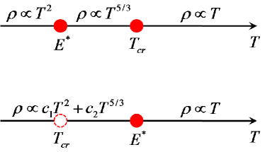
In order to make our scenario more complete, it is necessary to compare $T_{cr}$ with $E^{*}$, below which scattering with hybridization fluctuations becomes irrelevant, causing the typical Fermi-liquid behavior of electrical resistivity. $E^{*}$ is determined by the band mass of spinons and the ratio of each Fermi momentum, given by $E^{*}=\frac{0.3}{m_{f}}\Bigl{(}\frac{1-k_{F}^{c}/k_{F}^{f}}{k_{F}^{c}/k_{F}^{f}}\Bigr{)}^{3}$ KB_Indranil ; KB_Pepin . As a result, we obtain $T_{cr}>E^{*}$ in the case of $k_{F}^{c}/k_{F}^{f}>l_{c}$ while $T_{cr}<E^{*}$ in the case of $k_{F}^{c}/k_{F}^{f}<l_{c}$, where $0<l_{c}=(k_{F}^{c}/k_{F}^{f})_{c}<1$ is a constant determined by the Fermi momentum of conduction electrons. Fig. 1 shows how vertex corrections affect the temperature dependence of electrical resistivity. Our point is that although the change of the temperature dependence in the electrical resistivity is expected due to vertex corrections, the most temperature region will show the $T$-linear behavior at the Kondo breakdown quantum critical point.

Refer to caption
Figure 1: Top : When $q^{*}=k_{F}^{f}-k_{F}^{c}$ is smaller than a certain value, we obtain $T_{cr}>E^{*}$. Then, the $T$-linear resistivity turns into the $T^{5/3}$ behavior from the crossover temperature $T_{cr}$. However, the temperature regime for the $T^{5/3}$ behavior is narrow, and the most temperature region will show the $T$-linear resistivity. Down : When $q^{*}=k_{F}^{f}-k_{F}^{c}$ is larger than a certain value, we obtain $T_{cr}<E^{*}$. Then, the $T$-linear resistivity changes into $\rho\propto c_{1}T^{2}+c_{2}T^{5/3}$, where $c_{1}$ and $c_{2}$ are positive numerical constants, difficult to determine with confidence in this study.

It is interesting to notice that the Hall coefficient is not renormalized due to interactions. It remains as the Fermi-liquid value, resulting from conduction electrons only. We argue that the non-renormalization of the Hall coefficient justifies our calculation based on the quantum Boltzmann equation approach.

IV Summary

In this paper we claim that vertex corrections associated with hybridization fluctuations are relevant in electrical transport. Such corrections turn out to change the $T$-linear resistivity into $T^{5/3}$ at the Kondo breakdown quantum critical point. However, we find that the crossover temperature is too low to clarify the regime of the $T^{5/3}$ behavior experimentally. In other words, the $T$-linear resistivity will be observed in a wide range of temperatures at the Kondo breakdown quantum critical point. We justify our approximation scheme in the quantum Boltzmann equation approach, based on the fact that the Hall coefficient is not renormalized by interactions because the Hall conductivity is renormalized in the same way as the longitudinal conductivity.

We would like to close our paper, discussing the structure of our quantum Boltzmann equation approach. An essential approximation is that two bosonic degrees of freedom, hybridization and gauge fluctuations, are in equilibrium. In principle, this approximation is not consistent with fermion dynamics out of equilibrium because such bosonic excitations originate from complex textures of interacting fermions Maslov . A more complete treatment will be to start from two coupled quantum Boltzmann equations derived from the fermion-only model after integrating over both hybridization and gauge fluctuations. However, the time scale for bosons to relax into equilibrium may be much shorter than that of fermions, justifying the present approximation. Of course, this is not an easy problem, pursued in the future. In addition, our quantum Boltzmann equation approach seems to take ladder-type vertex corrections in the two-band model. Recall that the quantum Boltzmann equation approach in the one-band model introduces the ladder type of vertex corrections, making the Ward identity satisfied when the fermion self-energy is evaluated in the Eliashberg approximation YB_QBE . It will be an interesting problem to identify relevant diagrams for our vertex corrections in electrical transport coefficients.

This work was supported by the National Research Foundation of Korea (NRF) grant funded by the Korea government (MEST) (No. 2011-0074542).

References

  • (1) H. v. Lohneysen, A. Rosch, M. Vojta, and P. Wolfle, Rev. Mod. Phys. 79, 1015 (2007); P. Gegenwart, Q. Si, and F. Steglich, Nature Physics 4, 186 (2008).
  • (2) J. Custers, P. Gegenwart, H. Wilhelm, K. Neumaier, Y. Tokiwa, O. Trovarelli, C. Geibel, F. Steglich, C. Pepin, and P. Coleman, Nature 424, 524 (2003).
  • (3) A. Rosch, A. SchrΓΆder, O. Stockert, and H. v. LΓΆhneysen, Phys. Rev. Lett. 79, 159 (1997).
  • (4) J. Rech, C. PΓ©pin, and A. V. Chubukov, Phys. Rev. B 74, 195126 (2006).
  • (5) Ar. Abanov and A. Chubukov, Phys. Rev. Lett. 93, 255702 (2004).
  • (6) R. Kuchler, N. Oeschler, P. Gegenwart, T. Cichorek, K. Neumaier, O. Tegus, C. Geibel, J. A. Mydosh, F. Steglich, L. Zhu, and Q. Si, Phys. Rev. Lett. 91, 066405 (2003).
  • (7) L. Zhu, M. Garst, A. Rosch, and Q. Si, Phys. Rev. Lett. 91, 066404 (2003).
  • (8) T. Senthil, S. Sachdev, and M. Vojta, Phys. Rev. Lett. 90, 216403 (2003); T. Senthil, M. Vojta, and S. Sachdev, Phys. Rev. B 69, 035111 (2004).
  • (9) I. Paul, C. Pepin, and M. R. Norman, Phys. Rev. Lett. 98, 026402 (2007); I. Paul, C. Pepin, M. R. Norman, Phys. Rev. B 78, 035109 (2008).
  • (10) C. Pepin, Phys. Rev. Lett. 98, 206401 (2007); C. Pepin, Phys. Rev. B 77, 245129 (2008).
  • (11) K.-S. Kim and C. PΓ©pin, Phys. Rev. Lett. 102, 156404 (2009).
  • (12) K.-S. Kim, A. Benlagra, and C. PΓ©pin, Phys. Rev. Lett. 101, 246403 (2008).
  • (13) A. Benlagra, K.-S. Kim, C. PΓ©pin, J. Phys.: Condens. Matter 23, 145601 (2011).
  • (14) Ki-Seok Kim and C. PΓ©pin, Phys. Rev. B 81, 205108 (2010); K.-S. Kim and C. PΓ©pin, Phys. Rev. B 83, 073104 (2011).
  • (15) Ki-Seok Kim, arXiv:1104.3368.
  • (16) P. A. Lee and N. Nagaosa, Phys. Rev. B 46, 5621 (1992); N. Nagaosa and P. A. Lee, Phys. Rev. Lett. 64, 2450 (1990).
  • (17) K.-S. Kim, C. PΓ©pin, J. Phys.: Condens. Matter 22, 025601 (2010).
  • (18) Y.-B. Kim, A. Furusaki, X.-G. Wen, and P. A. Lee, Phys. Rev. B 50, 17917 (1994).
  • (19) Y.-B. Kim, P. A. Lee, and X.-G. Wen, Phys. Rev. B 52, 17275 (1995).
  • (20) L. B. Ioffe and A. I. Larkin, Phys. Rev. B 39, 8988 (1989).
  • (21) D. L. Maslov, V. I. Yudson, and A. V. Chubukov, Phys. Rev. Lett. 106, 106403 (2011).