Relationship between Hubble type and spectroscopic class in local galaxies

Abstract

We compare the Hubble type and the spectroscopic class of the galaxies with spectra in SDSS/DR7. As it is long known, elliptical galaxies tend to be red whereas spiral galaxies tend to be blue, however, this relationship presents a large scatter, which we measure and quantify in detail for the first time. We compare the Automatic Spectroscopic K-means based classification (ASK) with most of the commonly used morphological classifications. Despite the degree of subjectivity involved in the morphological classifications, all of them provide consistent results. Given a spectral class, the morphological type wavers with a standard deviation between 2 and 3 $T$ types, and the same large dispersion characterizes the variability of spectral classes fixed the morphological type. The distributions of Hubble types given an ASK class are very skewed – they present long tails that go to the late morphological types for the red galaxies, and to the early morphological types for the blue spectroscopic classes. The scatter is not produced by problems in the classification, and it remains when particular subsets are considered – low and high galaxy masses, low and high density environments, barred and non-barred galaxies, edge-on galaxies, small and large galaxies, or when a volume limited sample is considered. A considerable fraction of the red galaxies are spirals (40–60%), but they never present very late Hubble types (Sd or later). Even though red spectra are not associated with ellipticals, most ellipticals do have red spectra: 97% of the ellipticals in the morphological catalog by Nair & Abraham, used here for reference, belong to ASK 0, 2 or 3. It contains only a 3% of blue ellipticals. The galaxies in the green valley class (ASK 5) are mostly spirals, and the AGN class (ASK 6) presents a large scatter of Hubble types from E to Sd. We investigate variations with redshift using a volume limited subsample mainly formed by luminous red galaxies. From redshift $0.25$ to now the galaxies redden from ASK 2 to ASK 0, as expected from the passive evolution of their stellar populations. Two of the ASK classes (1 and 4) gather edge-on spirals, and they may be useful in studies requiring knowing the intrinsic shape of a galaxy (e.g., weak lensing calibration).

1. Introduction

It is long known how the Hubble sequence correlates with the colors of the galaxies. Ellipticals tend to be red whereas spirals tend to be blue (e.g., Hubble 1936; Humason 1931; Morgan & Mayall 1957; Aaronson 1978; Bershady 1995; Zaritsky et al. 1995). It is also well known that the relationship is far from being one-to-one (e.g. Connolly et al. 1995; Sodre & Cuevas 1997; Formiggini & Brosch 2004; Ferrarese 2006). There are red spiral galaxies (e.g., van den Bergh 1976; Dressler et al. 1999; Deng et al. 2009; Masters et al. 2010a), as well as blue ellipticals (e.g., Deng et al. 2009; Schawinski et al. 2009; Kannappan et al. 2009; Huertas-Company et al. 2010). The correlation changes with time, and some morphologies now rare were not unusual early on (e.g., Reshetnikov et al. 2003; Elmegreen & Elmegreen 2005). Blue galaxies become more common as the universe gets younger (e.g., Lilly et al. 1995; Madau et al. 1996; Delgado-Serrano et al. 2010), even though many ellipticals and spirals were already in place at high redshift (e.g., van den Bergh 2002; Aguerri & Trujillo 2002; Trujillo & Aguerri 2004). The relationship gets fuzzier with increasing lookback time, to perhaps disappear in the early universe (Conselice 2006; Huertas-Company et al. 2009).

In principle, the origin of the relationship between spectrum and morphology is relatively well understood. Ellipticals formed their stars long ago, therefore, their stellar populations are aged and so red. Spirals are still forming stars, and massive young stars that are blue contribute significantly to the integrated galaxy spectrum. The details of the relationship are not so clear, though. It remains unknown why local galaxies are grouped into two main colors (e.g., Strateva et al. 2001; Blanton et al. 2003; Blanton & Moustakas 2009) while their shapes follow a continuous distribution of Hubble types. The reasons for having outliers from the main relationship are even more unclear. Do outliers represent unusual galaxies living outside the main stream, or are they transients during the regular galaxy evolution? Galaxies evolve in spectrum and in shape during their lifetimes, but we ignore whether the morphological changes lead or trail the spectral changes.

The advent of new data sets allows us characterizing the relationship between Hubble type and spectroscopic class with unprecedented detail. This is the purpose of our work. We compare the spectroscopic classification by Sánchez Almeida et al. (2010) with various morphological catalogs existing in the literature (de Vaucouleurs et al. 1991; Kennicutt 1992; Fukugita et al. 2007; Nair & Abraham 2010; Lintott et al. 2010; Huertas-Company et al. 2011). The Automatic Spectroscopic K-mean-based classification by Sánchez Almeida et al., ASK, comprises the $\sim 10^{6}$ galaxies with spectra in Sloan Digital Sky Survey Data Release seven (SDSS/DR7, Stoughton et al. 2002; Abazajian et al. 2009). We use ASK because it provides a comprehensive description of all the spectral types existing in nearby galaxies. It is finer than other alternatives involving large data sets (e.g., principal component analysis, Yip et al. 2004), and the option of using color cuts and line ratios would require additional work to assess the completeness of the approach. In the vein of all previous studies comparing spectroscopic and morphological classifications, we find a general trend with large scatter. The work describes and quantifies such relationship, as a constraint to be used elsewhere to test galaxy evolution theories.

The paper is organized as follows: § 2 introduces the spectral classification to make the paper comprehensive. The empirical comparison between spectral classes (spectro-class) and Hubble types (morpho-types) is carried out in § 3. We use the catalog by Nair & Abraham (2010) as reference since it provides an optimal compromise between enough galaxies and detailed morphological types (§ 3.1), however, many of the morphological catalogs commonly used are analyzed as well (§ 3.2 Fukugita et al. 2007; § 3.3 de Vaucouleurs et al. 1991; § 3.4 Huertas-Company et al. 2011; § 3.5 Lintott et al. 2010; and § 3.6 Kennicutt 1992). The morphological classifications have a large degree of subjectivity. The hazy logic behind the human pattern recognition skills is responsible for the types, either directly, or through training sets in machine learning automatic procedures. In order to be more quantitative, we try to compare the ASK classes with morphologically related parameters that can be measured directly from galaxy images (§ 4), and which have been used in the so-called quantitative morphology (see, e.g., Odewahn et al. 2002; de la Calleja & Fuentes 2004; Conselice 2006). Possible variations with redshift of the color-shape relationship are briefly considered in § 5. The results are analyzed and summarized in § 6. Distances and look-back times are based on a Hubble constant $H_{0}=70$ km sec^-1 Mpc^-1. All our galaxies have redshifts $\leq 0.25$.

2. The ASK spectral classification

The ASK spectral classification is detailed in Sánchez Almeida et al. (2010). For the sake comprehensiveness, however, this section summarizes its main properties. ASK considers all the galaxies with spectra in SDSS/DR7. Those with redshift smaller than 0.25 are transformed to a common rest-frame wavelength scale, and then re-normalized to the integrated flux in the SDSS $g$-filter. These two are the only manipulations the spectra undergo before classification. We wanted the classification to be driven only by the shape of the visible spectrum (from 400 to 770 nm), and these two corrections remove obvious undesired dependencies of the observed spectra on redshift and galaxy apparent magnitude. We deliberately avoid correcting for other effects requiring modeling and assumptions (e.g., dust extinction, seeing, or aperture effects). This approach is in the spirit of the rules for a good classification put forward by Sandage (2005), where he points out that physics must not drive a classification. Otherwise the arguments become circular when the classification is used to drive physics. Obviously this approach does not imply disregarding the fairly complete understanding of galaxy physics we have today. It just separates the interpretation of the spectra from determining their observed shapes. The employed classification algorithm, k-means, is a robust workhorse that makes it doable the simultaneous classification of the full data set. It is commonly employed in data mining, machine learning, and artificial intelligence (e.g., Everitt 1995; Bishop 2006), and it guarantees that similar rest-frame spectra belong to the same class. 99% of the galaxies can be assigned to only 17 major classes, with 11 additional minor classes including the remaining 1%. It is unclear whether the ASK classes represent genuine clusters in the 1637-dimensional classification space, or if they partake a continuous distribution – probably the two kinds of classes are present (see Sánchez Almeida et al. 2010; Ascasibar & Sánchez Almeida 2011). All the galaxies in a class have very similar spectra, which are also similar to the class template spectrum formed as the average of all the spectra of the galaxies in the class. These template spectra vary smoothly and continuously. They were labeled according to the $u-g$ color, from the reddest, ASK 0, to the bluest, ASK 27. The use of numbers to label the classes does not implicitly assumes the spectra to follow a one dimensional family. The numbers only name the classes. The sorting (and, so, the naming) would have been slightly different using other bandpasses to define colors. In general, however, the smaller the ASK class the redder the full spectrum, and we often use the terms red and blue referring to low and high ASK numbers, respectively. The ASK classification of all the galaxies with spectra in SDSS/DR7 is publicly available. In this paper we only employ the $\sim 7\cdot 10^{5}$ SDSS/DR7 galaxies having redshifts $\leq 0.25$.

3. Morphological type versus spectroscopic class

Eyeball morphological classifications are based on factors like the presence or not of a disk, the bulge-to-disk ratio, the presence of arms, their organization, and so on. Obviously, they entail a significant degree of subjectivity. In order to evaluate the effect of this source of error on the relationship between morphological type and spectroscopic class, we use a number of different classifications. They are not homogeneous, having diverse finesse and, therefore, based on slightly different criteria – e.g., Nair & Abraham (2010) employ 14 types whereas Lintott et al. (2010) divide all galaxies into only two bins, ellipticals and spirals. Following Table 1 in Nair & Abraham (2010), our Table 1 provides a rough equivalence between the different morphological classifications employed here. The classical Third Reference Catalog by de Vaucouleurs et al. (1991, RC3) is used as guide in Table 1. The criteria that define the types in this catalog are summarized in § 3.3, where we employ RC3 to provide the morphological types.

Table 1Equivalence between the different morphological classification schemes used in the work

	c0	E0	E+	S0-	S0	S0+	S0/a	Sa	Sab	Sb	Sbc	Sc	Scd	Sd	Sdm	Sm	Im
de Vaucouleurs et al. (1991)	-6	-5	-4	-3	-2	-1	0	1	2	3	4	5	6	7	8	9	10
Fukugita et al. (2007)	E	E	E	S0	S0	S0	S0	Sa	Sa	Sb	Sb	Sc	Sc	Sd	Sd	Im	Im
Nair & Abraham (2010)	E	E	E	ES0	S0	S0	S0a	Sa	Sab	Sb	Sbc	Sc	Scd	Sd	Sdm	Sm	Im
Huertas-Company et al. (2011)	E	E	E	E	S0	S0	S0	Sab	Sab	Sab	Scd	Scd	Scd	Scd	Scd	Scd	Scd
Lintott et al. (2010)	E	E	E	Sp	Sp	Sp	Sp	Sp	Sp	Sp	Sp	Sp	Sp	Sp	Sp	Sp	Sp

Note. — The table has been adapted from Nair & Abraham (2010), Table 1. The classification in the first row is not used here, but it remains as in the original table for cross-reference.

3.1. Hubble types derived by Nair & Abraham (2010)

The morphological classification by Nair & Abraham (2010) serves as reference. Although all the analyzed classifications provide consistent results, the one by Nair & Abraham is selected for in-depth study because it represents the best compromise between volume and finesse. It contains 14034 galaxies, distinguishes between 14 morphological types (see Table 1), and contains additional information like the presence of bars, or the galaxy environment. In addition, the classification by Nair & Abraham is almost magnitude limited, therefore, it can be employed to model the results corresponding to a volume limited sample. The classification considers all the galaxies in SDSS/DR4 with $g<16$ and redshift $\leq 0.1$. The redshift upper limit removes almost no galaxy from the original pool therefore, in practice, the sample is apparent magnitude limited.

Figure 1a shows the scatter plot of Hubble type vs ASK class for all the galaxies in Nair & Abraham (2010). As we will do throughout the work, we have added some random noise (normally distributed, 0.3 classes standard deviation) to the actual positions of the galaxies. The sampling in Hubble type and ASK class is discrete and so coarse that, unless noise is added, the galaxies overlap not showing up in scatter plots. The first obvious result drawn from inspecting Fig. 1a is the dispersion of ASK classes fixed the morphological type, and vice versa. Such dispersion exceeds the uncertainty in Hubble type ($\leq 0.5$ types – Nair & Abraham 2010) and ASK class ($<1$ class – Sánchez Almeida et al. 2010). In order to quantify the dispersion, we make use of the two dimensional histogram $N(A,T)$, with $A$ the ASK class, and $T$ the Hubble type. We characterize the properties of the observed distribution using the first moments of the two marginal distribution functions that result from integrating over one of the two variables. Namely, given a class $A$, we calculate the mean $T$ type, $\mu_{T}(A)$,

$$\mu_{T}(A)=N^{-1}_{T}(A)\,\sum_{i}T_{i}\,N(A,T_{i}),$$ (1)

the standard deviation, $\sigma_{T}(A)$,

$$\sigma^{2}_{T}(A)=N^{-1}_{T}(A)\,\sum_{i}\big{[}T_{i}-\mu_{T}(A)\big{]}^{2}\,N(A,T_{i}),$$ (2)

the skewness, $\beta_{T}(A)$,

$$\beta_{T}(A)=N^{-1}_{T}(A)\,\sum_{i}\big{\{}\big{[}T_{i}-\mu_{T}(A)\big{]}/\sigma_{T}(A)\big{\}}^{3}\,N(A,T_{i}),$$ (3)

and the kurtosis${}^{\ref{def_kur}}$, $\kappa_{T}(A)$,

$$\kappa_{T}(A)=N^{-1}_{T}(A)\,\sum_{i}\big{\{}\big{[}T_{i}-\mu_{T}(A)\big{]}/\sigma_{T}(A)\big{\}}^{4}\,N(A,T_{i})-3.$$ (4)

The sums are over all $T$ types given an $A$ class, and the symbol $N_{T}(A)=\sum_{i}\,N(A,T_{i})$ stands for the total number of galaxies belonging to class $A$. We also compute the statistical parameters for the dispersion among the ASK classes given a $T$ type. They are formally identical to the previous definitions but exchanging $A$ with $T$, i.e., $\mu_{A}(T),\sigma_{A}(T),\beta_{A}(T)$ and $\kappa_{A}(T)$. Tables 2 and 3 list all these statistical parameters plus the median (type that splits the sample into two halves) and the mode (most probable value). Note than one can approximately retrieve the full distribution from these few moments (e.g., Martin 1971). The tables include the values corresponding to the full set of Nair & Abraham galaxies, as well as those corresponding to subsets analyzed below. The symbols in Figs. 1b and 1c represent $\mu_{T}(A)$ and $\mu_{A}(T)$, respectively. These figures also include as shaded areas the regions around the median containing 68% (dark gray) and 95% (light gray) of the galaxies. Several results stand out. There is a general trend for the red galaxies to have early morphological types, and for the blue galaxies to have late morphological types, as quantified in Figs. 1b and 1c. However, the relationship has a large scatter with a standard deviation between 2 and 3 types, both for the dispersion of Hubble types given an ASK class, and for the dispersion of spectroscopic classes fixed the Hubble type (see columns labeled Stand. Dev. in Tables 2 and 3). Figure 2 shows galaxy images that illustrate the various parts of the scatter plot – the main trend along the diagonal, as well as the outliers represented by red spirals (upper left) and blue ellipticals (bottom right). The distributions of Hubble types given the ASK class are very skewed; they present extended tails that go to the late morphological types for the red galaxies, and to the early morphological types for the blue spectroscopic classes. A notable fact is the lack of Sd, Sdm, Im and Sm in ASK classes with red spectra. The opposite is not true: ellipticals with emission lines and very blue spectra are not very common, but they do exist.

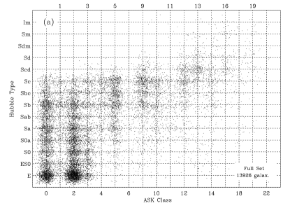
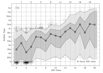
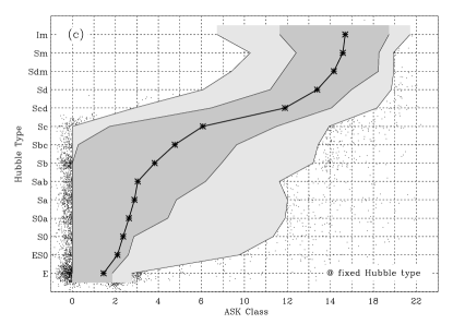
Figure 1.— Hubble type vs ASK class for the full set of galaxies in Nair & Abraham (2010). (a) Scatter plot with small noise added to avoid overlapping. (b) Average Hubble type given an ASK class (the square symbols), and regions containing 68% of the galaxies (the dark shaded area) and 95% of the galaxies (the light shaded area). (c) Average ASK class given a Hubble type (the asterisks), and regions containing 68% and 95% of the galaxies. Abscisae include only major ASK classes.

Table 2Statistical parameters characterizing the dispersion of Hubble types given an ASK class.

ASK	Mean			Median			Mode			Stand. Dev.			Skewness			Kurtosis
0	S0a$-0.1$	Sa$-0.4$	S0$+0.2$	S0a	Sa	ES0	E	E	E	2.6	2.7	2.4	0.3	0.1	0.8	-1.2	-1.2	-0.8
1	Sa$+0.5$	Sab$+0.4$	S0$+0.3$	Sab	Sb	ES0	Sb	Sb	E	2.5	2.3	2.4	-0.4	-0.6	1.0	-1.0	-0.2	-0.1
2	S0$+0.2$	S0a$-0.5$	S0$-0.1$	S0	S0	ES0	E	E	E	2.4	2.2	2.3	0.8	0.7	1.0	-0.6	-0.2	-0.2
3	Sa$-0.4$	Sa$-0.4$	S0a$+0.4$	S0a	S0a	S0a	E	ES0	E	2.7	2.8	2.7	0.3	0.5	0.4	-1.2	-1.1	-1.2
4	Sb$-0.0$	Sb$+0.2$	Sab$+0.3$	Sb	Sbc	Sb	Sc	Sc	Sb	2.0	2.1	2.1	-0.7	-0.6	-0.4	0.1	-0.5	0.0
5	Sb$-0.1$	Sb$+0.1$	Sb$-0.4$	Sb	Sbc	Sb	Sb	Sc	Sb	2.0	2.2	2.0	-0.8	-0.8	-0.8	0.0	-0.2	-0.1
6	Sab$+0.1$	Sab$-0.2$	Sab$-0.1$	Sb	Sab	Sb	Sb	Sa	Sb	2.0	2.0	2.0	-0.6	-0.2	-0.6	-0.5	-0.9	-0.5
7	Sab$-0.4$	Sa$-0.4$	Sab$-0.4$	Sa	S0a	Sa	S0a	S0a	S0a	2.0	1.6	2.0	0.2	1.2	0.1	-1.1	1.4	-1.1
8	Sab$-0.3$	—	Sab$+0.3$	Sa	—	Sa	Sa	—	Sa	1.9	—	1.9	1.0	—	0.7	-0.8	—	-1.5
9	Sbc$-0.3$	Sbc$+0.4$	Sb$+0.5$	Sbc	Sc	Sbc	Sc	Sc	Sc	2.0	2.0	2.0	-1.1	-1.4	-1.1	1.2	2.3	1.0
10	Sb$+0.3$	Sb$+0.5$	Sb$-0.1$	Sbc	Sbc	Sb	Sc	Sc	Sb	2.1	2.4	2.0	-0.5	-0.6	-0.5	0.3	0.1	0.3
11	Sb$-0.1$	Sb$-0.3$	Sb$-0.4$	Sb	Sb	Sb	Sc	Sc	Sb	2.1	2.7	2.0	-0.2	0.0	-0.3	0.5	0.1	0.3
12	Sbc$+0.2$	Sc$+0.1$	Sbc$-0.1$	Sc	Scd	Sbc	Sc	Scd	Sc	2.1	1.8	2.1	-0.9	-1.5	-0.7	0.8	2.5	0.5
13	Sc$+0.1$	Scd$-0.2$	Sc$-0.2$	Scd	Scd	Scd	Scd	Scd	Scd	2.5	1.9	2.7	-1.4	-1.9	-1.2	1.9	6.4	1.1
14	Sbc$+0.1$	Sbc$+0.1$	Sbc$-0.2$	Sc	Sc	Sbc	Sc	Sc	Sc	2.5	2.9	2.6	-0.6	-0.6	-0.5	0.6	0.1	0.4
16	Scd$-0.0$	Scd$+0.4$	Scd$-0.3$	Scd	Sd	Scd	Scd	Sd	Scd	2.4	2.5	2.6	-1.1	-1.2	-1.0	1.9	1.7	1.1
18	Sbc$+0.0$	Sbc$-0.2$	Sb$+0.5$	Sc	Sbc	Sbc	Sc	Sd	Sc	3.1	3.1	3.3	-0.4	-0.3	-0.2	-0.7	-1.0	-0.9
19	Scd$+0.1$	Sd$-0.4$	Scd$-0.4$	Sd	Sd	Sd	Scd	Scd	Sm	2.9	2.5	3.5	-1.0	-1.2	-0.8	0.4	1.5	-0.6
22	Scd$-0.1$	Scd$-0.4$	Sbc$+0.3$	Sd	Scd	Scd	Sd	Scd	E	3.9	3.6	4.6	-1.0	-0.7	-0.3	-0.0	-0.8	-1.4
23	Sd$+0.1$	Sd$-0.2$	Sd$-0.2$	Sm	Sdm	Sm	Sm	Sm	Sm	3.5	3.2	4.1	-1.6	-1.4	-1.3	1.2	0.9	0.1
26	Sc$+0.0$	Sc$+0.1$	—	Scd	Scd	—	Sa	Scd	—	2.9	2.8	—	-0.5	-0.6	—	-1.5	-1.3	—

.

Note. — Morphological types from Nair & Abraham (2010). ASK classes not included imply having no enough galaxies in the bin to compute statistical properties. Hubble types are coded in Table 1

Table 3Statistical parameters characterizing the dispersion of ASK classes once the Hubble type is fixed.

Hubble Type	Mean			Median			Mode			Stand. Dev.			Skewness			Kurtosis
E	1.5	2.3	1.5	2	2	2	2	2	2	1.4	2.7	1.4	2.7	2.7	2.7	21.0	8.1	21.2
ES0	2.1	3.0	2.1	2	2	2	2	2	2	2.2	2.8	2.2	2.4	2.4	2.4	8.1	5.6	8.2
S0	2.4	3.2	2.5	2	2	2	2	2	2	2.5	3.2	2.6	2.2	1.9	2.1	6.1	3.4	5.5
S0a	2.6	4.2	2.9	2	3	2	2	2	2	2.9	4.2	3.1	1.7	1.31	1.6	3.1	0.7	2.3
Sa	2.9	5.0	3.6	2	3	2	0	2	2	3.1	4.6	3.3	1.5	0.9	1.1	2.0	-0.4	0.8
Sab	3.0	4.3	3.6	2	3	2	0	0	2	3.1	3.8	3.2	1.1	0.8	0.9	0.6	-0.1	-0.0
Sb	3.8	5.2	4.6	3	5	5	0	0	2	3.4	4.0	3.5	0.8	0.5	0.5	-0.2	-0.9	-0.5
Sbc	4.8	6.3	5.4	5	9	5	5	9	5	3.4	4.0	3.3	0.4	0.2	0.2	-0.5	-0.9	-0.6
Sc	6.1	9.1	8.8	9	9	9	9	9	9	3.5	3.8	3.3	0.1	-0.1	-0.1	-0.7	-0.8	-0.6
Scd	11.9	12.4	12.2	12	13	13	13	13	13	2.8	2.6	2.5	-0.6	-0.6	-0.8	0.1	0.9	0.8
Sd	13.4	13.8	13.3	13	14	13	13	13	13	2.5	2.4	2.5	-0.9	-1.2	-1.3	1.8	3.0	3.2
Sdm	14.2	15.7	14.0	14	14	14	13	13	13	2.0	2.0	1.9	-0.0	0.2	0.0	-0.7	-1.1	-0.4
Sm	15.6	16.1	15.5	16	16	16	16	16	16	2.0	1.7	2.0	-1.3	-0.5	-1.3	4.3	0.2	4.3
Im	15.7	16.2	14.2	16	16	16	16	16	16	2.5	2.1	2.6	-0.7	-0.8	-0.6	-0.4	0.9	-0.5

Note. — Morphological types from Nair & Abraham (2010). Only major ASK classes are considered to compute the statistical parameters.

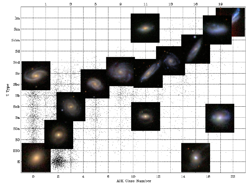
Figure 2.— Scatter plot of Hubble type versus ASK class for the galaxies classified by Nair & Abraham (2010) (same as Fig. 1a). In addition, we overplot SDSS images of representative galaxies located at various places on the diagram. Note the trend from red early types, to blue late types, roughly following the diagonal of the diagram. On top of it, however, there is a large scatter produced by red spirals (e.g., Sc & ASK 0), and blue ellipticals (e.g., E & ASK 16). Only the upper left corner of the diagram is truly devoid of targets, which would correspond to (non-existing) red Sd, Sdm, Im and Sm galaxies.

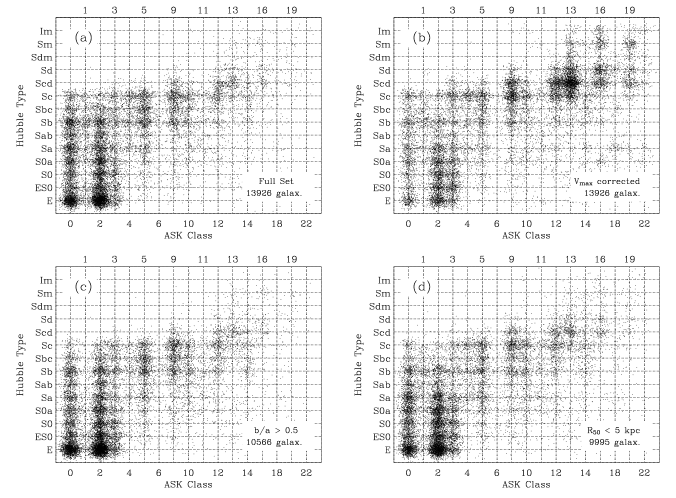
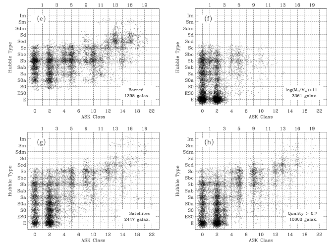
Figure 3.— Scatter plots of Hubble type versus ASK class for galaxies in Nair & Abraham (2010). (a) Same as Fig. 1a. All the other panels represent trims on this galaxy set. (b) Full set corrected so that, rather than a magnitude limited sample, it represents a volume limited sample. (c) Only rounded galaxies are included, which removes edge-on disk galaxies. See how ASK 1 and 4 have been greatly reduced as compared to (a). (d) Small galaxies, with half-light radius $R_{50}<5~{}$kpc. (e) Only galaxies labeled as barred. (f) High mass galaxies (stellar mass $M_{\star}>10^{11}\,M_{\odot}$). Blue types are gone, ellipticals are greatly reinforced, and the relative number of ASK 0 galaxies has also increased. (g) Satellite galaxies. They are tracing high density environments. (h) Only galaxies with high confidence ASK classification. All plots contain the same number of points, but the insets at the bottom right corners give the number of galaxies left by the particular selection (see the main text for details). Only major ASK classes are included.

The scatter shown in Figs. 1, and quantified in Tables 2 and 3, has been inferred from the particular sample of galaxies selected by Nair & Abraham (2010). However, with small modifications, it is representative of the relationship and scatter existing among local galaxies. One can support this claim by comparing the results with those obtained using other morphological catalogs, an approach to be pursued in the forthcoming subsections. In addition, the catalog by Nair & Abraham (2010) is large enough to be partaken, thus allowing the analysis of whether the relationship depends on particular properties of the galaxy sample. The rest of the section is devoted to such exercise. We have constructed scatter plots Hubble-type-vs-ASK-class using subsets of Nair & Abraham galaxies. Some of them are shown in Fig. 3. Obviously, re-sampling the original set reduces the number of galaxies, which makes it difficult to visually compare different scatter plots. In order avoid this unwanted dependence, we show the same number of galaxies in all plots. They are not real galaxies but points randomly drawn from the histograms inferred from the real galaxies. The number of real galaxies left by the selection is given in the inset of the corresponding panel. Figure 3a shows the scatter plot of the original distribution and it is included for reference. (It is equivalent to Fig. 1a.) Figure 3b shows the scatter plot in the case that the sample were volume limited, i.e., if it would include all galaxies within a fixed volume. We have used the $V_{\rm max}$ approach to construct the sample, as explained in appendix A. The importance of the blue galaxies has increased with respect to Fig. 3a because intrinsically faint galaxies are underrepresented in magnitude limited samples (Malmquist bias), and many of them tend to be blue (e.g., Balogh et al. 2004; Blanton & Moustakas 2009). However, the original dispersion remains. This fact is quantitatively corroborated in Tables 2 and 3; compare the standard deviations in columns $(a)$ and $(b)$. Figure 3c shows the scatter plot for rounded targets, which excludes edge-on disk galaxies. Explicitly, we show galaxies where the ratio between the minor and major axes $b/a>0.5$. The scatter remains, although the density of red late type galaxies is somehow reduced. This can be better appreciated in Fig. 4, the thick lines, which portrays histograms of ASK 2 galaxies for various aspect ratios – the shape of the distribution remains, but with a slight relative increase of E-S0 galaxies with increasing $b/a$ threshold.

Figure 4.— Histograms of Hubble types for galaxies of different ellipticities $b/a$; from the full range of possible values ($b/a>0,$ the solid lines) to more rounded galaxies ($b/a>0.5$, the dashed lines, and $b/a>0.8$, the dotted lines). The thick and thin lines represent ASK 2 and ASK 1 galaxies, respectively. Note how ASK 1 galaxies tend to disappear with increasing $b/a$, meaning that they mostly are edge-on (disk) systems. The axis-ratio threshold has almost no effect on ASK 2, except for a slight increase of early types when considering rounded galaxies. The histograms are normalized to the total number of galaxies, i.e., galaxies of all ASK classes and Hubble types.

Part of the red spirals are edge-on galaxies, which are known to be reddened with respect to their face-on counterparts (e.g., Giovanelli et al. 1994; Masters et al. 2010b, and § 6). However, not all the red spirals are edge-on systems (see Figs. 2, 3c and 4, as well as Masters et al. 2010a). Note also that most galaxies corresponding to ASK 1 and 4 have disappeared from Fig. 3c, indicating that these classes seem to be preferentially formed by edge-on spirals. This drastic decrease is also illustrated in Fig. 4, where the thin lines show how the relative number of ASK 1 galaxies drops down when selecting only rounded galaxies. (ASK 4 galaxies behave similarly.) The columns $(c)$ in Tables 2 and 3 show the statistical parameters for these face-on systems, which are not very different from those of the original sample, listed in columns $(a)$. Figure 3d shows the scatter plot considering only small galaxies, namely galaxies with half-light radius $R_{50}<5\,$kpc. SDSS spectra are obtained with a 3 arcsec fiber, which covers only the central parts of the large galaxies. Statistically, small galaxies look small on the sky, therefore, the fact that small galaxies show a scatter similar to the full sample indicates that red spirals are not artificially produced by the fiber covering only the central (red) bulge, since this effect would preferentially affect large galaxies. Obviously, the above argument would be stronger using angular sizes rather than physical sizes, but we consider it sufficient because comparisons made with the other morphological catalogs using the proper angular sizes also discard the bias (see § 3.2 and 4). Figure 3e shows the scatter plot for barred galaxies (i.e., flagged as strong or intermediate barred in Nair & Abraham 2010). Ellipticals have disappeared since bars are associated with disks in galaxies (e.g., Méndez-Abreu et al. 2010), and this lack of ellipticals reduces the scatter of the plot in the region ASK 0–3. Barred S0 galaxies are also rare in Fig. 3e, which was expected in view of the known shortage of bars in S0s (see, e.g., Barazza et al. 2008; Aguerri et al. 2009; Buta et al. 2010). Figure 3f shows the scatter plot for massive galaxies with stellar masses $M_{\star}>10^{11}\,M_{\odot}$. Only red classes remain. (Massive galaxies tend to be red, even if they are spirals; see, Blanton & Moustakas 2009 and references therein.) ASK 0 results particularly enhanced independently of whether they are elliptical or spirals. Note that ASK 12 and bluer classes do not seem to be associated with massive galaxies. All these properties are more clearly illustrated by the solid lines in Fig. 5, which are just projections of Fig. 3f in ordinates (Fig. 5a) and abscissae (Fig. 5b). For comparison, Fig. 5 also shows the histograms for low mass galaxies ($M_{\star}<10^{9.5}\,M_{\odot}$; the dashed lines). In contrast with high mass galaxies, low mass galaxies tend to be blue (ASK 12 and larger), and have late Hubble types (Sc and later), although, low mass galaxies of all colors and morphologies exist.

Figure 5.— (a) Distribution of Hubble types among the massive galaxies (stellar mass $M_{\star}>10^{11}\,M_{\odot}$, the solid line) and the low mass galaxies ($M_{\star}<10^{9.5}\,M_{\odot}$, the dashed line) in the catalog by Nair & Abraham (2010). (b) Distribution of ASK classes for the same two sets of galaxies. All histograms are normalized to one.

The catalog by Nair & Abraham (2010) contains a flag indicating if the galaxy is or not the most luminous of its group. Figure 3g represents those that are not, i.e., those marked as satellite galaxies. The scatter remains indicating that the presence of companion galaxies (and thus of interaction) does not significantly modifies the diagram. However, there is a subtle difference with respect to Fig. 3a, namely, an excess of S0 and latter types with respect to the ellipticals. This preference is also known to be attributable to high density environments. Finally, Fig. 3h shows that the scatter is not produced by spectral misclassifications. It shows galaxies with high ASK quality, specifically, with a probability of belonging to its class larger than 70% – see Sánchez Almeida et al. (2010) for details on the definition of quality. This high quality subset represents 78% of the Nair & Abraham sample.

Figure 6 contains the percentage of late type galaxies in each ASK class. It shows how spirals are present in all spectral classes. Obviously they dominate the blue ASK classes (4 and bluer), but their contribution is not negligible even in the red ASK 0, 2 and 3 that are characteristic of ellipticals. For example, in the original sample of Nair & Abraham (2010), 57% of the red ASK 0, 2 and 3 are formed by spirals (S0 and later). The actual fraction depends on the used sample (see Fig. 6), but red spirals turn out to be common.

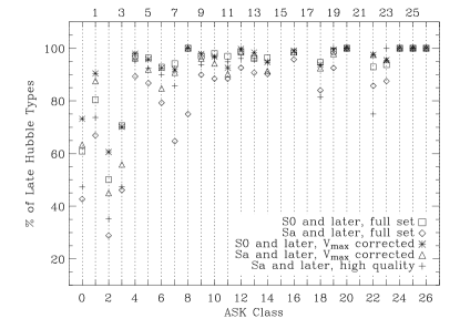
Figure 6.— Percentage of late Hubble types corresponding to each ASK class. Late types dominate the blue classes, but they are also very common among red spectra. The different symbols represent various galaxy samples, as indicated in the inset. The squares correspond to the full Nair & Abraham (2010) data set when late type means S0 and later. The rhombi also correspond to the same original data for Sa galaxies and later. The asterisks and triangles consider a volume limited sample. Finally, the plus signs correspond to the original data set removing galaxies with uncertain ASK classes.

Based on Figs. 1, 2, 3, 4, 5, and 6, Tables 2 and 3, as well as on additional explorations, we distill the following results (sorted not necessarily according to importance):

• We recover the well known global trend indicating that early Hubble types tend to be red and late Hubble types tend to be blue. This trend presents a large scatter which has been quantified in Tables 2 and 3. Given a Hubble type, the ASK class varies with a standard deviation between 2 and 3 classes. The same happens with the Hubble type once the ASK class is fixed.

• The scatter is real (see Fig. 2). It is not produced by problems in the classification, and it is not reduced when particular subsets are considered – low and high galaxy masses, low and high density environments, barred and non-barred galaxies, face-on galaxies, small and large galaxies, or even when a volume limited sample is considered.

• The upper left corner of the scatter plots is empty. There are no Sd, Sdm, Sm or Im galaxies with red spectra. This seems to indicate that morphological evolution is somewhat faster than color evolution for these morphological types (commonly associated with dwarf galaxies).

• On the contrary, there are lots of spiral galaxies in red ASK classes, suggesting that the spectrum can redden without morphological transformation, provided that the galaxy is massive enough. We find that 57% of the red ASK 0, 2 and 3 galaxies are not ellipticals (i.e., are neither E nor ES0).

• Even though red spectra are not associated with ellipticals, most ellipticals do have red spectra: 93% of the ellipticals in Nair & Abraham (2010) belong to ASK 0, 2 or 3.

• There is also a 3% of blue ellipticals (see Fig. 2), like those studied by Huertas-Company et al. (2010, see also the references in § 1).

• Low mass dwarf galaxies tend to be late type (Sc and later) and blue (ASK 12 and bluer).

• ASK 1 and 4 seem to be made of edge-on (reddened) spirals.

• All red classes contain edge-on spirals, however, not all red spirals are edge-on. The reddening associated with being edge-on may account for some of them, but not for all.

• S0s tend to be satellites, i.e., they are not the most luminous of their groups.

• Bars are not present in Es, and are almost absent in S0s.

• ASK 6 is made out of active galactic nuclei (AGN; Sánchez Almeida et al. 2010), and we find it to have a particularly flat distribution of Hubble types, going all the way from E to Sc, but not later (see Figs. 3a and 3b).

• The galaxies with transition colors are preferentially early spirals. As it is shown in Sánchez Almeida et al. (2010), ASK 5 is formed by galaxies right in the green valley and, according to Fig. 3a, 87% of them are Sa or later types. (96% are S0 or later.)

3.2. Hubble types derived by Fukugita et al. (2007)

Fukugita et al. (2007) carried out a morphological classification of bright galaxies in the north equatorial stripe of SDSS/DR3. The classification has been performed by visual inspection of SDSS $g$ images by three different observers. The catalog contains 2253 galaxies, but only 1866 galaxies have spectra, and so, ASK class. The classification comprises only six Hubble types (see Table 1), but the fact that it has been agreed by three qualified observed makes it very reliable – the mean standard deviation among the three classifications is only 0.4 types. The resulting scatter plot morpho-type vs spectro-class is presented in Fig. 7. There is no significant difference when compared to Fig. 3a. The same global trends, including the presence of red spirals and blue ellipticals, and the absence of red Sd—Im. This sample also allowed us to check that the spirals in red ASK classes remain in place even when considering rounded targets and small ($R_{50}<3$ arcsec) galaxies. Moreover, the plot is insensitive to considering or not galaxies flagged in the catalog as peculiar.

Figure 7.— Scatter plot of Hubble type vs ASK class for the SDSS/DR3 galaxies classified by Fukugita et al. (2007). In order to avoid the overlapping of galaxies with the same Hubble type and ASK class, we have added small artificial random shifts to all points. It is very similar to Fig. 3a, except that this sample contains only one tenth of the galaxies represented therein. Only major ASK classes are included.

3.3. Morphology from the 3rd reference catalog, RC3, by de Vaucouleurs et al. (1991)

The 3rd reference catalog of bright galaxies (RC3) by de Vaucouleurs et al. (1991) has been the standard for morphological classifications during the last two decades, therefore we also wanted to check the above results against this reference. For this reason, and also because their classification is finner and more precise than the others, we use it as a guide for the equivalence between different schemes (Table 1). The morphological types of RC3 are coded with $T$ types spanning from $-6$ to $+11$. Paraphrasing de Vaucouleurs (1994), the catalog includes $T$ types along the extended Hubble sequence through the four main classes E (ellipticals or spheroidals, encompassing stages T $=-6$ to T $=-4$, from compact to late), L (lenticulars or S0s, i.e. arm-less disks, T $=-3$ to T $=-1$, from early to late), Sp (spirals from S0a at T $=0$ to Sm at T $=9$ through the familiar stages a, b, c, d at T $=1,3,5,7$ with the transition types ab, bc, cd, dm at T $=2,4,6,8$), and Im (Magellanic irregulars, T $=10$, with 11 for compact).

The catalogs discussed so far are based on SDSS images, therefore, matching them with the ASK classification was trivial since SDSS targets have unique identifiers. However, this is not the case for RC3. The version of RC3 included in SDSS/DR7 just contains the right ascension and declination of the targets. In order to carry out the match, we search SDSS/DR7 for galaxies with spectra within 30 arcsec of the RC3 coordinates. We handled multiple matches by choosing the closest object. The RC3 catalog in SDSS/DR7 contains 23011 entries, with only 17801 having valid $T$ type. From them we match 3026 galaxies, which is roughly consistent with the solid angled covered by SDSS/DR7 assuming the RC3 galaxies to be evenly spread throughout the sky. The scatter plot $T$ type vs ASK class corresponding to these targets is shown in Fig. 8. It displays all the features already described in § 3.1, and we will not repeat them here. We note, however, how the presence of red spirals is even more evident than in Fig. 3a. This increase may be a bias specific to the RC3 catalog, which contains nearby galaxies, and so, galaxies of large angular size (mean half-light radius of 10″$\pm 5$″). Given the finite size of the fiber feeding the SDSS spectrograph, the bulge of the spirals contribute more with increasing apparent size, which reddens the SDSS spectra.

Figure 8.— Scatter plot of $T$ type, as given in the RC3 catalog, vs ASK class. Compare it with the reference Fig. 3a. This plot contains all the 3026 galaxies in the match we carry out. Only major ASK classes are included.

3.4. Morphology using galSVM by Huertas-Company et al. (2011)

The support vector machine procedure galSVM by Huertas-Company et al. (2008) is a machine learning algorithm which tries to find the optimal boundary between clouds of points in a high-dimensional space, even when the borders are not linear. It does not deliver a binary classification but the probability of belonging to a given class. Among other advantages, the user provides all the parameters that may be relevant for the classification, and galSVM is able to purge them and isolate only those features that are not redundant. The technique has been validated in different cases (Huertas-Company et al. 2009, 2010), and it has been recently applied by Huertas-Company et al. (2011) to classify the full set SDSS/DR7 galaxies with spectra at redshift $\leq 0.25$, i.e., exactly the data base of ASK classes used here. It requires a training set, which in this particular case was the morphological classification by Fukugita et al. (2007), studied separately in § 3.2. Huertas-Company et al. (2011) defined four wide morphological classes that include the full range of possibilities: E, S0, Sab, and Scd+Im (see Table 1). Given a galaxy, galSVM provides the probability of belonging to each one of these four types, so that the galaxy will be regarded as E if it has a large probability of being elliptical, and the same holds for the other types. The procedure classifies the $\sim 7\cdot 10^{5}$ galaxies of the dataset in only a few minutes.

Huertas-Company et al. (2011) base the classification in three observables, (1) the restframe colors ($g-r$ and $g-i$), (2) the ellipticity of the galaxy images (i.e., $b/a$ with $b$ and $a$ the minor and major axes), and (3) the concentration ($R_{90}/R_{50}$ in the SDSS $i$ filter, with $R_{\alpha}$ the radius containing $\alpha$% of the flux). The resulting scatter plot Hubble type vs ASK class is shown in Fig. 9. The correlation is clear and similar to the ones described in the previous sections.

Figure 9.— Hubble type from Huertas-Company et al. (2011) vs ASK class. The inference of Hubble type uses concentration, ellipticity and color, therefore, it is not a purely morphological classification. However, all the trends existing in Fig. 3a are also here. It contains only 20000 randomly selected points from the actual data set formed by all the $\sim 7\cdot 10^{5}$ galaxies with redshift $<0.25$ in SDSS/DR7. Only major ASK classes are included.

The similarity is to some extent surprising since the assigned Hubble types are not purely morphological. Colors were included to derive Hubble types, and yet some morpho-types do present a large color spread (typically, Sab galaxies). For reasons which remain unclear to us, the colors are regarded as unimportant by the galSVM algorithm (see § 6 for a further analysis). In order to test this conjecture, we repeated the classification in Huertas-Company et al. (2011), but only with concentration and ellipticity. The resulting scatter plot (not shown) remains similar to Fig. 9.

On top of the overall agreement, we identify two subtle differences between Fig. 9 and Fig. 3a. First, Fig. 9 clearly lacks of S0 galaxies. Somehow galSVM assigns a probability of being S0 systematically lower than that of being E, which produces the dimming of S0s when thresholding the sample with a constant probability (0.5 in the case of Fig. 9, but its value is incidental in this context). Second, the red classes ASK 1 and 4 are assigned systematically to spiral classes, even more sharply than in the previous plots. This separation results from using ellipticity as an observable for the morphological classification. In case of doubt, ASK 1 and 4 galaxies with isophotes of large eccentricity are ascribed to late morphological types. Recall that these two red classes seems to consist mostly of edge-on spirals (§ 3.1).

3.5. Morphology from Galaxy Zoo 1 (Lintott et al. 2010)

We have also compared the ASK classes with the Galaxy Zoo 1 morphological classification, where the old problem of galaxy classification has been addressed in a very original way using the current internet technology. The morpho-types are obtained by public votes of more than 100000 (non-expert) volunteers through a specially designed web interface (http://www.galaxyzoo.org). Six types are offered to the volunteers (E, clockwise Sp, counterclockwise Sp, edge-on, merger, and unknown), but this original classification is finally simplified to E, Sp and unknown (Un) after carrying out a significant bias correction to compensate for small-distant objects erroneously classified as E or Un. The Galaxy Zoo team offers a clean sample with morphologies for galaxies where, after debiasing, 80% of the votes agree. The classification is described by Lintott et al. (2008) whereas the public Galaxy Zoo release that we use is introduced in Lintott et al. (2010).

The scatter plot galaxy Zoo type vs ASK class is shown in Fig. 10b. The classification is coarser than the previous ones, but it is fully consistent with them. Figure 10a is the same as Fig. 3a, except that all types that are not ellipticals (E or ES0) have been condensed to a single class of spirals Sp. This two-class-only separation tries to mimic the galaxy Zoo classification. The similarities between Figs. 10a and 10b are more than just qualitative: 96.5% of the ellipticals in Nair & Abraham (2010) belong to ASK 0, 2 or 3, whereas the percentage is 95.0% for the clean sample in Lintott et al. (2010). Red classes ASK 0, 2 and 3 are not exclusively formed by E: 49.2% and 57% are spirals in the case of Galaxy Zoo and Nair & Abraham (2010), respectively. All the percentages mentioned above refer to the full match between ASK classes and clean Galaxy Zoo 1, which includes 247405 galaxies. In addition, the original (undebiased) Galaxy Zoo 1 classification separates between Sp and edge-on systems. It proves the existence of red face-on spirals, and how ASK 1 and 4 are formed by edge-on systems.

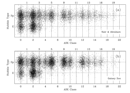
Figure 10.— Comparison between the scatter plots Hubble type vs ASK class in Nair & Abraham (a) and Galaxy Zoo 1 (b). All spectral classes in Nair & Abraham (2010) from S0 to Im have been grouped into a single class Sp to mimic the two classes considered by Galaxy Zoo. The results are very consistent. The number of points represented in the two plots is approximately the same ($\sim 15000$).

3.6. Hubble types from the work by Kennicutt (1992)

We also considered the 53 galaxies with both integrated spectra and morphology in the atlas by Kennicutt (1992). The results were already presented by Sánchez Almeida et al. (2010, § 7, Fig. 11) and will not be discussed here, except to indicate that the relationship between morphological type and spectroscopic class is consistent with the other datasets considered here.

4. ASK classes versus quantitative morphological parameters in SDSS/DR7

The photometric pipeline of SDSS provides a set of morphological parameters for some of the DR7 galaxies (see Lupton et al. 2002; Strateva et al. 2001). They can be conveniently downloaded from the SDSS website, and we have used them to explore possible relationships between parameters quantifying the galaxy shape, and the ASK classes. We use concentration (parameterized as $C=R_{90}/R_{50}$, i.e., the ratio between the radii containing 90% and 50% of the galaxy light), eccentricity (parameterized as the ratio between the minor $b$ and major $a$ axes of the isophote at 25 mag arcsec^-2), and texture. The interpretation of the latter is subtle, and corresponds to a measure of the roughness of the object, based on the residuals left after inverting the image and subtracting. We produced scatter plots of these three morphological parameters versus ASK class. They are shown in Fig. 11.

Figure 11.— Scatter plots of various morphology-related parameters vs ASK class. (a) Concentration. (Note that the ordinate axis has been reversed, so that that the plot looks similar to the plots Hubble type vs ASK class, e.g., Fig. 3a.) (b) Axis ratio. (c) Concentration, but only for small ($<3$ arcsec) non-edge-on galaxies. (d) Texture. All parameters have been computed from images in the $g$ filter. In order to avoid overcrowding, only 10000 representative galaxies are plotted, with their ASK classes randomly shifted by 0.2 classes.

The scatter plot $C$ versus ASK class looks very much the same as the Hubble type versus ASK class (cf. Fig. 3a and Fig. 11a). It just reflects the correlation existing between concentration and Hubble type (e.g., Doi et al. 1993; Abraham et al. 1994; Strateva et al. 2001), coupled with the correlation between Hubble type and spectral class. It also shows how the relationship is not one-to-one, with many red class galaxies actually having a concentration characteristics of late type. This remains valid even if only small galaxies are considered, where the fiber used to get the galaxy spectrum covers a substantial fraction of the galaxy (cf. Fig. 11a and Fig. 11c, the latter including only small galaxies with $R_{50}<3$ arcsec). The scatter plot ellipticity vs ASK class, Fig. 11b, confirms that ASK 1 and 4 are edge-on systems since $b\ll a$ in these classes. Moreover, there is a rather clear relationship between the distribution of eccentricities and the ASK Class. In general, ASK 0, 2 and 3 tend to be rounded whereas as the ASK number increases, the galaxies have eccentricities more uniformly spread over the full range. The (log)texture represented in Fig. 11d does not seem to indicate any trend with ASK class, a lack of correlation already observed when comparing texture with Hubble type (e.g., Strateva et al. 2001). Finally, it is worth pointing out that the scatter between quantitative morphological parameters and ASK classes is neither reduced not increased as compared to the scatter Hubble type vs ASK class (cf. Fig. 3a and Fig. 11a).

5. Variation with redshift

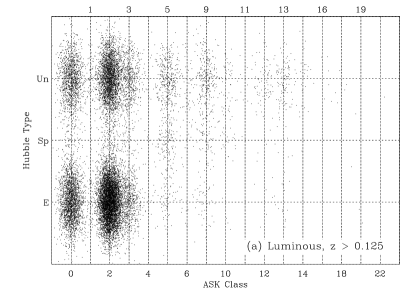
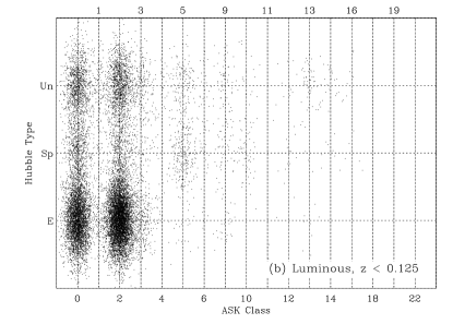
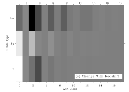
Figure 12.— Variation with redshift of the scatter plot Hubble type vs ASK class. A volume limited sample of luminous Galaxy Zoo targets ($M_{g}<-22.3$) has been divided in two redshift bins – (a) from 0.125 to 0.25, and (b) from 0 to 0.125. (c) Image with the difference between the distributions of galaxies shown at (a) and (b) – white corresponds to a growth towards low redshift. Note the increase of Sps of all ASK classes at low redshift, partly at the expense of unclassified objects (Un). However, the augment of red ASK 0 galaxies cannot be explained as a leakage of Un objects. We interpret it as the aging of the stellar populations. Panels (a) and (b) contain the same number of points, and the image in (c) has been scaled between minimum and maximum.

The morphological classification used for reference only includes redshifts smaller than 0.1 (§ 3.1). One needs a time baseline as long as possible to investigate changes with redshift, therefore, we decided to use the complete sample containing galaxies up to redshift $0.25$, corresponding to a lookback time of the order of 3.5 Gyr. This time is long enough for the galaxies to undergo significant changes in both the morphological structures and the colors – arms do not persist longer than a few Gyrs if the gas that feeds on-going star formation is removed (e.g., Bekki et al. 2002), and blue galaxies become red in much less than a Gyr if star formation shuts off (e.g., Blanton 2006). Consequently, the temporal baseline of the analyzed SDSS/DR7 catalog is long enough to see the scatter plot evolving between redshift $0.25$ and the present. Do we see it? Figures 12a and 12b show scatter plots of a volume limited subsample of the Galaxy Zoo 1 match presented above (§ 3.5). We have selected all the galaxies bright enough to be part of the SDSS/DR7 spectroscopic sample even if they were at redshift 0.25 (i.e., galaxies with absolute $r$ magnitude smaller than $-22.3$, or with apparent magnitude smaller than the completeness limit of SDSS even at redshift 0.25). The use of a volume limited sample is mandatory since blue ASK classes are systematically less luminous than the red ones and, therefore, they artificially disappear at high redshift from SDSS (see, e.g., Sánchez Almeida et al. 2010). A glance at Figs.  12a and 12b shows how the number of red Sps increases in the low redshift sample at the expense of the Un. The change is even more evident in Fig.  12c, which displays an image with the difference between the histograms at low redshift and at high redshift – white corresponds to an increase at low redshift. A part of this increase seems to be due to the improvement of angular resolution at low redshift. Insufficient resolution leads to small spirals being misclassified as Un, whereas Un tend to be classified as E. The final Galaxy Zoo 1 classification acknowledges this bias, and corrects the classes accordingly (Lintott et al. 2010), but residuals seem to remain after correction. In addition to this increase of Sps, the scatter plots in Figs.  12a and b show an increase of ASK 0 galaxies at low redshift, both of Sp and E galaxies. The increase clearly stands out in Fig.  12c. This augment cannot be explained by the Hubble type misclassification described above, which would not change the galaxy ASK class. Similarly, it cannot be ascribed to aperture effects caused by the red centers of the galaxies contributing more at low redshift, because this effect is expected to be largest in spirals whereas the observed increase mainly affects E. We attribute the systematic reddening of the red galaxies as an aging of their stellar populations. Models for the passive evolution of large ellipticals indicate that their colors redden by $\Delta(g-r)\simeq-0.2$ in 1.5 Gyr (e.g., Maraston et al. 2009), which is equivalent to changing colors from ASK 2 to ASK 0 in the time interval between the two redshift bins (Sánchez Almeida et al. 2010, Table 2).

As far as the few blue luminous galaxies included in Fig. 12, it is not at all clear whether they redden, or if their population remains statistically unchanged at low redshift. Studying the redshift variation of the blue classes requires using the full sample, following an analysis in the vein of that in appendix A. We do not address it here because the bias of the match ASK class vs Galaxy Zoo 1 is not purely Malmquist bias, and computing the volume associated with each galaxy is more complex than just applying equation (A4). The task goes beyond the scope of this work, however, in view of the variations observed in red luminous galaxies, it is an exercise deserving follow up.

6. Discussion and Conclusions

There is a general trend for the local galaxies in red ASK classes to show early morphological types, and for the galaxies in blue ASK classes to have late morphological types (Fig. 1a). However, the relationship has a large scatter with a standard deviation between 2 and 3 types, both for the dispersion of Hubble types given an ASK class, and for the dispersion of spectroscopic classes fixed the Hubble type (Tables 2 and 3, columns labeled $a$). Figure 2 shows galaxy images that illustrate the various parts of the scatter plot – the main trend along the diagonal, as well as the outliers represented by red spirals (upper left) and blue ellipticals (bottom right). The distributions of Hubble types given an ASK class are very skewed; they present long tails that go to the late morphological types for the red galaxies, and to the early morphological types for the blue spectroscopic classes. The scatter is not produced by problems in the classification, and it is not reduced when particular subsets are considered – low and high galaxy masses, low and high density environments, barred and non-barred galaxies, face-on galaxies, small and large galaxies, or when a volume limited sample is considered.

The upper left corner of the scatter plot is truly devoid of targets, i.e., there is a remarkable lack of Sd, Sdm, Im and Sm galaxies with red spectra. These morphological types are associated with low mass galaxies, and we interpret this lack as an indication that, for these particular galaxies, the time scale for the morphological changes is shorter than that for the spectral changes. When these very late type galaxies evolve, their Hubble type must become earlier before they become redder. On the contrary, there are plenty of red Sa – Sc galaxies, suggesting that a galaxy can change spectrum while maintaining a Hubble type, provided the galaxy is massive enough. We have found that 68% of the red galaxies (ASK 0, 2 and 3) in the catalog used for reference (Nair & Abraham 2010) are spirals rather then ellipticals. Even though red spectra are not associated with ellipticals, most ellipticals do have red spectra: 97% of the ellipticals in Nair & Abraham (2010) belong to ASK 0, 2 or 3 whereas only 3% of them are blue.

According to their colors, most local galaxies can be split into red galaxies (red sequence) and blue galaxies (blue cloud; e.g., Strateva et al. 2001; Balogh et al. 2004; Baldry et al. 2004). The color gap is not sharp so that in between the two extremes one finds galaxies with intermediate colors on the so-called green valley. These are thought to be transition galaxies (e.g., Martin et al. 2007; Salim et al. 2007). The ASK classification managed to isolate the green valley into a single class ASK 5 (Sánchez Almeida et al. 2010). We find most of ASK 5 galaxies being spiral (§ 3.1). Since the galaxies in the blue cloud are spiral as well, the green valley galaxies seem to be in transit from the blue cloud to the red sequence, with the transition involving no major morphological change. The existence of red spirals mentioned above means that the red sequence is populated by both spheroids and disks. If the galaxies in the green valley were rejuvenated red galaxies with recent star-formation activity, they should present the mixture of E and Sp types characteristic of the red sequence, which is not observed. The fact that the blue cloud preferentially contains late morphological types but the red sequence is not dominated by early types seems to be well established in the literature (e.g., Deng et al. 2009; Blanton & Moustakas 2009).

We explore the dependence of the scatter plot Hubble type vs ASK class on the environment (§ 3.1). Nair & Abraham (2010) provide a measurement of the local density estimated from the distance to the 4th or 5th nearest neighbor, and we find almost no dependence of the relationship on whether low or high density environment galaxies are selected. Of course early types are more often present in dense environments, but we do not find that the relationship with spectral class tightens or becomes more loose in dense environments (but see the comment on S0s below). This result is consistent with the idea expressed by Blanton & Moustakas (2009) that the environment affects the probability of finding early types or late types, but once a particular galaxy is chosen, its properties depend little on the environment. In this sense, the possibility of presenting varied spectra given the Hubble type seems to be a property of the individual galaxies, rather than being stimulated or directed by nearby galaxies. On top of this overall stability of the relationship, we note a slight excess of S0s with respect to Es in dense environments. This trend seems to agree with the finding that S0s become relatively more frequent towards the centers of the clusters (e.g., Dressler 1980; Aguerri et al. 2004).

We investigate variation with redshift of the color-shape relationship using a volume limited subsample mainly formed by luminous red galaxies (§ 5). From redshift $0.25$ to now some galaxies redden as expected from the passive evolution of their stellar populations.

One of the ASK classes, number 6, is known to gather active galactic nuclei (AGNs, Sánchez Almeida et al. 2010). This class seems to be formed by galaxies with a wide range of Hubble types, from E to Sd – see Fig. 1a as well as Table 2, the later showing this class to have a large negative kurtosis characteristic of a spreadout distribution function. This spread of morphological types is a known property of AGNs (e.g. Gabor et al. 2009; Griffith & Stern 2010, and references therein).

Two of the red ASK classes, 1 and 4, have been found to be dominated by edge-on (dust-reddened) spirals. In an analysis not mentioned in the preceding sections, we reproduced the template spectrum characteristic of ASK 1 and 4 with reddened spectra of bluer ASK classes. One finds a good match of both line and continuum assuming a one magnitude extinction at $H\beta$ distributed according to a Milky Way-like law (Cardelli et al. 1989). The fact that ASK 1 and 4 are edge-on disks makes them suitable for a number of studies – for example, determining of the distribution of disk thicknesses (e.g., Sánchez-Janssen et al. 2010), or studying physical properties of the dust associated with ongoing star formation. They may also be used to calibrate weak lensing reconstructions since we know their intrinsic (highly elongated) shapes given the spectrum (e.g., Zhang 2010, and references therein).

The classification based on galSVM and described in § 3.4 is, in fact, a spectro-morphological classification. It includes colors together with other purely morphological parameters. Surprisingly, the use of color does not reduce the scatter of the relationship between spectroscopic class and morphological type. The result is revealing, reflecting that the scatter of colors given a Hubble type is intrinsic.

The present work quantifies the relationship and scatter between Hubble type and spectroscopic class existing in the local universe. It constrains the models and theories of galaxy evolution which should be able to account, not only for the global trend, but also for the scatter. In other words, the challenge lies in explaining how and why galaxies with the same morphology end up with very different spectra, and how and why galaxies with similar spectra may have different Hubble types.

Appendix A $V_{\rm max}$ approach to transform the magnitude limited sample of Nair & Abraham (2010) to a volume limited sample

Following Sánchez Almeida et al. (2008, § 4), the 2D histogram with the number of galaxies having ASK class $A$ and Hubble type $T$ can be written down as a sum over all the galaxies in the sample,

$$N(A,T)=\sum_{i}\,\Pi\big{(}{{A_{i}-A}\over{\Delta A}}\big{)}\,\Pi\big{(}{{T_{i}-T}\over{\Delta T}}\big{)}.$$ (A1)

As usual, the symbol $\Pi$ stands for the rectangle function,

$$\Pi(x)=\cases{1&$|x|<1/2$,\cr 0&elsewhere,}$$ (A2)

and $\Delta T$ and $\Delta A$ represent the bin sizes of the 2D histogram. Rather than the histogram of observed galaxies, $N(A,T)$, we want the histogram to be obtained if galaxies were drawn from a volume limited sample, ${\Large n}(A,T)$. It can be estimated as

$$n(A,T)=\sum_{i}\,\Pi\big{(}{{A_{i}-A}\over{\Delta A}}\big{)}\,\Pi\big{(}{{T_{i}-T}\over{\Delta T}}\big{)}{1\over{V_{i\,{\rm max}}}}$$ (A3)

where $V_{i\,{\rm max}}$ is the maximum volume at which the galaxy $i$ could have been detected in our observation. $V_{i\,{\rm max}}$ depends on properties of the galaxy $i$, as well as on the biases affecting the observation. Equation (A3) implicitly assumes the volume sampled by the observation to be uniform, with the observational biases to be such that they allow us to detect all types of galaxies. We compute the maximum volume as

$$V_{i\,{\rm max}}={W\over 3}10^{-{3\over{5}}(M_{i}+9)}\,{\rm Mpc}^{3},$$ (A4)

with $M_{i}$ the absolute magnitude of the galaxy, and $W$ the solid angle covered by the survey. The previous expression assumes the observation to be magnitude limited (which is approximately correct for the sample, with a limit magnitude of 16), and neglects the bias associated with the surface brightness threshold (see the references given in Sánchez Almeida et al. 2008).

References

- Aaronson (1978) Aaronson, M. 1978, ApJ, 221, L103
- Abazajian et al. (2009) Abazajian, K. N., Adelman-McCarthy, J. K., Agüeros, M. A., et al. 2009, ApJS, 182, 543
- Abraham et al. (1994) Abraham, R. G., Valdes, F., Yee, H. K. C., & van den Bergh, S. 1994, ApJ, 432, 75
- Aguerri et al. (2004) Aguerri, J. A. L., Iglesias-Paramo, J., Vilchez, J. M., & Muñoz-Tuñón, C. 2004, AJ, 127, 1344
- Aguerri et al. (2009) Aguerri, J. A. L., Méndez-Abreu, J., & Corsini, E. M. 2009, A&A, 495, 491
- Aguerri & Trujillo (2002) Aguerri, J. A. L. & Trujillo, I. 2002, MNRAS, 333, 633
- Ascasibar & Sánchez Almeida (2011) Ascasibar, Y. & Sánchez Almeida, J. 2011, MNRAS, in press, arXiv:1104.1388 [astro-ph.CO]
- Baldry et al. (2004) Baldry, I. K., Glazebrook, K., Brinkmann, J., et al. 2004, ApJ, 600, 681
- Balogh et al. (2004) Balogh, M. L., Baldry, I. K., Nichol, R., et al. 2004, ApJ, 615, L101
- Barazza et al. (2008) Barazza, F. D., Jogee, S., & Marinova, I. 2008, ApJ, 675, 1194
- Bekki et al. (2002) Bekki, K., Couch, W. J., & Shioya, Y. 2002, ApJ, 577, 651
- Bershady (1995) Bershady, M. A. 1995, AJ, 109, 87
- Bishop (2006) Bishop, C. M. 2006, Pattern Recognition and Machine Learning (NY: Springer)
- Blanton (2006) Blanton, M. R. 2006, ApJ, 648, 268
- Blanton et al. (2003) Blanton, M. R., Hogg, D. W., Bahcall, N. A., et al. 2003, ApJ, 594, 186
- Blanton & Moustakas (2009) Blanton, M. R. & Moustakas, J. 2009, ARA&A, 47, 159
- Buta et al. (2010) Buta, R., Laurikainen, E., Salo, H., & Knapen, J. H. 2010, ApJ, 721, 259
- Cardelli et al. (1989) Cardelli, J. A., Clayton, G. C., & Mathis, J. S. 1989, ApJ, 345, 245
- Connolly et al. (1995) Connolly, A. J., Szalay, A. S., Bershady, M. A., Kinney, A. L., & Calzetti, D. 1995, AJ, 110, 1071
- Conselice (2006) Conselice, C. J. 2006, MNRAS, 373, 1389
- de la Calleja & Fuentes (2004) de la Calleja, J. & Fuentes, O. 2004, MNRAS, 349, 87
- de Vaucouleurs (1994) de Vaucouleurs, G. 1994, presented at Quantifying Galaxy Morphology at High Redshift, a workshop held at the Space Telescope Science Institute, Baltimore MD, April 27-29 1994