Abstract

Recently Verlinde proposed that gravity can be described as an emergent phenomena arising from changes in the information associated with the positions of material bodies. By using noncommutative geometry as a way to describe the microscopic, microstructure of quantum spacetime, we derive modified Friedmann equation in this setup and study the entropic force modifications to the inflationary dynamics of early universe.
PACS: 02.40.Gh,  11.10.Nx,  04.50.-h,  98.80.Cq
Key Words: Entropic Force, Inflation, Spacetime Noncommutativity

1 Introduction

Recently, Verlinde [1] proposed an idea similar to Jacobson s thermodynamic derivation of the Einstein equations [2], where it is argued that Newton’s law of gravitation can be understood as an entropic force caused by information changes when a material body moves away from the holographic screen. There are some interesting consequences arising from this argument. One is that with the assumption of the entropic force together with the Unruh temperature [3], Verlinde is able to derive the second law of Newton. The other is that the assumption of the entropic force together with the holographic principle and the equipartition law of energy leads to Newton’s law of gravitation. Consequences of Verlinde’s proposal in cosmology have been widely studied [4,5,6]. The inflationary dynamics of a universe governed by entropic gravity also has been studied [7].

To derive the Newton’s law from thermodynamics, Verlinde considered a system consisting of two masses, one test mass $m$ and a source mass $M$. One can consider a surface $\Omega$ centered around $M$ and lying between the two masses. One also assumes $m$ to be at a distance from $\Omega$ smaller with respect to its reduced Compton wavelength $\lambda_{m}=\hbar/(mc)$. Verlinde then proposed that when the test particle moves in the vicinity of the holographic screen $\Omega$, the change in entropy is proportional to the displacement $\Delta x$ i.e.

$$\Delta S_{\Omega}=2\pi k_{B}\frac{\Delta x}{\lambda_{m}}\,.$$ (1)

Number of bits of information stored in the surface of $\Omega$ is given by

$$N=\frac{A_{\Omega}}{l^{2}_{p}}$$ (2)

where $l_{p}$ is the Planck length. The surface of $\Omega$ is in thermal equilibrium at the temperature $T$, all bites are equally likely and the energy of $\Omega$ is equipartitioned among them i.e.

$$U_{\Omega}=\frac{1}{2}Nk_{b}T$$ (3)

where $U_{\Omega}$  is equal to the rest mass of the source $Mc^{2}$. From thermodynamical equation of this system, a force $F$ will arise

$$F\Delta x=T\Delta S_{\Omega}\,.$$ (4)

From the above argument, one can reach the gravitational law of Newton i.e $F=GMm/r^{2}$, (see [1] for more details).

2 Noncommutative geometry inspired entropic correction to Newton’s law

To link this entropic interpretation of gravity with noncommutative geometry, one should consider entropy as a tool to connect the standard description of gravity with the underlying microstructure of a quantum spacetime. Here we use noncommutative geometry to describe the microscopic structure of spacetime manifold. Inspired by some aspects of string theory and loop quantum gravity, the basic idea of noncommutative geometry is that due to existence of a fundamental minimal length (Planck or string length), the coordinate operators also fail to commute. In this case, the fuzziness of spacetime can be expressed using the following relation for non-commutativity of coordinate operators [8,9]

$$[\hat{x}^{i},\hat{x}^{j}]=i\theta^{ij}$$ (5)

where $\theta^{ij}$ is a real, antisymmetric matrix, with the dimension of length squared which determines the fundamental cell discretization of spacetime manifold. As a consequence of above relation, the notion of point in the spacetime manifold becomes obscure as there is a fundamental uncertainty in measuring the coordinates

$$\Delta x^{i}\Delta x^{j}\geq\frac{1}{2}|\theta^{ij}|.$$ (6)

The presence of noncommutativity enforces some modifications on Verlinde assumptions [10]. First due to uncertainty on the surface $\Omega$, there exists a fundamental unit for entropy change, $\Delta S_{\theta}$ which is realized at the displacement $\Delta x_{min}$. Therefore the change of entropy is

$$\Delta S_{\Omega}=\Delta S_{\theta}(\frac{\Delta x}{\Delta x_{min}})\,.$$ (7)

This equation states that when the test mass $m$ is a distance $\Delta x_{min}$ away from the surface, the entropy of the surface changes by one fundamental unit $\Delta S_{\theta}$. In other words, due to existence of a minimal length, $\Delta x_{min}$, there is a minimum change of entropy as $\Delta S_{\theta}$. A general displacement $\Delta x$ then results in a change in entropy as equation (7), where $(\frac{\Delta x}{\Delta x_{min}})$ is an integer number.

Secondly, on the surface $\Omega$ the unit surface is $\theta$. So the number of information bits is

$$N=\frac{A_{\Omega}}{\theta}\,.$$ (8)

Using these assumptions, the entropic modification to Newton’s law has been derived in [10] as

$$F=\frac{Mm}{r^{2}}\Big{(}\frac{4c^{3}\theta^{2}}{\hbar\alpha^{2}}\Big{)}\bigg{[}\frac{c^{3}}{4\hbar G}+\frac{\partial s}{\partial A}\bigg{]}$$ (9)

where $\alpha$ is defined as

$$\alpha=\frac{8\pi\Delta x_{min}}{\lambda_{m}}\,.$$ (10)

For the entropic force in (9) to coincide with the Newton’s law, we should set the noncommutative parameter $\theta$ as $\theta=\alpha l^{2}_{p}$. Doing this, the modified Newton’s law reads

$$F=\frac{GMm}{r^{2}}\bigg{[}1+4l^{2}_{p}\frac{\partial s}{\partial A}\bigg{]}\,,$$ (11)

which coincides with the Newton’s law to the first order. One should note that the second term in the bracket is a quantum correction which arises when one considers quantum gravity corrections to the entropy-area relation [11]. If we neglect the quantum effects, the second term in (11) vanishes.

With the same assumptions, the temperature of the noncommutative holographic screen will be [10]

$$T=\frac{M}{r^{2}}\frac{\theta c^{2}}{2\pi k_{B}}\,.$$ (12)

From this equation, it is obvious that a noncommutative manifold is equivalent to a thermodynamical system whose temperature is given by the above relation.

To obtain the explicit modification of Newton’s law caused by entropic corrections, we should have the specific entropy-area relation in eq. (11). To achieve this goal, we use the coherent state picture of noncommutativity first proposed in Ref. [12] as our underlying microstructure of a quantum spacetime. This approach eliminates point-like structures in the favor of smeared objects. Using this approach for obtaining the entropy/area relation with the help of black hole thermodynamics, the modified Newton’s law has been derived in Ref. [10] as

$$F=\frac{GMm}{r^{2}}\bigg{[}1+\frac{\Gamma(3/2;(r^{2}/4\pi\theta))}{\gamma(3/2;(r^{2}/4\pi\theta))}\bigg{]}$$ (13)

where $\Gamma(3/2;(r^{2}/4\pi\theta))$ and $\gamma(3/2;(r^{2}/4\pi\theta))$ are incomplete upper and lower gamma functions respectively. In the low energy or large distance limit( $r\gg\theta$ ), this reduces to

$$F\simeq\frac{GMm}{r^{2}}\bigg{[}1+\frac{re^{-r^{2}/(4\alpha l^{2}_{p})}}{\sqrt{\pi\alpha}l_{p}}+\frac{r^{2}e^{-r^{2}/(2\alpha l^{2}_{p})}}{2\alpha\sqrt{\pi}l^{2}_{p}}\bigg{]}\,.$$ (14)

In the next section we will use this modified force to obtain the cosmological dynamics of the universe using the approach of Newtonian cosmology.

3 Cosmological dynamics

To obtain cosmological dynamics in this scenario, we assume that the background spacetime is spatially homogeneous and isotropic and is given by the Friedmann-Robertson-Walker (FRW) metric

$$ds^{2}=h_{ij}dx^{i}dx^{j}+R^{2}\bigg{(}d\vartheta^{2}+\sin^{2}(\vartheta)d\varphi^{2}\bigg{)}\,,$$ (15)

where $i,\,j=0,\,1$. We consider a region of spacetime with volume $V$ with a compact boundary surface $S$. The region is a sphere with radius $R=a(t)r$ where $r$ will remain constant during expansion. Because of the spherical symmetry, this boundary is an equipotential surface such that we may treat it as a holographic screen. Now we assume that in the Newtonian cosmology the background spacetime is Minkowskian. For this region the apparent (Hubble) horizon will be at $R=1/H$. So, we assume that in this setup the holographic screen is at the apparent horizon $R=1/H$ for a flat spacetime. A similar approach could be found in references [4,5,13]. Based on this argument, the dynamical apparent horizon, a marginally trapped surface with vanishing expansion, is given in a FRW background by

$$R=ar=\frac{1}{\sqrt{H^{2}+k/a^{2}}}\,.$$ (16)

We assume also that matter source in the FRW universe is a perfect fluid with stress-energy tensor

$$T_{\mu\nu}=(\rho+p)u_{\mu}u_{\nu}+pg_{\mu\nu}\,.$$ (17)

The system also obeys the usual continuity equation as

$$\dot{\rho}+3H(\rho+p)=0\,.$$ (18)

With these assumptions and using the modified force (14), now we find the acceleration equation following the procedures of Newtonian cosmology. We consider a region of spacetime with volume $V$ with a compact surface $S$. The region is a sphere with radius $R=a(t)r$ where $r$ remains constant during expansion. Applying Newton’s second law and using the force as given in (14) for a test mass near the surface $S$, we get

$$F=ma=m\ddot{R}=mr\ddot{a}=-\frac{GMm}{r^{2}}\bigg{[}1+\frac{re^{-r^{2}/(4\alpha l^{2}_{p})}}{\sqrt{\pi\alpha}l_{p}}+\frac{r^{2}e^{-r^{2}/(2\alpha l^{2}_{p})}}{2\alpha\sqrt{\pi}l^{2}_{p}}\bigg{]}\,.$$ (19)

Given that $\rho=M/V$ and $V=\frac{4}{3}\pi a^{3}r^{3}$, equation (19) can be rewritten as

$$\frac{\ddot{a}}{a}=-\frac{4\pi G}{3}\rho\bigg{[}1+\frac{Re^{-R^{2}/(4\alpha l^{2}_{p})}}{\sqrt{\pi\alpha}l_{p}}+\frac{R^{2}e^{-R^{2}/(2\alpha l^{2}_{p})}}{2\alpha\sqrt{\pi}l^{2}_{p}}\bigg{]}\,.$$ (20)

To obtain the correct Friedmann equation of the model, we note that it is the active gravitational mass ${\cal{M}}$ in the spatial region $V$ rather than the total mass $M$ that produces the acceleration [4]. The active gravitational mass or Tolman-Komar mass [14], is defined as

$${\cal{M}}=2\int dV(T_{ab}-\frac{1}{2}Tg_{ab})u^{a}u^{b}=(\rho+3p)\frac{4}{3}\pi a^{3}r^{3}$$ (21)

Replacing $M$ with ${cal{M}}$ in (19) we get

$$\frac{\ddot{a}}{a}=-\frac{4\pi G}{3}(\rho+3p)\bigg{[}1+\frac{Re^{-R^{2}/(4\alpha l^{2}_{p})}}{\sqrt{\pi\alpha}l_{p}}+\frac{R^{2}e^{-R^{2}/(2\alpha l^{2}_{p})}}{2\alpha\sqrt{\pi}l^{2}_{p}}\bigg{]}\,.$$ (22)

Using the above acceleration equation and the continuity equation (18), we find the Friedmann equation as follows

$$H^{2}+\frac{k}{a^{2}}=\frac{8\pi G}{3}\rho\bigg{[}1+\frac{Re^{-R^{2}/(4\alpha l^{2}_{p})}}{\sqrt{\pi\alpha}l_{p}}\int\frac{d(\rho a^{2})}{a^{2}}+\frac{R^{2}e^{-R^{2}/(2\alpha l^{2}_{p})}}{2\alpha\sqrt{\pi}l^{2}_{p}}\int\frac{d(\rho a^{2})}{a^{4}}\bigg{]}\,.$$ (23)

If we assume a constant equation of state parameter, then the energy density will be given by $\rho=\rho_{p}a^{-3(1+\omega)}$ where $\rho_{p}$ is an integration constant corresponding to present value of the energy density. In this case the integrals in Friedmann equation (23) can be solved analytically to find

$${H}^{2}+{\frac{k}{{a}^{2}}}=\frac{8\pi\,G}{3}\rho\Bigg{[}1+\frac{(1+3\,\omega)}{3(1+\omega)\sqrt{\pi\,\theta}}\rm R{{\rm e}^{-{\frac{{R}^{2}}{4\theta}}}}+\frac{(1+3\,\omega)}{(5+3\omega)\sqrt{\pi}\theta}\rm R^{2}{{\rm e}^{-{\frac{{R}^{2}}{2\theta}}}}\Bigg{]}\,.$$ (24)

The existence of exponential terms in the acceleration equation has interesting consequences at very early times in the inflation era. First of all, it should be noted that the terms in the brackets of equation (24) ( and similarly in equation (22)) are positive for ordinary matter fields, so we still need $\rho+3p<0$ to have inflation. Fortunately, noncommutativity provides the negative pressure needed for a successful inflation. To examine this, we use a newly proposed model for noncommutative inflation introduced in [15]. The basic idea is that the initial singularity is smeared due to spacetime noncommutativity. One could split the energy density on any hypersurface as [15]

$$\rho=\rho_{0}e^{-|T|^{2}/4\theta}e^{-|\vec{{X}}|^{2}/4\theta}$$ (25)

where $R^{2}=T^{2}+|\vec{X}|^{2}$ and $T=it$ is the Euclidean time. From one hypersurface to another, the $\vec{X}$-dependent part of $\rho$ does not change, so it can be included into $\rho_{0}$. Therefore, one could write the energy density of the smeared initial singularity as [10]

$$\rho(t)=\rho_{0}\,e^{-t^{2}/4\theta}\,.$$ (26)

Using equation (16) for apparent horizon $R$, the Friedmann equation (22) could be solved analytically to obtain the scale factor $a(t)$ as

$$a(t)\simeq\exp\bigg{[}\frac{4}{3}\pi\,\sqrt{3G{\rho_{0}}\,\theta}\,\,{{\rm erf}({\frac{t}{2\sqrt{2\theta}}})}\bigg{]}$$

$$+{\frac{{{\rm e}^{{\frac{t}{2\sqrt{2\theta}}}}}}{256\sqrt{\pi}\theta^{2}}}\,\bigg{[}\frac{\sqrt{2\pi}}{8}{t}^{5}{{\rm e}^{{\frac{t}{2\sqrt{2\theta}}}}}{\theta}^{-5/2}+{\frac{25}{64}}\,{\rm Ei}(1,\,{\frac{t}{2\sqrt{2\theta}}}){t}^{4}{{\rm e}^{{\frac{t}{2\sqrt{2\theta}}}}}{\theta}^{-2}+{\frac{7}{8}}\,{\frac{{t}^{2}}{\theta}}+{\frac{7\sqrt{2}}{32}}\,{\frac{{t}^{3}}{{\theta}^{3/2}}}+{\frac{t\sqrt{2}}{2\sqrt{\theta}}}+6\bigg{]}\,,$$ (27)

where ${\rm\,Ei}(a,z)$ is the exponential integral defined as ${\rm\,Ei}(a,z)=z^{a-1}\Gamma(1-a,z)$.

Using the continuity equation (18), pressure is given by

$$p={\rho_{0}}\,{{\rm e}^{-{\frac{{t}^{2}}{4\theta}}}}\Bigg{\{}16384\,\sqrt{\pi}t{\theta}^{5}\exp\Bigg{[}{\frac{4\sqrt{3}}{3}\pi\,\sqrt{G{\rho_{0}}\,\theta}\,\,{{\rm erf}({\frac{t}{2\sqrt{2\theta}}})}}\Bigg{]}+{{\rm e}^{{\frac{t}{\sqrt{2\theta}}}}}\Bigg{[}8\,\sqrt{\pi}{t}^{6}\sqrt{2\theta}+25\,{t}^{5}\theta\,{\rm Ei}(1,{\frac{t}{2\sqrt{2\theta}}})\Bigg{]}$$

$$+{{\rm e}^{{\frac{t}{2\sqrt{2\theta}}}}}\Bigg{[}164\,{t}^{3}{\theta}^{2}+14\,{t}^{4}{\theta}^{3/2}\sqrt{2}-384\,{\theta}^{3}t-304\,\sqrt{2}{t}^{2}{\theta}^{5/2}\Bigg{]}$$

$$-65536\,\pi\,\sqrt{3}\sqrt{G{\rho_{0}}\,\theta}{\theta}^{11/2}\exp\Big{[}\frac{1}{24}(-3{t}^{2}+32\pi\,\sqrt{6}\sqrt{G{\rho_{0}}\,\theta}\,\,{{\rm erf}(\frac{t}{2\sqrt{2\theta}})}\Big{]}-{{\rm e}^{{\frac{t}{\sqrt{2\theta}}}}}\Bigg{[}240\sqrt{2\pi}\,{\theta}^{3/2}{t}^{4}$$

$$-48\theta\,{t}^{5}\sqrt{\pi}-600{\theta}^{2}{\rm Ei}(1,{\frac{t}{2\sqrt{2\theta}}}){t}^{3}-75\,\sqrt{2}{t}^{4}{\theta}^{3/2}{\rm Ei}(1,{\frac{t}{2\sqrt{2\theta}}})\Bigg{]}$$

$$-768\,{{\rm e}^{{\frac{t}{2\sqrt{2\theta}}}}}{\theta}^{7/2}\sqrt{2}\Bigg{\}}\times{\theta}^{-1}\times\Bigg{\{}65536\,\pi\,\sqrt{3G{\rho_{0}}\,\theta}\exp\Big{[}{\frac{1}{24}(-3\,{t}^{2}+32\,\pi\,\sqrt{3}\sqrt{G{\rho_{0}}\,\theta}\,\,{{\rm erf}({\frac{t}{2\sqrt{2\theta}}})})}\Big{]}\sqrt{2}{\theta}^{9/2}$$

$$+{{\rm e}^{{\frac{t}{\sqrt{2\theta}}}}}\Bigg{[}240\,\sqrt{2\pi\theta}{t}^{4}+48\,{t}^{5}\sqrt{\pi}+600\,\theta\,{\rm Ei}(1,{\frac{t}{2\sqrt{2\theta}}}){t}^{3}+75\,\sqrt{\theta}{\rm Ei}(1,{\frac{t}{2\sqrt{2\theta}}}){t}^{4}\sqrt{2}\Bigg{]}$$

$$-{{\rm e}^{{\frac{t}{2\sqrt{2\theta}}}}}\Bigg{[}108\,{t}^{3}\theta\,+768\,{\theta}^{2}t+336\,\sqrt{2}{t}^{2}{\theta}^{3/2}+768\,\sqrt{2}{\theta}^{5/2}\Bigg{]}\Bigg{\}}^{-1}\,.$$ (28)

And the equation of state parameter will be

$$\omega=-\Bigg{\{}-16384\,\sqrt{\pi}t{\theta}^{5}\exp\Big{[}{\frac{4}{3}\pi\,\sqrt{3G{\rho_{0}}\,\theta}\,\,{{\rm erf}({\frac{t}{2\sqrt{2\theta}}})}}\Big{]}-8\,{t}^{6}\sqrt{\theta}\sqrt{2}{{\rm e}^{1/2\,{\frac{t\sqrt{2}}{\sqrt{\theta}}}}}\sqrt{\pi}-25\,{t}^{5}\theta\,{\rm Ei}(1,{\frac{t}{2\sqrt{2\theta}}}){{\rm e}^{{\frac{t}{\sqrt{2\theta}}}}}$$

$$-{{\rm e}^{{\frac{t}{2\sqrt{2\theta}}}}}\Bigg{[}164\,{t}^{3}{\theta}^{2}-14\,\sqrt{2}{t}^{4}{\theta}^{3/2}+384\,{\theta}^{3}t+304\,\sqrt{2}{t}^{2}{\theta}^{5/2}\Bigg{]}$$

$$+65536\,\sqrt{2}\pi{\theta}^{11/2}\,\sqrt{3G{\rho_{0}}\,\theta}\exp\Big{[}{\frac{1}{24}(-3\,{t}^{2}+32\,\pi\,\sqrt{3G{\rho_{0}}\,\theta}\,\,{{\rm erf}({\frac{t}{2\sqrt{2\theta}}})})}\Big{]}$$

$$+{{\rm e}^{{\frac{t}{\sqrt{2\theta}}}}}\Bigg{[}240\,{\theta}^{3/2}{t}^{4}\sqrt{2\pi}+48\,\theta\,{t}^{5}\sqrt{\pi}+600\,{\theta}^{2}{\rm Ei}(1,{\frac{t\sqrt{2}}{4\sqrt{\theta}}}){t}^{3}+75\,\sqrt{2}{\theta}^{3/2}{\rm Ei}(1,{\frac{t}{2\sqrt{2\theta}}}){t}^{4}\Bigg{]}$$

$$+768\,\sqrt{2}{{\rm e}^{{\frac{t}{2\sqrt{2\theta}}}}}{\theta}^{7/2}\Bigg{\}}\times{\theta}^{-1}\times\Bigg{\{}65536\,\pi\,\sqrt{3G{\rho_{0}}\,\theta}\exp\Big{[}{\frac{1}{24}(-3\,{t}^{2}+32\,\pi\,\sqrt{3G{\rho_{0}}\,\theta}\,\,{{\rm erf}({\frac{t}{2\sqrt{2\theta}}})})}\Big{]}\sqrt{2}{\theta}^{9/2}$$

$$+{{\rm e}^{{\frac{t}{\sqrt{2\theta}}}}}\Bigg{[}240\,\sqrt{2\pi\theta}{t}^{4}+48\,{t}^{5}\sqrt{\pi}+600\,\theta\,{\rm Ei}(1,{\frac{t}{2\sqrt{2\theta}}}){t}^{3}+75\,\sqrt{2}\sqrt{\theta}{\rm Ei}(1,{\frac{t}{2\sqrt{2\theta}}}){t}^{4}\Bigg{]}$$

$$-{{\rm e}^{{\frac{t\sqrt{2}}{4\sqrt{\theta}}}}}\Bigg{[}108\,{t}^{3}\theta\,+768\,{\theta}^{2}t+336\,\sqrt{2}{t}^{2}{\theta}^{3/2}+768\,\sqrt{2}{\theta}^{5/2}\Bigg{]}\Bigg{\}}^{-1}\,\,.$$ (29)

Although these equations have very complicated form, the physical implications of them are very simple. In figure 1 we show variation of pressure and the equation of state parameter with the cosmic time in the early stages of the universe evolution. The pressure is negative which provides the condition for a successful inflation. Also the plot of equation of state parameter versus the cosmic time shows an accelerating behavior ( $\omega<-\frac{1}{3}$) in early stage of the universe evolution.

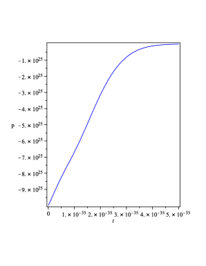
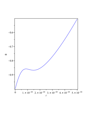
Figure 1: a) Evolution of pressure in a noncommutative spacetime with entropic gravity. The pressure is negative which provides the condition for a successful inflation. b) Evolution of the equation of state parameter in a noncommutative spacetime with entropic gravity. Evidently, this model gives an accelerating behavior ( $\omega<-\frac{1}{3}$) in early stage of the universe evolution.

4 Perturbations

The perturbed flat FRW metric in the longitudinal gauge has the form

$$ds^{2}=-(1+2\Phi)dt^{2}+a^{2}(1-2\Psi)\gamma_{lm}dx^{l}dx^{m}\,$$ (30)

where $\gamma_{lm}$ is the Euclidian metric and $l\,,\,m=1,2,3$. Generally, the perturbations are described by $\Phi$ (the Bardeen potential) and $\Psi$, which both are functions of space and time. Nevertheless, in the absence of noncommutative stress one could set $\Phi=\Psi$. The perturbed Einstein equations are

$$3H(H\Phi+\dot{\Psi})-\frac{1}{a^{2}}\nabla^{2}\Psi=-4\pi G\,\delta\rho$$ (31)

$$H\Phi+\dot{\Psi}=-4\pi G\,\delta q$$ (32)

$$\ddot{\Psi}+3H\dot{\Psi}+H\dot{\Phi}+(2\dot{H}+3H^{2})\Phi-\frac{1}{3a^{2}}\nabla^{2}(\Psi-\Phi)=4\pi Gc^{2}_{s}\,\delta\rho$$ (33)

where $\delta T_{0}^{0}=-\delta\rho$, $\delta T_{i}^{0}=\delta q_{i}$ , $\delta T_{j}^{i}=c^{2}_{s}\delta\rho\delta_{j}^{i}$ and $c_{s}$ is the speed of sound given by $c^{2}_{s}=\frac{\dot{p}}{\dot{\rho}}$ . Vanishing of the anisotropic stress means that we can set $\Phi=\Psi$ in which case. Then, equations (31) and (33) could be combined to give a single equation for the evolution of metric potential $\Phi$ in the momentum space

$$\ddot{\Phi}_{k}+(4+3c^{2}_{s})H\dot{\Phi_{k}}+\Bigg{(}\frac{k^{2}c^{2}_{s}}{a^{2}}+2\dot{H}+3H^{2}(1+c^{2}_{s})\Bigg{)}\Phi_{k}=0\,.$$ (34)

Using the metric potential $\Phi$ , the power spectrum at the time of Hubble crossing , $k=aH$ then is given by

$$P_{\Phi_{k}}=\frac{k^{3}}{2\pi^{2}}\langle\Phi^{2}_{k}\rangle\,.$$ (35)

The curvature perturbation on slices of uniform energy density, $\zeta$, can be calculated from $\Phi$ using the relation

$$\zeta\equiv\Phi-\frac{H}{\dot{H}}(\dot{\Phi}+H\Phi)\,.$$ (36)

Using equation (26), the explicit form of the Hubble parameter in this model is

$$H=\frac{1}{6}\,\Bigg{\{}65536\,\pi\,\sqrt{3G\rho_{0}\,\theta}\exp\Big{[}\frac{1}{24}(-3\,{t}^{2}+32\,\pi\,\sqrt{3}\sqrt{G\rho_{0}\,\theta}){\rm erf}({\frac{t}{2\sqrt{2\theta}}})\Big{]}\sqrt{2}{\theta}^{9/2}$$

$$+\rm e^{{\frac{t}{\sqrt{2\theta}}}}\Bigg{[}240\sqrt{2\pi}\,\sqrt{\theta}{t}^{4}+48\,{t}^{5}\sqrt{\pi}+600\,\theta\,{\rm Ei}(1,{\frac{t}{2\sqrt{2\theta}}}){t}^{3}+75\,\sqrt{2\theta}{t}^{4}{\rm Ei}(1,{\frac{t}{2\sqrt{2\theta}}})\Bigg{]}$$

$$-{{\rm e}^{{\frac{t}{2\sqrt{2\theta}}}}}\Bigg{[}108\,\theta\,{t}^{3}+768\,{\theta}^{2}t+336\,{\theta}^{3/2}{t}^{2}\sqrt{2}+768\,{\theta}^{5/2}\sqrt{2}\Bigg{]}\Bigg{\}}$$

$$\times{\frac{1}{\sqrt{\theta}}}\Bigg{\{}16384\,{\theta}^{9/2}\sqrt{\pi}\exp\Big{(}{\frac{4\sqrt{3}}{3}\pi\,\sqrt{G\rho_{0}\,\theta}{{\rm erf}({\frac{t}{2\sqrt{2\theta}}})}}\Big{)}+8{t}^{5}\sqrt{2}{{\rm e}^{{\frac{t}{\sqrt{2\theta}}}}}\sqrt{\pi}+25\,{\rm Ei}(1,{\frac{t\sqrt{2}}{2\sqrt{2\theta}}}){t}^{4}{{\rm e}^{{\frac{t}{2\sqrt{\theta}}}}}\sqrt{\theta}$$

$$+{{\rm e}^{{\frac{t}{2\sqrt{2\theta}}}}}\Bigg{[}56\,{t}^{2}{\theta}^{3/2}+14\,{t}^{3}\sqrt{2}\theta+384\,{\theta}^{5/2}+32\,t\sqrt{2}{\theta}^{2}\Bigg{]}\Bigg{\}}^{-1}\,.$$ (37)

Given the extremely complicated form of the Hubble parameter and the speed of sound, equation (34) cannot be solved analytically. Instead, we have done a numerical analysis and plotted the evolution of the metric potential $\Phi$ and curvature perturbation. To doing so, we have used the values $\theta=10^{-40}cm$ and $\rho_{0}=10^{26}$. Figures 2 and 3 are results of our numerical analysis. The crucial test for any inflationary model is their ability to produce almost scale invariant spectrum of scalar perturbations. As it has been shown previously [16], noncommutativity generates a small deviation from scale invariance in inflationary scenarios. Also it is expected that nongaussianity should be greater in these models than the usual inflaton field models [17]. To be a realistic model of the early universe and also to test whether or not our model is consistent with recent observational data, we define the slow-roll parameters as usual

$$\epsilon\equiv-\frac{\dot{H}}{H^{2}}$$

$$\eta\equiv\frac{\dot{\epsilon}}{H\epsilon}\,\,.$$ (38)

We assume also that as usual the scalar spectral index is given by the following relation

$$n_{s}-1\simeq-6\epsilon+2\eta.$$ (39)

Evolution of the slow roll parameters $\epsilon$ and $\eta$ versus the cosmic time are given in figure 2 (left panel). Both parameters are small at the time of inflation, leading to an almost scale invariant, slightly red tilted spectrum as depicted in the right panel of this figure. Also figure 3 gives evolution of the metric potential $\Phi$ (dashed line) and curvature perturbation $\zeta$ ( solid line) versus the cosmic time. $\zeta$ is almost constant at the end of inflation while $\Phi$ approaches order of unity at that time. We note that our adopted value of $\rho_{0}=10^{26}$ is chosen so that a sufficient number of e-foldings to solve standard model problems is guaranteed.

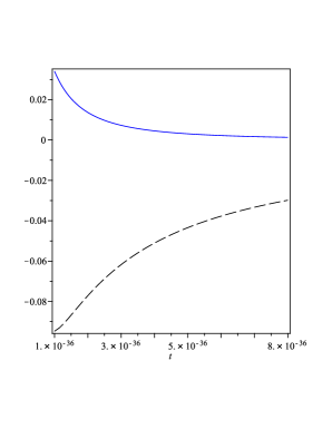
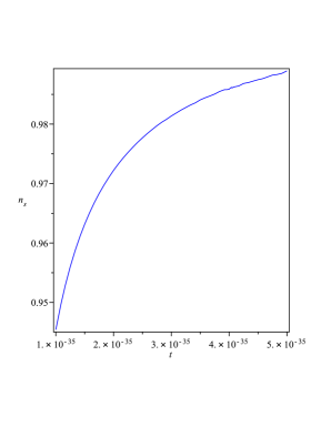
Figure 2: a) Evolution of the slow roll parameters $\epsilon$ (solid line) and $\eta$ (dashed line) versus the cosmic time. Both parameters are small at the time of inflation leading to an almost scale invariant spectrum. b) Evolution of the scalar spectral index versus the cosmic time. Due to value and sign of slow roll parameters, $n_{s}$ derives towards unity at the end of inflation and is slightly red tilted.

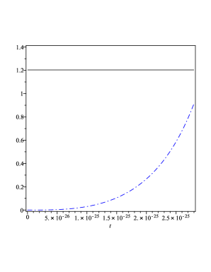
Figure 3: Evolution of the metric potential $\Phi$ (dashed line) and curvature perturbation $\zeta$ (solid line) versus the cosmic time. $\zeta$ is almost constant at the end of inflation while $\Phi$ approaches order of unity at that time.

5 Conclusion

The relation between spacetime noncommutativity and thermodynamics has been known previously and specifically blackhole thermodynamics in noncommutative spaces has been studied extensively [18]. Noncommutativity encodes microscopic degrees of freedom of the quantum spacetime and in this sense, a noncommutative manifold will be equivalent to a thermodynamical system with a temperature given by noncommutative parameter $\theta$. Considering these facts, it seems that there is a deep connection between noncommutativity and thermodynamical description of gravity proposed by Verlinde. Furthermore, both these theories rely on the existence of a fundamental unit of length (Planck or string length) and are similar in this respect too.

Generally it is believed that cosmic microwave background embodies the effects of trans-Planckian physics [19-25]. Noncommutative inflation is a process which imprints these effects to CMB, so there have been various attempts at constructing noncommutative inflationary models to test the results against observations of CMB. One approach is to use relation (5) for space-space coordinates [19,20,26,27] and to construct a noncommutative field theory on the spacetime manifold by replacing ordinary product of fields by Weyl-Wigner-Moyal $\ast$-product. Another approach is to incorporate the fundamental noncommutativity of spacetime into inflationary models via a generalized uncertainty principle (GUP)[28] (see also [16]). Coherent state picture of noncommutativity also has been used to construct inflationary models in both 4D and extra-dimensional scenarios [15, 29].

In this paper we used the coherent state picture of noncommutativity to determine the explicit entropy-area relation in order to determine modified Friedmann equation in a universe governed by entropic gravity. In this setup, negative pressure of noncommutative energy density in very early universe derives it toward an inflationary era. The dynamics of this inflationary epoch and generation of scale invariant scalar perturbations have been studied. In this model, the slow-roll parameters are small at the time of inflation, leading to an almost scale invariant, slightly red tilted spectrum.

Acknowledgment
This work has been supported partially by Research Institute for Astronomy and Astrophysics of Maragha, IRAN.

References

- [1] E. P. Verlinde, [arXiv:1001.0785].
- [2] T. Jacobson, Phys. Rev. Lett. 75, 1260 (1995).
- [3] W. G. Unruh, Phys. Rev. D 14, 870 (1976).
- [4] R. G. Cai, L. M. Cao and N. Ohta, Phys. Rev. D 81, 061501 (2010), [arXiv:1001.3470].
- [5] A. Sheykhi, Phys. Rev. D 81, 104011 (2010), [arXiv:1004.0627]
-
[6]
M. Li and Y. Wang, Phys. Lett. B 687, 243 (2010), [arXiv:1001.4466]
S. W. Wei, Y. X. Liu and Y. Q. Wang, [arXiv:1001.5238]
Y. Ling and J. P. Wu, JCAP 1008, 017 (2010), [arXiv:1001.5324]
D. A. Easson, P. H. Frampton and G. F. Smoot, [arXiv:1002.4278]
U. H. Danielsson, [arXiv:1003.0668]
N. Afshordi, [arXiv:1003.4811]
A. Sheykhi, Phys. Rev. D 81, 104011 (2010), [arXiv:1004.0627]
A. Sheykhi and S. H. Hendi, [arXiv:1011.0676]
M. Li and Y. Pang, Phys. Rev. D 82, 027501 (2010), [arXiv:1004.0877]
T. Qiu, [arXiv:1004.1693]
R. Casadio and A. Gruppuso, [arXiv:1005.0790]
H. Wei, [arXiv:1005.1445]
W. Gu, M. Li and R. -X. Miao, [arXiv:1011.3419]
T. S. Koivisto, D. F. Mota and M. Zumalacarregui, [arXiv:1011.2226]
S. H. Hendi and A. Sheykhi, [arXiv:1012.0381]. -
[7]
D. A. Easson, P. H. Frampton and G. F. Smoot, [arXiv:1003.1528]
M. Li and Y. Pang, Phys. Rev. D 82, 027501 (2010), [arXiv:1004.0877]
Y. F. Cai, J. Liu and H. Li, Phys. Lett. B 690, 213 (2010), [arXiv:1003.4526]
Y. F. Cai and E. N. Saridakis, [arXiv:1011.1245]. -
[8]
M. R. Douglas and N. A. Nekrasov, Rev. Mod. Phys. 73
977, (2001)
R. J. Szabo, Phys. Rept. 378, 207 (2003)
N. Seiberg and E. Witten, JHEP 9909, 032 (1999)
A. Connes and M. Marcolli, [arXiv:math.QA/0601054]
A. Connes, J. Math. Phys. 41, 3832 (2000)
A. Konechny and A. Schwarz, Phys. Rept. 360, 353 (2002)
M. Chaichian et al, Eur. Phys. J. C 29, 413 (2003)
A. Micu and M. M. Sheikh-Jabbari, JHEP 0101, 025 (2001)
M. Panero, JHEP 0705, 082 (2007). -
[9]
G. Veneziano, Europhys. Lett. 2, 199 (1986)
D. Amati, M. Ciafaloni and G. Veneziano, Phys. Lett. B 197, 81 (1987)
D. Amati, M. Ciafaloni and G. Veneziano, Int. J. Mod. Phys. A 3, 1615 (1988)
D. Amati, M. Ciafaloni and G. Veneziano, Nucl. Phys. B 347,530 (1990)
D. J. Gross and P. F. Mende, Nucl. Phys. B 303, 407 (1988)
D. Amati, M. Ciafaloni and G. Veneziano, Phys. Lett. B 216, 41 (1989). - [10] P. Nicolini, Phys. Rev. D 82, 044030 (2010), [arXiv:1005.2996].
-
[11]
A. Strominger and C. Vafa, Phys. Lett. B 379, 99 (1996);
E. Halyo, B. Kol, A. Rajaraman and L. Susskind, Phys. Lett. B 401, 15 (1997);
S. N. Solodukhin, Phys. Rev. D 57, 2410 (1998)
L Modesto, Class. Quant. Grav. 23, 5587-5602 (2006) [arXiv:0509078];
L Modesto, [arXiv:0811.2196 [gr-qc]];
J. Zhang,Phys.Lett. B 668 (2008) 353;
R. Banerjee and B. R. Majhi, Phys. Lett. B 662, 62 (2008);
R. Banerjee and B. R. Majhi, JHEP 0806 (2008) 095; -
[12]
A. Smailagic and E. Spallucci, J. Phys. A 37, 1
(2004), [Erratum-ibid: J. Phys. A 37, 7169 (2004)]
A. Smailagic and E. Spallucci, J. Phys. A 36, L467 (2003)
A. Smailagic and E. Spallucci, J. Phys. A 36, L517 (2003). -
[13]
R. Cai, L. Cao, N. Ohta, Phys. Rev. D 81, 084012 (2010) [arXiv:1002.1136];
F. Shu, Y. Gong,[arXiv:1001.3237] - [14] T. Padmanabhan, Class. Quant. Grav. 21, 4485 (2004) [arXiv:gr-qc/0308070]
- [15] M. Rinaldi, [arXiv:0908.1949].
-
[16]
K. Nozari and S. Akhshabi, Int. J. Mod. Phys. D 19, 513
(2010), [arXiv:0910.2808]
Q. G. Huang, M. Li, Nucl. Phys. B 713, 219 (2005)
Q. G. Huang, M. Li, Nucl. Phys. B 755, 286 (2006)
S. Koh, R.H. Brandenberger, JCAP 0706, 021 (2007). - [17] K. Fang, B. Chen and W. Xue, Phys. Rev. D77, 063523 (2008).
-
[18]
P. Nicolini, A. Smailagic and E. Spallucci, ESA Spec. Publ.
637, 11.1 (2006), [arXiv:hep-th/0507226]
P. Nicolini, J. Phys. A 38, L631 (2005), [arXiv:hep-th/0507266]
P. Nicolini, A. Smailagic and E. Spallucci, Phys. Lett. B 632, 547 (2006), [arXiv:gr-qc/0510112]
S. Ansoldi, P. Nicolini, A. Smailagic and E. Spallucci, Phys. Lett. B 645, 261 (2007), [arXiv:gr-qc/0612035]
E. Spallucci, A. Smailagic and P. Nicolini, Phys. Lett. B 670, 449 (2009), [arXiv:0801.3519]
Y. S. Myung and M. Yoon, Eur. Phys. J. C 62, 405 (2009), [arXiv:0810.0078]
M. I. Park, Phys. Rev. D 80, 084026 (2009), [arXiv:0811.2685]
R. Garattini and F. S. N. Lobo, Phys. Lett. B 671, 146 (2009), [arXiv:0811.0919]
P. Nicolini and E. Spallucci, Class. Quant. Grav. 27, 015010 (2010), [arXiv:0902.4654]
I. Arraut, D. Batic and M. Nowakowski, Class. Quant. Grav. 26, 245006 (2009) [arXiv:0902.3481]
I. Arraut, D. Batic and M. Nowakowski, J. Math. Phys. 51, 022503 (2010), [arXiv:1001.2226]
D. Batic and P. Nicolini, [arXiv:1001.1158]
W. H. Huang, [arXiv:1003.1040]
A. Smailagic and E. Spallucci, Phys. Lett. B 688, 82 (2010), [arXiv:1003.3918 [hep-th]]. - [19] R. Easther, B. R. Greene, W. H. Kinney and G. Shiu, Phys. Rev. D 64, 103502 (2001).
- [20] R. Easther, B. R. Greene, W. H. Kinney and G. Shiu, Phys. Rev. D 67, 063508 (2003).
- [21] R. Easther, B. R. Greene, W. H. Kinney and G. Shiu, Phys. Rev. D 66, 023518 (2002).
- [22] N. Kaloper, M. Kleban, A. E. Lawrence and S. Shenker, Phys. Rev. D 66, 123510 (2002).
- [23] L. Bergstrom, U. H Danielsson, JHEP 07,038 (2002).
- [24] J. Martin and R. Brandenberger, Phys. Rev. D 68, 0305161 (2003).
- [25] O. Elgaroy, S. Hannestad, Phys. Rev. D 62, 041301 (2000) 041301.
-
[26]
S. Chu, B. R. Greene and G. Shiu, Mod. Phys. Lett. A 16,
2231 (2001)
F. Lizzi, G. Mangano, G. Miele and M. Peloso, JHEP 0206, 049 (2002) [arXiv:hep- th/0203099]
S. F. Hassan and M. S. Sloth, Nucl. Phys. B 674, 434 (2003), [arXiv:hep-th/0204110]. - [27] R. Brandenberger and P. M. Ho, Phys. Rev. D 66, 023517 (2002).
-
[28]
S. Alexander and J. Magueijo, [arXiv:hep-th/0104093]
S. Alexander, R. Brandenberger and J. Magueijo, Phys. Rev. D 67, 081301 (2003) [arXiv:hep-th/0108190]
S. Koh, Mod. Phys. Lett. A 23, 1598 (2008). -
[29]
K. Nozari and S. Akhshabi, Phys. Lett. B 683, 186 (2010), [arXiv:0911.4418]
K. Nozari and S. Akhshabi, [arXiv:1004.5007].