A Survey of High Contrast Stellar Flares Observed by Chandra

Abstract

The X-ray light curves of pre-main sequence stars can show variability in the form of flares altering a baseline characteristic activity level; the largest X-ray flares are characterized by a rapid rise to more than 10 times the characteristic count rate, followed by a slower quasi-exponential decay. Analysis of these high-contrast X-ray flares enables the study of the innermost magnetic fields of pre-main sequence stars. We have scanned the ANCHORS database of Chandra observations of star-forming regions to extend the study of flare events on pre-main sequence stars both in sky coverage and in volume. We developed a sample of 30 high-contrast flares out of the 14,000 stars of various ages and masses available in ANCHORS at the start of our study. Applying methods of time-resolved spectral analysis, we obtain the temperatures, confining magnetic field strengths, and loop lengths of these bright, energetic flares. The results of the flare analysis are compared to the 2MASS and Spitzer data available for the stars in our sample. We find that the longest flare loop lengths (of order several stellar radii) are only seen on stars whose IR data indicates the presence of disks. This suggests that the longest flares may stretch all the way to the disk. Such long flares tend to be more tenuous than the other large flares studied. A wide range of loop lengths are observed, indicating that different types of flares may occur on disked young stellar objects.

1 Introduction

Though almost all magnetically active stars show X-ray variability (e.g. Favata & Micela 2003; Güdel 2004), pre-main sequence (PMS) stars are especially variable. In ROSAT observations, the X-ray flux of many young stellar objects (YSOs) were seen to change by factors of 2 or more between observations separated by less than an hour. With the onset of nearly continuous multi-day observations by the XMM-Newton and Chandra X-ray Observatories, rotational modulation of X-ray emitting coronal plasma has been observed to cause X-ray variability (Marino et al. 2003; Flaccomio et al. 2005). However, most variability appears to be stochastic in nature: stars’ turbulent magnetic fields induce solar-analog coronal events which heat the coronal plasma to temperatures of order 10⁶ – 10⁸ K and produce the bulk of observed X-ray variability (e.g., Güdel 2004 and references therein). This stochastic variability takes the form of flares altering a baseline characteristic X-ray activity level (Wolk et al. 2005) which itself may be the result continuous of low-level flare activity.

In analogy with the micro-flare heating mechanism proposed for the solar corona (Hudson 1991), several authors have proposed that the characteristic X-ray activity level observed in the light curves of PMS consists of a large number of overlapping, small-scale flares (e.g. Drake et al. 2000; Favata & Micela 2003; Caramazza et al. 2007). Only intense flares produce enough flux to be individually resolved against the characteristic level; the large majority of flares release only small amounts of energy, and only the integrated and time-averaged X-ray emission (Audard et al. 2000; Güdel et al. 2003) is detected.

For the purposes of this study, a flare is defined as a sudden rise in X-ray luminosity accompanied by an increase in plasma temperature, followed by a slower, quasi-exponential decay back down towards the characteristic levels of both plasma temperature and X-ray flux. The light curve of a flaring star may then be divided into characteristic, peak flare, and decay components corresponding to stages in the evolution of a flare event on a star. Analysis of the decay segments of flare events has become a standard tool to determine the size of the flaring structure (and so infer other quantities such as the confining magnetic field). The analysis is based on the hydrodynamic modeling of flares by Serio et al. (1991), who derived a thermodynamic decay time applicable to both solar and stellar flares. Reale et al. (1997) incorporated this work with information on residual heating from flares’ density-temperature diagrams (Jakimiec et al. 1992; Sylwester et al. 1993) to derive a general expression for the flares’ half-loop lengths. The equations developed by Reale et al. are essentially inversions of those in Serio et al. with a correction for sustained plasma heating, without which the loop length may be overestimated.

Application of the model of Reale et al. to samples of stars has yielded a rich dataset. Taking advantage of the unprecedented length and depth of the Chandra Orion Ultradeep Project (COUP), a 13-day observation of the Orion Nebula Cluster, Favata et al. (2005) applied the flare model to a sample of approximately 30 events on very young stars representing the most powerful 1% of COUP flares. They found flares with temperatures exceeding 100 MK and loops as long as 0.2 AU, possibly indicating a direct connection between the star’s photosphere and the inner edge of any existing accretion disk. Such flares would have a substantial impact on the disk’s thermal, chemical, and dynamical states (see Glassgold et al. 2000; Wolk et al. 2005).

In contrast, Getman et al. (2008a, b) used a modified version of this modeling technique using the median energy instead of the spectrally fitted energies. Starting with the entire COUP sample they identified 216 source which experienced flux increased by at least a factor of four over their characteristic levels. They found the flares to contain extended, hot and powerful coronal structures. Comparison with solar scaling laws indicated that proposed solar-stellar power-temperature and duration-temperature relations may not adequately fit COUP flares. In the analysis of Getman et al. the hottest COUP flares are found to be brighter but shorter than cooler flares. They found no evidence that any flare is produced in star-disk magnetic loops, but instead all are consistent with enhanced solar long-duration events with both foot-points anchored in the stellar photosphere.

Further probing the COUP dataset, Aarnio et al. (2010) construct spectral energy distributions from 0.3 to 8 $\mu$m for the high-contrast flares characterized by Favata et al. (2005) and model them to determine whether there is enough circumstellar disk material to allow star-disk interaction. Aarnio et al. conclude that 58% of the stars in the COUP high-contrast flare sample have no disk material within reach of the confining magnetic loops and so conclude that high-contrast X-ray flares in general are purely stellar in origin with no footprint in the circumstellar accretion disk.

Prior studies were limited in both sky coverage and kinds of stars examined. This study will take advantage of the ANCHORS database of Chandra observations of star-forming regions to extend the study of flare events both in sky coverage and in distance. By not limiting our sample by cluster, age, or spectral type, we increase the number of flare events studied and subsequently the strength of any statements about their properties.

In this study, we will search for stars with flare events in the ANCHORS database (excluding sources already examined in the COUP survey), model the flares based on the work of Reale et al. and examine the results of flare modeling in the context of available infrared data. The remainder of this paper will be structured as follows: in §2 we describe the selection and basic properties of the samples, in §3 we describe the modeling applied to the flare events and §4 contains the results of this modeling. Discussion of the results of modeling, including the roles that accretion disks play in flare behavior, appears in §5 and conclusions are presented in §6.

2 Data

2.1 X-Ray Data

All flares analyzed in this paper are taken from ANCHORS, an archive of observations of regions of star formation by the Chandra Advanced CCD Imaging Spectrometer (ACIS). The goal of ANCHORS is to provide a uniform database of X-ray data from different stellar clusters, making it ideal for this study. The ANCHORS database is freely accessible to the public and includes position, net counts, count rates, hardness ratios, and the results of several spectral model fittings for over 14,000 stars from over 150 distinct Chandra observations. The ANCHORS page for each source also contains an evaluation of the credibility of the source based on net counts and degree of pileup. While data from the COUP survey are included in the ANCHORS database,with one exception (COUP 1246) this work deliberately excludes sources studied in COUP due to their extensive coverage in the literature (cf. Favata et al. 2005, Getman et al. 2008a, Getman et al. 2008b, Aarnio et al. 2010).

The X-ray data presented in ANCHORS are standard Chandra data system pipeline level-2 products downloaded from the archive. Source detection is performed using WavDetect in an iterative manner with spatial bins of 1, 2 and 4 pixels. WavDetect is run in three bands: 0.5 $-$ 2 keV, 3.0 $-$ 7.5 keV, and 0.5 $-$ 7.5 keV. The resulting source lists are then merged. Photons with energies below 0.5 keV and above 7.5 keV were filtered out to minimize contamination from detector background and hard, non-stellar, sources. At each WavDetect source position an extraction ellipse containing 95% of encircled energy was calculated based on Chandra point-spread functions. Background for each source is calculated using an annular elliptical region with the same center, orientation and eccentricity as the source ellipse. The inner radius of the background annulus is three times the source radius, and the outer radius is six times the source radius. Net source counts are estimated by subtracting background counts in the source ellipse from total counts contained in the source ellipse, and multiplying the result by 1.053 to correct for the use of a 95% encircled energy radius.

After net counts for each source are calculated, spectral, temporal, and cross-correlation analyses are performed on the reduced data products. The components of the spectroscopy pipeline applied to ANCHORS sources, collectively known as YAXX (Yet Another X-Ray Extractor) , are also freely accessible to the public.

Two different timing analyses are applied to all sources in the ANCHORS database. First, a Bayesian analysis for constancy (described in detail by Scargle 1998) splits the light curves of the stars into periods of constant flux at a given significance level. A second timing analysis follows the method of Gregory and Loredo (GL; 1992), which uses maximum-likelihood statistics and evaluates a large number of possible break points against the prediction of constancy. The Gregory-Loredo method evaluates the probability that the source was variable and estimates the constant intervals within the observing window. The Bayesian method requires a “prior” for comparison and hence only detects variability above a given threshold, usually 95, 99 or 99.9%. The Gregory-Loredo timing analysis returns a probability of variability as an output. The results of the Gregory-Loredo timing analysis are consistent with the Bayesian timing analysis. The Gregory-Loredo analysis has the added advantage of assigning to each source a numerical grade from 1 to 10 based on the variability of the constant-flux blocks. A variability grade of 0 indicates constant flux, while a grade of 10 indicates extreme variability in the count rate.

To build a sample for flare analysis, the ANCHORS data were filtered by counts and variability. The process of selecting sources for flare analysis began in June 2008, which means that observations must have been completed by June 2007 to be included in this study. We find that sources with high Gregory-Loredo variability grades tend to show more frequently the archetypal flaring behavior of impulsive rise in X-ray luminosity followed by gradual decay to characteristic levels. A variability grade greater than or equal to 8 ($>$ 99.9% confidence level) was the first selection applied to the data. This first selection yielded about 2000 sources. To ensure the extraction of a quality spectrum, from these sources we chose observations with at least 1000 counts per source, of which at least 200 come from the peak flare segment of the light curve. We found this count level to be a good balance between inclusion of the maximum number of stars for this study and a minimum number of counts needed to extract a quality spectrum for each segment of the light curve. As a further cut, all sources whose light curve did not show an archetypal flare’s fast rise and slow decay were discarded for the purposes of this analysis. A light curve with a slow rise or no decay could indicate either a flare caused by different underlying mechanisms and thus not compatible with the procedure developed in §3, or altogether different types of variability, e.g., rotational modulation. These last selections reduced the data set to 29 stars meeting all criteria for counts and variability. Finally, all sources were checked for photon pile-up. For each source, the highest count rate per pixel after correcting for Chandra off-axis PSF is compared against the PIMMS expected pile-up rate. None of the sources selected for further study suffered from photon pile-up greater than 5%. Table 1 lists the X-ray properties of the 29 non-COUP stars involved in this study. The 17 non-COUP Chandra observations used in this study are summarized in Table 2. While cluster membership is not explicitly determined in this study, the existence of 2MASS counterparts for all X-ray sources included and the filtering out of very soft or hard X-ray photons limit the likelihood of contamination by non-stellar objects for sources in our sample. The archetypal fast rise and slow decay flaring behavior in the sources’ X-ray light curves is strong additional evidence for their youth. Cluster membership as displayed in Table 2 is then very highly probable.

The selections that culminated in Tables 1 and 2 do not generate an unbiased sample: they specifically select only the brightest flares because only the brightest and longest-lasting flares will have the statistics necessary for time resolved spectral analysis. Moreover, because luminosity scales with the square of distance, flares from more distant clusters are more intrinsically intense than those in nearby clusters. For example, flares on sources in M 17 (2100 pc away) must about 100 times more luminous than those in the Serpens Cloud Core (260 pc away; though perhaps a bit further, see Winston et al. 2010) to be time-resolved with the same statistical certainty. Therefore, the flare characteristics derived in this paper should be understood as representative of only the most intense flares present in stellar coronae, not the “average” coronal flares that occur far more often and make up the characteristic activity level.

2.2 Infrared Data

Favata et al. (2005) argue that for some of the larger flares, the magnetic loop may have connected the star to the disk. To identify the stars in our sample with disks, the X-ray data are supplemented by infrared photometry from the 2MASS All-Sky Point Source Catalog and Spitzer Space Telescope’s IRAC and MIPS instruments. The photometry used here is taken from the Spitzer Young Cluster Survey (SYC; Gutermuth et al. 2009), a systematic IRAC and MIPS 24 micron imaging and photometric survey of 36 star-forming clusters in which Gutermuth et al. identified and classified over 2,500 YSOs using established mid-infrared color-based methods (Winston et al. 2007; Gutermuth et al. 2009).

Infrared data provide a robust means of detecting disks and envelopes around young stars via excess thermal emission and so can be used to identify the X-ray sources in our sample as protostars (Class I), disked/classical T Tauri stars (cTTs; Class II), or naked/weak T Tauri stars (wTTs; Class III). The T Tauri subclasses may be understood in the framework of a disk evolution model whereby Class I protostars become Class II cTTs as the infall process ends. Class II sources evolve into Class III wTTs when the circumstellar disks materiel agglomerates into millimeter-sized grains, is accreted onto the host star, or is otherwise cleared.

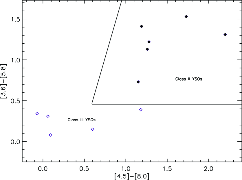
Figure 1: [3.6] - [5.8] vs. [4.5] - [8.0] color-color diagram for the data listed in Table 3.

In order to classify the sources in our sample, available IR photometry from 2MASS, IRAC and MIPS (Table 3) was examined via a slew of near- and mid-infrared color-color diagrams. Gutermuth et al (2005; 2008b; 2009) have shown that the [3.6] $-$ [5.8] vs. [4.5] $-$ [8.0] color-color diagram robustly classifies YSOs as either Class II or Class III, as well as filtering out background contaminants. The equations developed by Gutermuth et al. (2009) for the detection of YSOs in the Spitzer Young Cluster Survey were applied to the 15 sources in our sample with IRAC photometry. Figure 1 shows the [3.6] $-$ [5.8] vs. [4.5] $-$ [8.0] color-color diagram for the data listed in Table 3. Stars with the following color excesses:

$$[3.6]-[4.5]>0.7$$ (1)

and

$$[4.5]-[5.8]>0.7$$ (2)

are considered Class I YSOs because of their particularly flat or rising spectral energy distributions. Two sources in our sample, CXOANC J162727.0-244049 and CXOANC J034359.7+321403, were identified as Class I YSOs using these constraints.

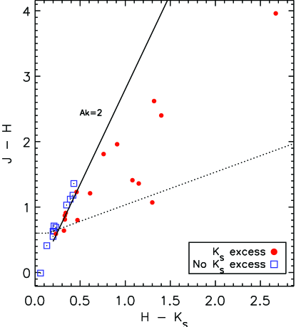
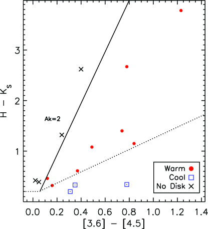
Figure 2: 2MASS band color-color diagrams for the data listed in Table 3 indicating the presence of a warm circumstellar disks.

The J $-$ H vs. H $-$ $K_{s}$ diagram shown in Figure 2 detects warm, massive disks that can be easily distinguished from the host star because they are optically thick at K-band. The J $-$ H vs. H $-$ $K_{s}$ diagram does not detect cooler disks that are not optically thick at K-band and thus have less contrast against the host star. The H - $K_{s}$ vs. [3.6] - [4.5] diagram also shown in Figure 2 detects massive but slightly cooler disks that may not be evident in the J $-$ H vs. H $-$ $K_{s}$ diagram. Warm disks may be ascribed to stars obeying all of the following constraints (Gutermuth et al. 2009):

$$for~{}[H-K]\leq 0.14,[J-H]=0.6$$ (3)

$$for~{}[H-K]>0.14,[J-H]=0.58\times[H-K]+0.52$$ (4)

$$for~{}[[3.6]-[4.5]]\leq 0.06,[H-K]=0.2$$ (5)

$$for~{}[[3.6]-[4.5]]>0.06,[H-K]=1.33\times[[3.6]-[4.5]]+0.133$$ (6)

In addition to six sources already classified with the IRAC 4-band plot, the J $-$ H vs. H $-$ $K_{s}$ diagram indicates that four additional YSOs possess warm disks. Ages less than 3 Myr for the stars in the host clusters are consistent with the presence of a disk. Both the J $-$ H vs. H $-$ $K_{s}$ and H $-$ $K_{s}$ vs. [3.6]$-$ [4.5] diagrams are included in Figure 2. Cold gas and dust at a distance of about 3 to 5 AU from the star emits brightly at 24$\mu$m  (Muzerolle et al. 2004). Accordingly, excess emission ($>$1.5 mag) in the [5.8] $-$ [24] and [4.5] $-$ [24] colors without associated excesses at shorter wavelengths is generally attributed to the absence of an inner disk and identifies stars with disks that are cold (i.e. transition disks), although other configurations such as rings are possible as well (Calvet et al. 2008). Source CXOANC J032929.2+311834 showed excess 24 $\mu$m  emission and no corresponding excess in either the [4.5] $-$ [5.8] or [3.6] $-$ [4.5] colors and so is identified as having a transition disk. Further YSO classifications were obtained from literature searches for six of the ten sources whose IR photometry did not conclusively place them in an evolutionary class. Several studies were consulted for these data (Flaccomio et al. 2006 for NGC 2264 – obsid 2540, Giardino et al.  2008 for NGC 752 – obsid 3752; Kohno et al. 2002 for Mon R2 – obsid 1882; Damiani et al. 2004 for NGC 6530 – obsid 977; Dahm & Hillenbrand 2007 for NGC 2362 and M8 – obsids 4469 and 3754 respectively).

3 Flare Modeling

3.1 The Hydrodynamic Model of Stellar Flares

Modeling the spectra for each source is a multi-step procedure guided by the principle that flares are isolated events periodically altering an underlying characteristic spectrum – even if the underlying spectrum is composed of multiple unresolved flares. Because the coronae of stars in our dataset are unresolved, the key to determining flare characteristics is good modelling of the spectra of the quiescent, peak and decay segments of the flare. The model itself has evolved over about 20 years, beginning with the thermodynamic timescale for flare loop decay of Serio et al. (1991) as a function of loop half-length $L$ (considered from one of the flare footpoints to its apex), peak temperature $T_{PK}$, and e-fold decay time $\tau_{TH}$:

$$\tau_{TH}=3.7\times 10^{-4}{L\over{\sqrt{T_{PK}}}}$$ (7)

In principle, if $T_{PK}$ and $\tau_{TH}$ can be determined, equation 7 can be inverted to obtain the flare loop length. However, the quantities $\tau_{TH}$ and $T_{PK}$ cannot be directly observed. Instead, they must be derived based on other observable quantities from the data.

Because the archetypal flares’ rise time is significantly shorter than the decay time, $\tau_{TH}$ in equation 7 assumes impulsive heating concentrated only at the beginning of the flare event. If the heating is not strictly impulsive, the flare plasma may be subject to prolonged heating extending into the decay phase. As a result, the flare’s e-fold decay time measured directly from the light curve ($\tau_{LC}$) would be longer than the flare’s intrinsic decay time ($\tau_{TH}$) and application of equation 7 would result in the overestimation of flare loop length. The slope of the flare plotted in a log T vs. log $n_{e}$ space ($\zeta$) can be used as a quantitative measure of the timescale of any sustained heating. Reale et al. (1997) show that $\zeta$ provides a diagnostic of the ratio between intrinsic ($\tau_{TH}$) and observed decay times ($\tau_{LC}$) such that:

$${\tau_{LC}\over{\tau_{TH}}}=F(\zeta)$$ (8)

The actual form of $F(\zeta)$ is observation-specific, depending on the band-pass and spectral response of the instrument used to obtain flare data. For values of $\zeta$ between 0.32 and 1.5, the ratio between observed and intrinsic flare times for ACIS observations has been calibrated to:

$${\tau_{LC}\over{\tau_{TH}}}=F(\zeta)={0.63\over{\zeta-0.32}}+1.41$$ (9)

Equation 9 allows for the substitution of $\tau_{TH}$ in Equation 7 with the observable quantities $\tau_{LC}$ and $\zeta$. Favata et al. also calibrated the actual peak flare temperature, $T_{PK}$, as a function of the observed temperature (in kelvins), $T_{OBS}$, for ACIS observations:

$$T_{PK}=0.068\times T_{OBS}^{1.2}$$ (10)

With corrections for sustained heating and instrumental response in place, the equation for flare loop half-length is based entirely on observable quantities and becomes:

$$L={\tau_{LC}\sqrt{T_{PK}}\over 3.7\times 10^{-4}F(\zeta)}$$ (11)

The loop length, in turn, may be used to determine the volume of the flare loop. If the ratio $\beta$ between the flare’s radius and its length is fixed at the solar value of $\beta\sim 0.1$, then the volume of the flare loop may be derived using equation (8) from Favata et al. :

$$V=2\pi\beta^{2}L^{3}$$ (12)

Consequently, we can infer the flare’s resulting plasma density in cm^-3 and confining magnetic field($B$) in gauss using equations (9) and (10) from Favata et al. by estimating the electron density ($n_{e}$):

$$n_{e}=\sqrt{{EM\over V}}=\sqrt{{EM\over 2\pi\beta^{2}L^{3}}}$$ (13)

$$B=\sqrt{(8\pi)(kn_{e}T_{PK})}$$ (14)

where, through the Ideal Gas Law, the quantity $kn_{e}T$ is equivalent to the flare loop’s plasma pressure. It should be noted that this estimate of the magnetic field is actually a lower limit, only the minimum field strength required to confine plasma of density $n_{e}$ and temperature $T_{PK}$. The flare’s confining magnetic field may be higher than inferred from equation 14. Equations 11, 13, and 14 were applied to all sources in our sample; the resulting values of $L$, $B$ and $n_{e}$ are listed in Table 4. Uncertainty in the value of $\beta$ used to derive $B$ and $n_{e}$ introduces considerable systematic error into their reported values, and so the calculated values for the magnetic field and the electron density should be understood to represent relative magnitudes. Assuming an extreme case of a circular flare loop for which $\beta=1$, the estimates differ by a factor of 10 for the electron density and a factor of 3 for the magnetic field.

It should be noted that this formulation for stellar flares is degenerate in that it doesn’t differentiate between a single long flaring loop and an arcade of several smaller flaring loops for a given length of plasma. Such complex flaring structures have been observed on the Sun, and they can have very simple light curves. Because the sources in our sample are unresolved, it is impossible to distinguish between a single flare loop and an arcade of smaller loops.

3.2 Application of Model to X-ray Data

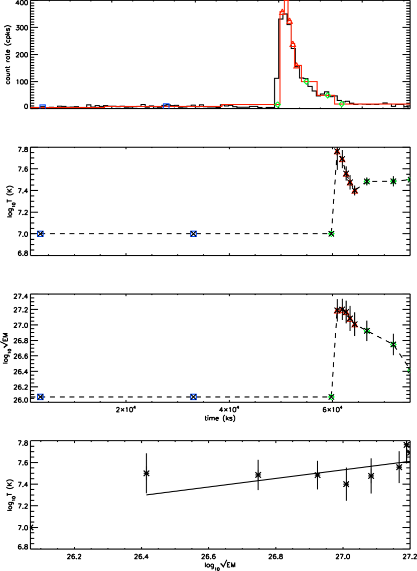
Figure 3: Flare analysis described in §3 as applied to an archetypal flare, CXOANC J182943.0+010207 (Chandra observation 4479). The topmost plot is the light curve for the source. Segments considered at the characteristic level are plotted as blue squares, rise and decay segments are plotted as green diamonds, and peak flare segments are plotted as red triangles. The next two plots show the evolution of the flare’s temperature and emission measure with time. The bottom plot shows the evolution of the flare in the log $T$ - log$\sqrt{EM}$ plane, with the points used to obtain $\zeta$ connected by a best-fit line (the characteristic point on the lower left is excluded).

To ascertain $\zeta$ and so characterize the flare loop, resolved spectra of each phase of the flare are required. In order to obtain these phase-resolved spectra, the light curve of each source is divided into a characteristic portion, a peak potion, and a decay portion. A finer resolution on the flare translates to a better-constrained value for $\zeta$ and more confident derivation of flare characteristics, so the peak and decay portions of the light curve are themselves subdivided into multiple segments. Light curve subdivision relies on timing information from the Bayesian blocks (BBs) generated with the Scargle (1998) algorithm and a prior consistent with 95% confidence that the photon arrival rate had changed. Depending on the particular resolution of the source, there can be as few as three or as many as nine individual segments associated with a flare event on a star in our sample. Each segment of a flare event was required to have a minimum of 100 to 150 counts, and in all cases $N_{\rm H}$ was fixed to the value reported in the ANCHORS database, usually of order $10^{22}$ cm^-3. This limits uncertainties in temperature to less than 30%. We assume that the $N_{\rm H}$ is dominated by interstellar gas or material associated with the local disk, not material associated with possible coronal mass ejections or accretion streams. The subdivision of the lightcurve into segments is shown for a sample source (Chandra observation 4479) in the topmost plot of Figure 3.

After subdivision, spectra are generated for all flare event segments with the specextract routine from CXC’s CIAO 3.4 software package. The resulting spectra are fitted with an absorbed multi-temperature model using Sherpa 2.0 to obtain the evolution of temperature and density needed for the calculation of flare parameters. Because Sherpa fits are based on chi-squared minimization, the spectra are binned to ensure robust statistics.

Spectral fits occur in several steps. First, the characteristic spectrum is fitted with a three-temperature model with all abundances freed in order to provide the best possible fit to the data. The model assumes the emission spectrum of collisionally ionized diffuse thermal plasma as calculated with the APEC code (Smith et al. 2001). To account for the interstellar medium and the circumstellar environment of the sources, a multiplicative absorption component (WABS; Morrison & McCommon 1982) is included in the model. Initial guesses for hydrogen column density came from the ANCHORS estimate. We assume that the gas column is dominated by interstellar gas or material associated with the local disk, not material associated with a possible coronal mass ejection or possible accretion streams. The results of this stage of modeling have limited physical significance, but generally provide an excellent fit to the data and serve as a mathematical representation of the characteristic level from which evolution in density and temperature may be studied. After a model is determined for the characteristic spectrum, all parameters associated with it are frozen.

To fit the peak and decay segments of the flare event with the frozen characteristic model, we include another component consisting of a simple one-temperature APEC model with only temperature and normalization as free parameters. The frozen portion of this new, compound model represents the underlying characteristic level, while the one-temperature component monitors changes in temperature and emission measure associated with the flare. The compound model was fitted to each segment of all flare events in our sample. Normalizations from the fits are interpreted as emission measures for the particular segment of the light curve. This stage of modeling leads to a series of points tracking the evolution of a flare in temperature and density (via the proxy of $\sqrt{EM}$). The two middle plots of Figure 3 show this evolution for Chandra observation 4479.

We then calculate $\zeta$ and subsequently the sustained heating correction $F(\zeta)$ for all sources in our sample by fitting the slope of $\log T$ vs. $\log\sqrt{EM}$ (see the bottom of Figure 3 for an example). Finally, loop lengths and other derived quantities are determined for the flare events in our sample through application of equations 9 through 14.

It should be noted that our procedure closely follows the analysis of Favata et al. (2005) but does not replicate it exactly: differences in the sample selection techniques, light curve subdivision, etc., could potentially affect derived characteristics for the flare. In order to calibrate and verify our implementation, we processed source 1246 from the COUP survey (Favata et al. 2005). We derived a value of 1.03$\pm$ 0.21 for $\zeta$, which agrees within uncertainty to the value of 0.90 $\pm$ 0.18 reported by Favata et al. Our loop half-length of $50\times 10^{10}$ cm (with a range of $43-55\times 10^{10}$ cm) is also consistent the value of $40\times 10^{10}$ cm reported by Favata et al. ($37-47\times 10^{10}$ cm). All other derived flare characteristics agree to within a factor of about 2. Infrared photometry for COUP 1246 is included in Table 3, and its derived flare characteristics are included in Table 4.

4 RESULTS

Table 4 summarizes the physical characteristics of the flares inferred from the analysis in §3, and includes the energy released by the entire flare event and the YSO class of the sources when it is known. The total energy released by a flare event was calculated as follows: for each segment of the flare modeled, the APEC/WABS model outputs an X-ray flux as well as temperature and emission measure. Multiplying this flux by the duration of the segment and scaling by the distance to the source yields the energy emitted by that particular flare segment. Summing over all segments modeled yields the total energy emitted by a flare. The $log_{10}$ of the average energy emitted by all flares in this sample is $35.7\pm 0.7$ ergs. The average energy emitted by flares on known Class II sources is $36.4\pm 0.8$ ergs, while flares on known Class III YSOs emit an average of $36.0\pm 0.5$ ergs. These two values agree within uncertainties and we conclude that the presence of a circumstellar disk does not appear to affect total energy emitted by a flare.

Figure 4 shows plots of the relationships among derived flare characteristics. Although the longer flares in this sample tend to be hotter and release more energy, flare temperature and emitted energy themselves are not strong predictors of loop length (fig. 4b,  4d), a result also seen by Getman et al. (2008a). As predicted by equation 11, flare loop length is more or less proportional to the square root of temperature, but significant scatter is introduced by the $F(\zeta)$ parameter measured from the data itself. Flare temperature and emitted energy are weakly correlated, with a Pearson $r$-coefficient of $0.52$ (fig. 4f). Equation 13 predicts that plasma density varies with the square of the magnetic field strength, a result we confirmed in Figure 4e.

As seen in Figures 4c and 4e, flare loop length is anti-correlated with magnetic field strength and plasma density; the longest flares in this sample are tenuous and weakly confined. In fact, Figures 4c and 4e suggest that flare loops longer than $1\times 10^{11}$ cm require magnetic fields weaker than 200 G and plasma density less than $5\times 10^{11}$ cm^-3. Although this observed dependence of loop length on magnetic field strength and plasma density is predicted by equations 11, 13, and 14, the trends shown in Figures 4c and 4e are not guaranteed by the model: the reported flare properties depend on emission measure and peak flare temperature, quantities which are determined from the data and do not depend on the hydrodynamic model described in this section.

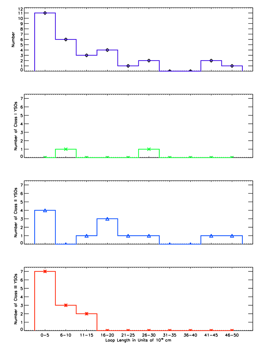
Figure 5: Loop length of flares sorted by IR class. The uppermost plot shows the distribution of loop lengths for all IR classes, including unclassified YSOs (represented as black circles). The Class I YSOs are represented by green crosses, the Class II YSOs by blue triangles, and the Class III YSOs by red asterisks.

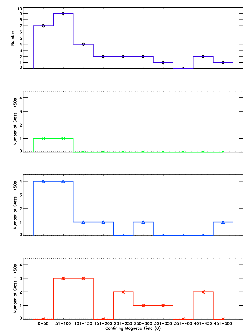
Figure 6: Flare confining magnetic field strength sorted by IR class. In the uppermost plot, the distribution of magnetic field strengths for all IR classes is shown, including unclassified YSOs. Colors and symbols are the same as Figure 5.

Histograms of derived flare characteristics segregated by source YSO class are shown in Figures 5 through 8. The loop length histogram shows that about two–thirds of the sources in our sample have loop lengths equal to or smaller than the stellar radius (assuming that $R_{\star}=3R_{\odot}$, cf. Baraffe et al. 1998). About half of the flares in the sample are “hot,” with peak plasma temperatures exceeding 100 MK. Figures 6 and  8 show that about two–thirds of flare events in our sample are confined in magnetic fields less than 150 G, and about 90% of the flares have plasma density less than $2\times 10^{12}$ cm^-3.

We now examine differences in the flare characteristic histograms by YSO class in order to determine the effect of circumstellar disks on flaring behavior. Figure 5 shows that while the distribution of the twelve identified Class II YSOs’ loop lengths is fairly spread out over all bins out to $5\times 10^{11}$ cm, none of the eleven identified Class III YSOs has a loop length longer than $1.3\times 10^{11}$ cm. To quantify this result, the distributions of loop lengths were compared using a two-sided Kolmogorov-Smirnov (KS) tests. We assumed that the molecular envelopes of material in-falling onto outer parts of a disk associated with Class I YSOs would have no effect on flaring behavior, so the Class I distribution was combined with the Class II distribution to test whether the presence of thick circumstellar disks affects flare loop length. Comparing the Class III loop length distribution to the ensemble of Class I and Class II loop lengths with a KS test yields an 11% probability that the two distributions are drawn from the same parent population. Though not definitive, this result is suggestive of a difference between Class I/II and Class III YSOs in the mechanism(s) driving at least some flare production.

Kolmogorov-Smirnov tests are also used to quantify the magnetic field distributions seen in Figure 6. As a general rule, Class I YSOs observed in X-rays tend to be hotter than Class II and III YSOs, and since magnetic fields associated with flares vary as $\sqrt{T}$ (cf. equation 14), we expect the magnetic field strength distributions to reflect this difference. The KS statistic for the magnetic field strength distributions of identified Class II and Class III YSOs yields a 97% probability that the magnetic field strength distributions originate in the same parent population. We then compared the combined the Class II and Class III distributions with the magnetic field distribution of identified Class I YSOs. The resulting probability that the Class II/III distribution is drawn from the same parent population as the Class I distribution is only 0.7%. Although the Class I distribution comprises only two soures, the KS statistic at least suggests that the magnetic fields of Class I YSOs are quantitatively different from those on Class II and III YSOs.

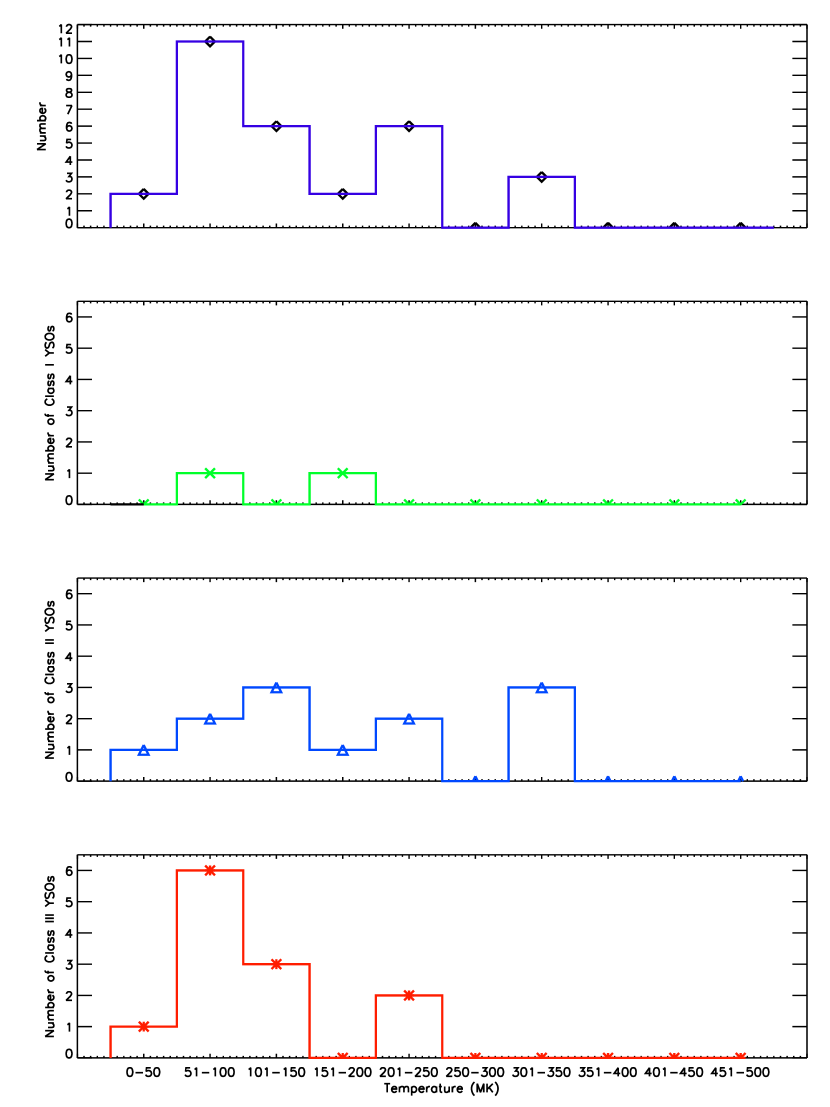
Figure 7: Peak flare temperature sorted by IR class. The uppermost plot shows the distribution of peak flare temperatures for all IR classes, including unclassified YSOs. Colors and symbols are the same as Figure 5.

Figures 7 and 8 show the distribution of peak flare event temperatures and plasma densities by YSO class. “Hot” flares with $T_{PK}>100$ MK are not observed preferentially to arise on a particular YSO class; a KS test on the set of temperatures results in a $98\%$ probability that the Class II and Class III temperature distributions originate in the same parent distribution. However, the two flares in our sample with $n_{e}>30\times 10^{10}$ $cm^{-3}$ occur on Class III YSOs. These findings are consistent with Figure 4b and  4c, which indicate that loop length is not a strong predictor of peak temperature but is rather anti-correlated with plasma density. Even if lengthened flares are preferentially found on Class II YSOs, the hottest flares will not necessarily be found on Class II YSOs as well.

As discussed in $\S 2.1$, our sample has a bias towards the brightest flares on young stellar objects. It is of interest to estimate the frequency with which these intense flares occur. By multiplying the number of sources in each Chandra observation included in our sample by the reported exposure time and summing over all observations, this sample may be estimated to contain approximately 2.9 million ks (i.e. $2.9\times 10^{9}$ seconds) of “on star” time. Twenty-nine large flares were observed in this “on star” time, which translates to one large flare per 100,000 ks of observation time. Phrased differently, the average YSO in our sample produces one of these intense flares, characterized by fast rise to a ten-fold increase in flux over the characteristic level followed by a smooth quasi-exponential decay, about once every three years.

5 Discussion

5.1 The Role of Disks in Flare Behavior

Lengths of the flaring structures in this sample range from $0.53\times 10^{10}$ cm to $50\times 10^{10}$ cm, ($\sim 0.03-3.0R_{\odot}$; assuming a fiducial $R_{\star}=3R_{\odot}$). Their confining magnetic fields range between tens and hundreds of Gauss. Compact flares with $L\leq 0.5R_{\star}$ could easily be contained within the YSOs’ dipole fields and appear similar to coronal events seen on ZAMS or MS stars. Compact flares have been frequently observed on YSOs, which led to the historical modeling of YSO magnetic fields as enhanced solar-type magnetic fields with footpoints anchored in the stellar photosphere (cf. Feigelson & Montmerle 1999 and references therein). While explaining the compact flares on YSOs, the enhanced solar-type model cannot account for the long magnetic structures (of order several stellar radii) implied by the most extended flare events in our sample. Without an enormous field tension as a counterbalance, the centrifugal force on magnetic structures several stellar radii long and anchored solely on the stellar surface would likely be sufficient to rupture the loops and eject any plasma before flaring. Moreover, for the long loops in our sample, the data do not support the existence of the high magnetic field tension expected in a tightly wound arcade of flares. In fact, as shown in Figure 4a, loop length is anti-correlated with confining magnetic field.

Confronted with the failure of the enhanced solar-type model to explain long flares, the most probable magnetic field geometry capable of supporting coherent magnetic fields over several stellar radii is the connection of the stellar photosphere to the inner edge of the circumstellar disk via magnetic flux tubes.

Several theoretical models (e.g., Shu et al. 1993, 2000; Feigelson et al. 2006) predict that PMS stars are magnetically coupled to the inner edge of their (Keplerian) disks at corotation radii defined as

$$R_{c}=\sqrt[3]{{GM\over\Omega^{2}_{o}}}$$ (15)

Theoretical studies (Uzdensky et al. 2002; Matt & Pudritz 2005) indicate that the presence of a disk truncates the stellar magnetosphere so closed magnetic loops cannot extend much further into the accretion disk than this corotating inner edge. The steady state solution dictates that the inner edge of the accretion disk rotates at the same rate as the star, but dissipative effects lead to differential rotation between the stellar photosphere and the inner edge of the disk. This differential rotation induces shearing of the long magnetic field lines connecting the star and disk, producing the stressed magnetic field configuration necessary to drive flares (Shu et al. 2000).

In typical low-mass PMS stars with rotation periods ranging from 2-10 days (cf. Edwards et al. 1993), equation 15 predicts an $R_{C}$ of about $3-5R_{\star}$ from the stellar surface. The radius from the star at which dust sublimates may be modelled as

$$R_{s}=\frac{\sqrt{Q_{R}}}{2}\left(\frac{T_{\star}}{T_{s}}\right)^{2}R_{\star}$$ (16)

where $T_{s}$ is the dust sublimation temperature and $Q_{R}$ is the ratio of the absorption efficiencies for dust at the color temperature of the incident and remitted radiation fields (Tuthill, Monnier & Danchi 2001). For a dust sublimation temperature of 1500 K, and a dust absorption efficiency $Q_{R}$ of 1, the sublimation radii range from 2$R_{\star}$ for a stellar temperature of 3000 K to 8$R_{\star}$ for a stellar temperature of 6000 K. D’Alessio et al. (2004) add a term to equation 16 which accounts for luminosity from any accretion streams. This extra luminosity may push the dust sublimation radius up to three times further out from the star, but its inclusion requires detailed infrared spectra to constrain the radiation field and dust opacities. As such, we do not attempt to estimate the contribution to the stellar radiation field due to accretion streams. It may be of interest to calculate dust destruction radii for the two flares in our sample in which star-disk interaction is the most likely. For J182016.5-161003, with flare loop length $4.4\times 10^{11}$ cm, there is no reliable radius or temperature estimates available. Assuming a Siess model-based $R_{\star}=3R_{\odot}$ for a stellar mass between 0.2 and 3$M_{\odot}$, and a corresponding effective temperature of 4000 K, equation 16 yields an inner disk edge of $7.4\times 10^{11}$ cm from the star, which likely out of reach of the flare. If a model temperature of 3075 K is used, equation 16 yields a dust sublimation radius of $4.5\times 10^{11}$ cm and flare-disk interaction becomes probable. The case for flare-disk interaction in J182016.5-161003 remains ambiguous. For the second long flare, COUP 1246 with flare loop length $5.0\times 10^{11}$, Favata et al. (2005) publish a mass of 0.2 $M_{\odot}$ and a stellar radius of 1.6 $R_{\odot}$. Using a corresponding Siess model temperature of 4000 K, the corresponding dust destruction radius is $4.0\times 10^{11}$ cm, which is easily within reach of the flare.

Five of the 14 flares in our sample associated with disked YSOs have $L\leq 0.5R_{\star}$, much like the flares described by Pandey & Singh (2008) on active evolved stars. Compact flares can be wholly contained by the YSO’s dipole field regardless of the presence of circumstellar accretion disks; for this reason compact flares are generally considered analogous to coronal events seen on ZAMS or MS stars. The wide range of loop lengths in the sample suggests that either of two types of flares may occur on disked YSOs: compact flares – analogous to flares on evolved stars – or long and the result of star-disk magnetic connections.

Star-disk magnetic coupling can explain the YSO class-specific distribution of loop lengths seen in Figure 5. The disks of Class I and II YSOs have inner radii close to surface of the central star and are thus far more likely to support the extended magnetic structures of star-disk coupling than the meager or non-existent disks associated with Class III YSOs. If star-disk magnetic coupling drives long flares we should not see any long flares associated with Class III YSOs. The loop length histograms of Figure 5 are evidence for the existence of star-disk magnetic coupling, as flares longer than $1.5\times 10^{11}$ cm are only observed on Class I and II YSOs.

From these results and the results published in the COUP survey (§5.2), a consistent picture of star-disk magnetic interaction in YSOs emeges. As part of normal chromospheric activity on a young star, the local magnetic field is arranged in arcade loops analagous to those seen on the Sun. Convection on the surface of the star causes shuffling of the loop footprint, which eventually stresses the magnetic field loops and causes a reconnection event and flare. Since YSOs have large surfaces compared to Sun-like MS stars, convective activity (and shuffling of the arcade loop footprint) is comparatively reduced. If the surface underneath the loop footprint is calm enough, and if they are equatorially located, the magnetic loops can grow large enough to interact with the inner edge of disk by drawing out ionized material. The presence or absence of a circumstellar disk plays no role in determining high-contrast flare energetics, but should a field line reach out and find disk material, the disk supports this extended magnetic structure and the accompanying extended high-contrast flare once the flux tube ruptures. For a detailed discussion of scenarios in which magnetic field loops can grow to several stellar radii, see MacNeice et al. (2004).

Such extended high-contrast flares are rare. There are 4 candidates in our sample of 12 Class II YSOs, which suggests that these kinds of flares occur once a decade on a given Class II YSO. However, as we note in §5.2, our sample is not sensitive to flares with $e$–fold cooling times longer than about half a day. Equation 11 implies that the $e$–fold cooling time is proportional to flare loop length, so our sample is effectively biased towards more compact flares, and the rate of occurence of extended flares may be higher by a factor of a few.

Twelve of the the thirty flares in our sample occur on disked Class II YSOs, and another twelve are detected on Class III YSOs. The total flare rate on Class II and Class III YSOs is consistent with being the same, with no significant observational bias between the two classes. This is further evidence that the flux flares in our sample are part of the normal variety of stellar flares: extended flares simply erupt in such a configuration that they can interact with the disk. Flares that reach the disk are not a separate variety of flare, but rather a special case of a more common (if large) flare.

5.2 Comparison to Other Flare Samples

The derived flare characteristics presented in Table 4 can be compared to results for the six late-type active evolved dwarfs studied by Pandey and Singh (2008), which used a similar technique for flare analysis. The six stars in their sample were observed for 30 to 60 ks, during which time Pandey and Singh report a total of 17 flares occurred. Flares in their sample do not last longer than 10 ks and usually only last a matter of minutes. Although the electron densities are similar in both our samples, the total energy released by flares in the sample of Pandey and Singh tend to be about three orders of magnitude smaller than the energy emitted by flares in our sample. Pandey and Singh conclude that flares in their sample are analogous to solar arcade flares; the numerous differences between the flares seen on the active dwarfs and the YSO flares indicate that unique influences must be driving the special case of long flares seen on Class II YSOs.

A comparison of the derived flare characteristics presented in Table 4 to the COUP survey’s flare characteristics (see Favata et al. 2005, Table 1) shows some global differences: the flare e-fold decay times in this study (mean of 11.0 ks) are significantly shorter than those reported in the COUP survey (mean of 67 ks); the dependence of derived flare characteristics on $\tau_{LC}$ leads to smaller loop lengths in our sample than those reported by Favata et al. The mean loop length in our sample is $14\pm 10\times 10^{10}$ cm and the mean magnetic field is $152\pm 106$ G compared to $103\pm 80\times 10^{10}$ cm and $351\pm 300$G respectively in the Favata et al. sample. This discrepancy may be explained in terms of differences in exposure times between the two studies. The average effective exposure time in our sample is 96 ks, with a maximum exposure time of 151 ks, significantly less than the unequaled 850 ks effective exposure time in the COUP survey. Our sample is effectively biased against flares lasting longer than  75-100 ks, which restricts $\tau_{LC}$ and thus the loop length (equation 11). Consequently, the flares in our sample tend to be shorter than flares in the COUP sample, which has no such restriction on $\tau_{LC}$.

In §4 we estimate the rate of occurrence of high-contrast flares in our sample to be 1 per 100,000 ks of exposure time. The COUP sample comprises 1500 stars nominally observed for 850 ks, but the effective COUP exposure time is actually somewhat longer than 850 ks because flares may occur during the 14-hour gaps between observations (when Chandra passes through the Van Allen belt) and still be detected by their aftereffects. With a revised effective exposure time of about 1130 ks, using our metric for rate of occurence we expect 17 high-contrast flare detections in the COUP sample. However, Favata et al. report 32 flare detections. This difference can be explained in several ways. First, the median age of stars in the ONC is only about 1 Myr, while the median age for stars in our sample is a slightly more mature 2.5 Myr, with some stars as old as 10 Myr. The younger stars in the ONC might simply be more active and produce more high-contrast flares. A difference in flare selection criteria between our two samples could also affect the number of flares reported. Favata et al. required only that three contiguous MLBs (see §2.1) be significantly elevated above the characteristic level and that the decay in the log T - log $\sqrt{EM}$ plane be sufficiently regular (i.e. monotonically decreasing). Our selection criteria were somewhat more exacting: in addition to requiring a linear decay in the log T - log $\sqrt{EM}$ plane, we required the archetypal flare behavior of fast rise and exponential decay with a peak count rate around 10 times the characteristic level.

We can also compare our sample of flares to the study published by Getman et al. (2008a,b). Getman et al. constructed a sample of 216 flares observed during the COUP mission and analyzed them using a different flare spectral analysis technique (MASME) that avoids nonlinear modeling (Getman et al. 2008a and references therein). The same hydrodynamic modeling used in §3 was used to derive flare properties like loop length and peak flare temperature. The selection criteria for flares in the Getman et al. sample were somewhat more relaxed than those used in this study: all flare morphologies, not just archetypal fast-rise-slow-decay flares, were accepted as long as the peak count rate was $\geq 4$ times that of the characteristic level. Sample selection aside, many of the derived flare properties are comparable to the results presented in Table 4: Getman et al. report a median $T_{OBS}$ of 63 MK, which is similar to our median $T_{OBS}$ of 50 MK, and a median loop length of $43\times 10^{10}\rm\,cm^{-2}$ for their sample. While the median loop length in our sample is only $10\times 10^{10}\rm\,cm^{-2}$, only two of the thirty flares in our sample have lengths equal to or greater than $43\times 10^{10}\rm\,cm^{-2}$; the difference in median loop lengths is likely due to our smaller sample size. Finally, Getman et al. conclude that disk presence has no effect on peak flare luminosity and total flare energy (2008b), a result which we confirm in §4.

The principle difference between our study and Getman et al. regards the role of disks in flaring behavior. As discussed in §5.1, we find that long flares of order $R_{C}$ occur only on disked PMS stars and conclude that in the case of these very long flares, one footpoint of the magnetic loop must be anchored on the accretion disk. Getman et al. come to the opposite conclusion, observing flares of order $R_{C}$ or longer almost exclusively on YSOs categorized as Class III in their study (2008b). While Getman et al. find little actual variation in flare properties between disked and diskless stars, they argue that due to their faster rotation periods, Class III YSOs actually have significantly smaller co–rotation radii than Class II YSOs and so regardless of length in cm, flares on Class II YSOs rarely if ever reach the disk and are anchored on the stellar photosphere alone.

Finally, we can compare our sample to the study of COUP flares recently published by Aarnio et al. (2010). Their goal was to understand the role that circumstellar disks play in the energetics of high-contrast X-ray flares. The authors construct spectral energy distributions in the wavelength range  0.3 $-$ 8 $\mu$m (extending in some cases out to 24 $\mu$m) and model them to determine whether there is circumstellar disk material in sufficient proximity to the flares’ confining magnetic loops to allow star-disk interaction. If $R_{\star}$, $M_{\star}$ and $T_{eff}$ are supplied, SED modelling can yield disk parameters including mass and sublimation radius. This technique characterizes the circumstellar disk more quantitatively than the near-infrared color excesses used in this study and has the advantage of detecting even cool disks with large inner holes. Aarnio et al. conclude that 58% of the stars in their COUP high-contrast flare sample have no disk material within reach of the confining magnetic loops and so argue that high-contrast X-ray flares in general are purely stellar in origin, neither triggered nor stabilized by star-disk interactions. The authors further argue that as long as the confining magnetic field at the end of the loop is strong enough, the loop is stable even without being anchored on the disk. We agree that disk presence has no effect on flare energetics, however our Figure 4 shows that confining magnetic field falls off sharply with loop length irrespective of disk presence and does not support this scenario.

Aarnio et al. do agree that for 10 of objects studied, star-disk interaction is possible and that the IR photometry of a further 8 sources in the sample does not permit conclusive statements about disks. Of the 15 flares in their sample with loops longer than about 10 $R_{\star}$, 5 flares appear within reach of the inner edge of the disk, and another 5 fall into the unknown category and have flare loop lengths of order the dust destruction radius. While not all flares studied by Aarnio et al. require star-disk interaction, the longest flares in the COUP high-contrast flare sample could be stablized by a circumstellar disk in the scenario presented in §5.1.

5.3 Comparison to Superflares

We have already discussed the bias in this sample towards high luminosity flares; these intense flares on YSOs may be analogs to so-called “superflares” seen on magnetically active main sequence stars. Schaefer et al. (2000) apply the term “superflare” to flares with energies ranging from $10^{33}$ to $10^{38}$ ergs on main sequence stars of spectral class F8 to G8 with no close binary companion and no evidence for rapid rotation.

Osten et al. (2007) reported the detection of an X-ray superflare on the active binary system II Pegasi. The II Peg superflare radiated $6\times 10^{36}$ ergs, the vast majority of which was radiated at energies less than 10 keV (see figure 4 of Osten et al. 2007). This value is comparable to the average energy radiated by flares in our sample, $1.66\times 10^{36}$ ergs. It is thus tempting to draw an analogy between the YSO flares in our sample and superflares like those reported on II Peg, and so we can compare superflare characteristics to our flare sample. The reported II Peg superflare temperature is somewhat higher than observed (not peak) temperatures in our sample: various model fits to II Peg yield flare temperatures between 118 and 152 MK, consistent with the highest observed temperature in our sample of 126 $\pm$ 30 MK. The entire II Peg superflare only lasted for 11 ks, which is closer to the average e-fold decay time of flare events in our sample, not their entire duration. Based on 6.4 keV emission, Osten et al. report a loop length range of 0.5 $-$ 1.3 $R_{\star}$ for the superflare, which falls within the range of loop lengths observed in our sample, 0.2 $-$ 3 $R_{\star}$. Osten et al. use $n_{e}$ of about $10^{11}$ cm^-3, consistent with our sample’s median plasma density of $1.2\times 10^{11}$ cm^-3. Using the values for plasma density and observed temperature reported by Osten et al., equation 14 can be used to estimate that the II Peg superflare is confined by a magnetic field of about 50 G, which is also consistent with the magnetic field strengths observed in our sample. Finally, Osten et al. estimate that superflares like the one on II Pegasi occur once every 5.4 months, considerably more frequent than the value of one flare every three years calculated in §4 for our sample. Although similar flare characteristics do not guarantee identical flare production mechanisms, if II Peg may be considered representative of superflares on other active MS stars, such superflares seem analogous to the flares in our sample.

5.4 Iron 6.4 keV Fluorescence

Another important observation noted during the II Peg superflare was the detection of iron K-shell fluorescence emission at 6.4 keV (Osten et al. 2007). Fluorescence emission has been well documented for solar flares and has also been observed on several YSOs sources (Tsujimoto et al. 2005, Skinner et al. 2007, 2009). The line can penetrate a large column density (up to $10^{24}$ cm^-2) and so serves as an excellent probe of circumstellar environments. The existence of Fe K$\alpha$ emission on the Sun is usually attributed to photoexcitation of iron in the photosphere by bremsstrahlung radiation. A similar mechanism is believed to produce the emission on YSOs with two differences: the fluoresced iron is located in the circumstellar disk, not the photosphere, and the fluoresced material is irradiated by the X-rays from magnetic reconnection events, not quasi-stable stellar X-rays. Tsujimoto et al. report that detection of 6.4 keV emission line is correlated with larger-than-average flare amplitude, and they predict that 6.4 keV emission due to photoionization occurs exclusively in young stars with disks. The emission was reported in only 6 out of 127 sources examined by Tsujimoto et al. Careful examination of the 30 sources in our sample for the presence of 6.4 keV emission yielded no positive detection of the line. Our sample contains only 14 known Class I and II YSOs with disks thick enough for photoionized 6.4 keV, assuming the same rate of detection as seen by Tsujimoto et al. we would have expected only about a 50% probability of detecting an iron fluorescence line from one of our disked stars. Thus, zero detections in the 14 disked systems studied is consistent with their detection rate.

6 Conclusions

In this study, we built a sample of bright flare events on YSOs suitable for time-resolved spectral analysis from the ANCHORS database. We modeled the flare events with the time-dependent hydrodynamic model of Reale et al. (1997). The results of flare modeling were then examined in the context of YSO classification information from available near- and mid-infrared data. We identify large flares as having a fast rise in count rate to a level about ten times the characteristic level, followed by a slower quasi-exponential decay back down to characteristic level. We calculate that YSOs produce flares like the ones in our sample about once every three years. The flares in this sample exhibit a variety of plasma temperatures and loop lengths, but the more extended flares are tenuous and confined by weak magnetic fields. We find that flare loop length is anti-correlated with magnetic field strength and plasma density and that flare temperature and energy do not correlate with flare loop length, a result also noted by Getman et al. (2008b) and Aarnio et al. (2010). Flare properties derived in this study are comparable in magnitude to those presented by Getman et al. (2008a,b) and Aarnio et al. (2010) but significantly smaller than those presented by Favata et al. (2005). This discrepancy is most probably caused by the much longer observation time of sources in the COUP mission than in our sample, which allows for the discovery of more extended flares with longer decay times.

Comparison of the flares in our sample with a well-studied superflare on II Pegasi, a magnetically active main sequence star, reveals that although the peak flare temperature Class I and II YSOs, and the lack of loop lengths longer than $13\times 10^{10}$ cm on the identified Class III YSOs, suggests and energy emitted by the II Peg superflare is comparable to energies in our sample, the entire II Peg superflare event was relatively short. Overall, the the II Peg superflare is consistent with the compact flares in our sample, suggesting analagous flare production mechanisms. A search for 6.4 keV fluorescent iron emission as observed in the II Peg superflare in our sample yielded a null result. This was however, consistent with the number of stars in our sample and the generally observed low rate of detection.

The detection of flares of order several stellar radii in length on the existence of long magnetic structures connecting the star and disk. We suggest the following scenario for star-disk magnetic interaction: equatorially located magnetic loops like those seen on the Sun can grow large enough to interact with the inner edge of a circumstellar accretion disk, provided convection on the chromosphere does not shuffle the loop footprint too much. The presence of a circumstellar disk does not determine flare energetics, but should a field line reach out and find disk material, the disk supports this extended magnetic structure. When the magnetic loop ruptures due to, e.g., differential rotation between the star and the disk, an extended flare results. Star-disk magnetic coupling thus explains the distribution of loop lengths seen in Figure 4: the thin or non-existent disks associated with Class III YSOs cannot support the coherent magnetic field structures required for long flares. A limitation of the hydrodynamic model employed in this study is the inability to distinguish between a single large flare loop or an arcade of smaller loops for a given loop length L. However, we find it evidentiary that the only flares with L of order the dust destruction radius occur on stars with disks, and we do not find extended flare loop lengths for Class III sources. While these results are not conclusive proof of star-disk magnetic interaction, they are highly suggestive.

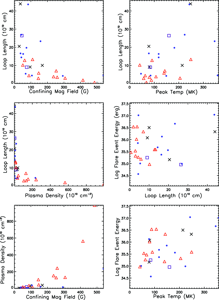
Figure 4: Plots of the relationships between the various flare characteristics presented in Table 4. Purple squares represent Class I YSOs, blue circles denote Class II YSOs, red triangles represent Class III YSOs, and unclassified YSOs are shown as black crosses.

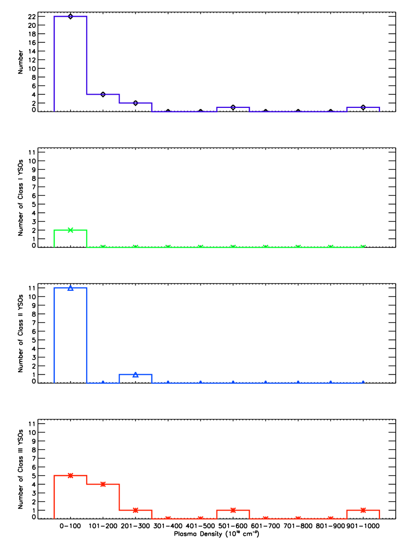
Figure 8: Flare plasma density sorted by IR class. In the uppermost plot, the distribution of plasma densities for all IR classes is shown, including unclassified YSOs. Colors and symbols are the same as Figure 5.

Table 1: X-ray properties of the 29 non-COUP sources used in this study.

ANCHORS ID	Off-axis distance	Counts	Counts	Aperture Flux	Luminosity	Hardness	Hardness	Hardness
						Ratio 1	Ratio 2	Ratio 3
[CXOANC …]	[arcsec]	[raw]	[net]
J162726.95-244049.8	406.0	2997	2979.0	-11.02	30.11	0.97	0.48	0.99
J162622.49-242252.0	1026.0	6824	6660.3	-10.60	30.59	0.92	0.75	0.99
J162715.46-242639.1	464.5	1271	1258.5	-11.39	29.70	0.94	0.70	0.99
J162624.10-242447.2	179.3	2246	2241.6	-11.07	30.18	0.96	0.80	1.00
J053456.83-051133.0	498.1	2341	2311.8	-11.52	30.59	-0.46	0.27	0.21
J053525.73-050949.3	253.7	1450	1444.7	-11.70	30.38	-0.25	0.50	0.37
J053629.62-045359.3	1248.3	1115	1039.1	-11.61	30.48	-0.14	0.22	0.09
J182028.37-161030.4	31.6	1786	1771.1	-11.61	31.83	0.58	0.94	0.94
J182041.14-161530.6	320.7	2015	2003.3	-11.44	32.01	0.71	0.91	0.99
J182016.54-161003.0	192.1	1006	1001.8	-11.54	31.90	0.99	0.01	0.99
J054131.61-015232.2	272.3	1341	1337.1	-11.43	30.54	0.50	0.89	0.96
J054148.22-015602.0	57.8	1636	1633.5	-11.17	30.83	0.97	0.69	1.00
J054145.07-015144.6	207.9	1679	1677.7	-11.24	30.75	0.84	0.94	0.99
J064113.15+092611.0	528.3	1442	1418.0	-11.57	31.03	-0.17	0.47	0.32
J064058.51+093331.7	42.9	3089	3086.3	-11.30	31.32	0.03	0.41	0.44
J064105.35+093313.3	115.4	2845	2841.9	-11.39	31.24	-0.02	0.43	0.42
J053523.47-051850.0	277.6	1267	1262.0	-11.47	30.72	-0.04	0.61	0.59
J164055.46-490102.6	783.4	1574	1403.1	-11.45	38.6	0.33	0.77	0.88
J032929.26+311834.6	377.2	1550	1544.2	-11.08	31.59	0.43	0.83	0.93
J015751.17+375257.0	421.1	2603	2583.7	-11.50	30.51	-0.41	0.15	0.28
J015751.43+375305.3	429.9	3971	3951.5	-11.35	30.67	-0.43	0.18	-0.27
J060732.35-061215.5	691.8	1479	1433.2	-11.49	31.15	0.26	0.81	0.89
J060814.11-062558.4	394.7	2222	2209.2	-11.23	31.44	0.64	0.88	0.97
J180438.93-242533.2	332.0	1227	1223.5	-11.41	31.62	0.22	0.68	0.79
J071845.24-245643.8	38.4	1510	1508.2	-11.59	31.55	0.04	0.51	0.54
J180402.88-242140.0	252.3	1893	1882.1	-11.63	31.38	0.00	0.58	0.58
J085932.21-434602.6	75.1	1675	1671.0	-11.20	31.86	0.80	0.92	0.99
J182943.01+010207.1	819.2	2830	2585.7	-11.29	30.36	0.25	0.76	0.85
J034359.71+321403.8	516.5	2222	2211.0	-11.02	30.85	0.26	0.79	0.87

Table 2: Log of the 17 Chandra observations used.

Pointing RA	Pointing Dec	Obs. ID	Target Name	Cluster Age	Cluster Dist.	Expos. Time	Obs. Start Date	Reference
				[Myr]	[pc]	[ks]
16:27:17.18	-24:34:39.0	635	Rho Oph. Core	0.3	130	101.87	Apr 13 2000	Imanshi et al. (2001)
16:26:34.20	-24:23:27.8	637	Rho Oph. A	0.3	130	97.6	May 15 2000	Imanshi et al. (2001)
05:35:19.98	-05:05:29.8	634	OMC 2/3	1	450	89.17	Jan 01 2000	Tsuboi et al. (2001)
18:20:20.29	-16:10:44.9	6420	M17 Pointing I	$<$ 1	2100	151.36	Aug 01 2006	Povich et al. (2009)
05:41:46.30	-01:55:28.7	1878	NGC 2024	1 $-$ 3	380	76.43	Aug 08 2001	Skinner et al. (2003)
06:40:58.10	+09:34:00.4	2540	NGC 2264	3	760	96.97	Oct 28 2002	Rebull et al. (2006)
05:35:15.00	-05:23:20.0	18	Trapezium Cluster	0.8 $-$ 1	450	47.44	Oct 12 1999	Garmire et al. (2000)
16:40:00.10	-48:51:45.0	4503	RCW 108	3	1300	9.96	Oct 25 2004	Wolk et al. (2008)
03:29:02.00	+31:20:54.0	6436	NGC 1333	1	300	36.95	Jul 05 2006	Winston et al. (2010)
01:57:39.00	+37:46:10.0	3752	NGC 752	1900	400	134.08	Sep 29 2003	Giardino et al. (2008)
06:07:49.50	-06:22:54.7	1882	Monoceros R2	6 $-$ 10	830	98.08	Dec 12 2000	Kohno et al. (2002)
18:04:24.00	-24:21:20.0	977	NGC 6530	2	400	60.93	Jun 18 2001	Damiani et al. (2004)
07:18:42.80	-24:57:18.5	4469	NGC 2362	5	1500	99.14	Dec 23 2003	Delgado et al. (2006)
18:03:45.10	-24:22:05.0	3754	M8	2	1300	129.60	Jul 25 2003	Arias et al. (2006)
08:59:27.50	-43:45:24.0	6433	RCW 36	2 $-$ 3	700	71.30	Sep 23 2006	Baba et al. (2004)
18:29:50.00	+01:15:30.0	4479	Serpens Cloud Core	$<$ 3	260	89.58	Jun 19 2004	Giardino et al. (2007)
03:44:30.00	+32:08:00.0	606	IC 348	2	320	52.96	Sep 21 2000	Preibisch & Zinnecker (2001)

Table 3: Available infrared photometry for the 30 flare events in the sample.

Chandra Obs ID	ANCHORS ID	YSO class	$A_{K_{s}}$	$J$	$H$	$K_{s}$	[3.6 $\mu$m]	[4.5 $\mu$m]	[5.8 $\mu$m]	[8.0 $\mu$m]	[24 $\mu$m]
	[CXOANC …]
635	J162727.0-244049	1	4.80	$\cdots$	13.52	9.74	6.71 1	5.48	4.57	3.80	$\cdots$
635	J162622.5-242251	2	0.28	16.45	15.09	13.94	12.39	11.55	10.86	9.82	5.78
635	J162715.5-242639	2	3.60	17.42	13.46	10.79	8.21	7.43	6.80	6.24	3.49
637	J162624.1-242447	2	1.69	11.12	8.72	7.32	5.63	4.89	4.41	3.61	1.23
634	J053456.8-051133	2	0.00	10.90	10.35	10.15	8.92	8.61	8.19	7.46	$\cdots$
634	J053525.7-050949	3	0.00	11.07	10.43	10.11	9.69	9.53	9.30	8.35	$\cdots$
634	J053629.6-045359	$\cdots$	$\cdots$	12.66	11.97	11.74	$\cdots$	$\cdots$	$\cdots$	$\cdots$	$\cdots$
6420	J182028.4-161030	$\cdots$	$\cdots$	13.77	12.41	11.98	$\cdots$	$\cdots$	$\cdots$	$\cdots$	$\cdots$
6420	J182041.1-161530	2	$\cdots$	15.48	13.52	12.61	$\cdots$	$\cdots$	$\cdots$	$\cdots$	$\cdots$
6420	J182016.5-161003	2	$\cdots$	16.11	15.04	13.74	$\cdots$	$\cdots$	$\cdots$	$\cdots$	$\cdots$
1878	J054131.6-015232	2	0.53	14.35	13.14	12.53	11.68	11.31	10.37	9.11	$\cdots$
1878	J054148.2-015602	3	4.39	$\cdots$	13.82	11.20	9.51	9.11	7.93	$\cdots$	$\cdots$
1878	J054145.1-015144	3	2.11	14.23	11.61	10.29	9.48	9.24	9.14	9.31	$\cdots$
2540	J064113.2+092610	2	$\cdots$	11.61	10.81	10.34	$\cdots$	$\cdots$	$\cdots$	$\cdots$	$\cdots$
2540	J064058.5+093331	$\cdots$	$\cdots$	10.22	10.23	10.17	$\cdots$	$\cdots$	$\cdots$	$\cdots$	$\cdots$
2540	J064105.4+093313	2	$\cdots$	12.48	11.85	11.64	$\cdots$	$\cdots$	$\cdots$	$\cdots$	$\cdots$
18	J053523.5-051849	3	0.26	11.99	11.12	10.79	10.61	10.26	8.98	$\cdots$	$\cdots$
4503	J164055.5-490102	3	0.67	13.11	11.88	11.42	11.21	11.09	10.90	11.03	$\cdots$
6436	J032929.2+311834	2/3	0.65	12.58	11.40	10.98	10.67	10.65	10.52	10.05	4.71
3752	J015751.2+375257	3	$\cdots$	12.01	11.38	11.18	$\cdots$	$\cdots$	$\cdots$	$\cdots$	$\cdots$
3752	J015751.4+375305	3	$\cdots$	10.11	9.70	9.57	$\cdots$	$\cdots$	$\cdots$	$\cdots$	$\cdots$
1882	J060732.4-061215	$\cdots$	$\cdots$	14.42	13.39	13.04	$\cdots$	$\cdots$	$\cdots$	$\cdots$	$\cdots$
1882	J060814.1-062558	2	0.43	12.51	11.10	10.02	8.45	7.96	7.32	6.70	3.11
977	J180438.9-242533	3	$\cdots$	14.26	13.45	13.12	$\cdots$	$\cdots$	$\cdots$	$\cdots$	$\cdots$
4469	J071845.2-245643	3	$\cdots$	15.06	14.47	14.24	$\cdots$	$\cdots$	$\cdots$	$\cdots$	$\cdots$
3754	J180402.9-242139	3	$\cdots$	11.98	11.27	11.06	$\cdots$	$\cdots$	$\cdots$	$\cdots$	$\cdots$
6433	J085932.2-434602	2	$\cdots$	14.42	12.61	11.85	$\cdots$	$\cdots$	$\cdots$	$\cdots$	$\cdots$
4479	J182943.0+010207	3	0.54	12.86	11.74	11.35	11.03	10.98	10.95	10.89	$\cdots$
606	J034359.7+321403	1	0.12	12.31	11.40	11.06	13.77	12.99	12.20	11.19	$\cdots$

Note. — IRAC photometry is all class A with average error of 0.01 magnitudes. Errors on the 2MASS photometry ranges from 0.03-0.1 magnitudes

Table 4: Calculated Flare Data

Obs ID	ANCHORS ID	$\tau_{LC}$	Max $T_{OBS}$	$T_{PK}$	$\zeta$	$\Delta~{}\zeta$	Loop Length	$n_{e}$	B	Tot Flare Energy
	[CXOANC …]	[$ks$]	[MK]	[MK]			[$10^{10}$ cm]	[$10^{10}~{}cm^{-3}$]	[$G$]	log[ergs]
Class I YSOs
635	J162727.0-244049	15.0	65	160	1.64	1.07	26.4 (26 $-$ 131)	3.7	45	34.96
606	J034359.7+321403	15.8	38	84	0.53	0.28	9.0 ($<$ 15)	18.8	74	35.25
Class II YSOs
635	J162622.5-242251	6.5	38	85	0.60	0.34	4.4 ($<$ 6.7)	38.1	106	34.56
635	J162715.5-242639	10.5	72	182	1.79	0.65	19.7 (17 $-$ 20)	8.4	73	35.56
637	J162624.1-242447	12.9	85	224	3.73	5.06	26.9 ( $\cdots$ )	2.3	42	34.99
634	J053456.8-051133	11.5	23	46	0.58	0.37	5.4 ($<$ 8.7)	2.9	68	35.00
2540	J064113.2+092610	9.5	50	118	2.01	3.10	14.4 ( $\cdots$ )	4.3	42	35.68
6420	J182041.1-161530	12.0	126	358	0.37	0.23	4.5 ($<$ 17)	234.0	539	37.01
6420	J182016.5-161003	20.7	91	243	1.39	0.73	43.6 (27 $-$ 45)	8.2	83	37.04
1878	J054131.6-015232	10.8	50	118	1.51	1.56	16.3 ( $\cdots$ )	6.9	53	35.37
2540	J064105.4+093313	23.5	36	78	0.64	0.21	16.6 (7.6 $-$ 21)	5.1	37	36.13
1882	J060814.1-062558	3.5	61	149	0.78	0.45	4.2 (0.13 $-$ 5.5)	16.5	293	35.85
6433	J085932.2-434602	9.0	123	346	2.36	1.43	23.3 (18 $-$ 24)	20.8	158	36.66
COUP 1246	$\cdots$	22.5	126	357	1.026	0.21	50.0 (43 $-$ 55)	2.0	50	$\cdots$
Class III YSOs
1878	J054148.2-015602	8.0	93	249	0.87	0.49	13.3 (3 $-$ 17)	14.0	110	35.59
1878	J054145.1-015144	19.0	40	91	0.58	0.43	12.8 ( $<$ 21)	12.0	62	35.59
4503	J164055.5-490102	6.4	39	88	0.41	0.45	1.9 ($<$ 6.2)	563.0	415	36.53
18	J053523.5-051849	2.5	32	68	0.4	0.12	0.6 ( $<$ 1.2)	990.0	485	35.47
3752	J015751.2+375257	7.5	27	57	0.49	0.213	2.9 ($<$ 5)	106.0	145	35.53
3752	J015751.4+375305	7.3	30	63	0.62	0.30	4.4 (0.07 $-$ 6)	35.4	88	35.27
634	J053525.7-050949	5.0	21	41	3.89	5.35	10.2 ( $\cdots$ )	18.4	51	34.97
4469	J071845.2-245643	8.8	46	107	0.44	0.20	3.8 ($<$ 7)	153.0	237	36.54
977	J180438.9-242533	4.8	59	143	1.11	0.88	7.0 ($<$ 8)	129.0	253	36.33
6436	J032929.2+311834	1.6	79	205	1.32	0.63	3.0 (2 - 3.2)	133.0	307	35.32
3754	J180402.9-242139	5.0	36	80	0.63	0.29	3.5 (0.53 $-$ 5)	242.0	259	36.02
4479	J182943.0+010207	3.5	58	140	1.92	1.35	5.8 (3 $-$ 6)	44.6	147	35.19
Unknown Class
6420	J182028.4-161030	7.5	82	214	0.72	0.71	10.0 ($<$ 15)	38.4	169	36.50
2540	J064058.5+093331	20.5	93	248	1.41	0.40	43.9 (37 $-$ 45)	1.5	36	36.33
1882	J060732.4-061215	17.0	36	80	0.52	0.24	9.1 ($<$ 15)	32.6	95	36.07
634	J053629.6-045359	22.5	36	78	0.84	0.36	20.5 (10 $-$ 25)	3.1	29	35.16

Note. — The flare loop lengths are presented with their uncertainty ranges in parentheses

References

- Aarnio et al. (2010) Aarnio, A. N., Stassun, K. G., & Matt, S. P. 2010, ApJ, 717, 93
- Arias et al. (2006) Arias, J. I., Barbá, R. H., Maíz Apellániz, J., Morrell, N. I., & Rubio, M. 2006, MNRAS, 366, 739
- Baba et al. (2004) Baba, D., et al. 2004, ApJ, 614, 818
- Caramazza et al. (2007) Caramazza, M., Flaccomio, E., Micela, G., Reale, F., Wolk, S. J., & Feigelson, E. D. 2007, A&A, 471, 645
- D’Alessio et al. (2004) D’Alessio, P., Calvet, N., Hartmann, L., Muzerolle, J., & Sitko, M. 2004, Star Formation at High Angular Resolution, 221, 403
- Dahm & Hillenbrand (2007) Dahm, S. E., & Hillenbrand, L. A. 2007, AJ, 133, 2072
- Damiani et al. (2004) Damiani, F., Flaccomio, E., Micela, G., Sciortino, S., Harnden, F. R., Jr., & Murray, S. S. 2004, ApJ, 608, 781
- Delgado et al. (2006) Delgado, A. J., González-Martín, O., Alfaro, E. J., & Yun, J. 2006, ApJ, 646, 269
- Edwards et al. (2003) Edwards, S., Fischer, W., Kwan, J., Hillenbrand, L., & Dupree, A. K. 2003, ApJ, 599, L41
- Favata et al. (2005) Favata, F., Flaccomio, E., Reale, F., Micela, G., Sciortino, S., Shang, H., Stassun, K. G., & Feigelson, E. D. 2005, ApJS, 160, 469
- Feigelson & Montmerle (1999) Feigelson, E. D., & Montmerle, T. 1999, ARA&A, 37, 363
- Feigelson et al. (2007) Feigelson, E., Townsley, L., Güdel, M., & Stassun, K. 2007, Protostars and Planets V, 313
- Fisk & Schwadron (2001) Fisk, L. A., & Schwadron, N. A. 2001, ApJ, 560, 425
- Flaccomio et al. (2006) Flaccomio, E., Micela, G., & Sciortino, S. 2006, A&A, 455, 903
- Garmire et al. (2001) Garmire, G., Feigelson, E. D., Broos, P., Hillenbrand, L. A., Pravdo, S. H., Townsley, L., & Tsuboi, Y. 2001, AJ, 120, 1426
- Getman et al. (2008a) Getman, K. V., Feigelson, E. D., Broos, P. S., Micela, G., & Garmire, G. P. 2008, ApJ, 688, 418
- Getman et al. (2008b) Getman, K. V., Feigelson, E. D., Micela, G., Jardine, M. M., Gregory, S. G., & Garmire, G. P. 2008, ApJ, 688, 437
- Giardino et al. (2007) Giardino, G., Favata, F., Micela, G., Sciortino, S., & Winston, E. 2007,å, 463, 275
- Giardino et al. (2008) Giardino, G., Pillitteri, I., Favata, F., & Micela, G. 2008, A&A, 490, 113
- Gregory & Loredo (1992) Gregory, P. C., & Loredo, T. J. 1992, ApJ, 398, 146
- Gutermuth et al. (2008) Gutermuth, R. A., et al. 2008, ApJ, 674, 336
- Gutermuth et al. (2009) Gutermuth, R.A., Megeath, S. T., Meyers, P. C., Allen, L. E., Pipher, J. L., & Fazio, G. G. 2009, ApJS, 184, 18
- Hartmann (1994) Hartmann, L. 1994, NATO ASIC Proc. 417: Theory of Accretion Disks - 2, 19
- Hillenbrand (1997) Hillenbrand, L. A. 1997, AJ, 113, 1733
- Hillenbrand et al. (1998) Hillenbrand, L. A., Strom, S. E., Calvet, N., Merrill, K. M., Gatley, I., Makidon, R. B., Meyer, M. R., & Skrutskie, M. F. 1998, AJ, 116, 1816
- Hudson (1991) Hudson, H. S. 1991, Solar Physics, 133, 357
- Imanishi et al. (2001) Imanishi, K., Koyama, K., & Tsuboi, Y. 2001, ApJ, 557, 747
- Kohno et al. (2002) Kohno, M., Koyama, K., & Hamaguchi, K. 2002, ApJ, 567, 423
- Lada et al. (1976) Lada C. J., Gull T. R., Gottlieb C. A., & Gottlieb E. W. 1976, ApJ, 203, 159
- Liseu et al. (1992) Liseu, R., Lorenzetti, D., Nisini, B., Spinpglio, L., & Moneti, A. 1992, å, 265, 577
- MacNeice et al. (2004) MacNeice, P., Antiochos, S. K., Phillips, A., Spicer, D. S., DeVore, C. R., & Olson, K. 2004, ApJ, 614, 1028
- Matt & Pudritz (2005) Matt, S. & Pudritz, R. E. 2005, MNRAS, 356, 167
- Meyer et al. (1997) Meyer, M. R., Calvet, N., & Hillenbrand, L. A. 1997, AJ, 114, 288
- Morrison & McCammon (1983) Morrison, R., & McCammon, D. 1983, ApJ, 270, 119
- Osten et al. (2007) Osten, R. A., Drake, S., Tueller, J., Cummings, J., Perri, M., Moretti, A., & Covino, S. 2007, ApJ, 654, 1052
- Pandey & Singh (2008) Pandey, J. C., & Singh, K. P. 2008, MNRAS, 387, 1627
- Reale et al. (1997) Reale, F., Betta, R., Peres, G., Serio, S., & McTiernan, J. 1997, A&A, 325, 782
- Reale (2007) Reale, F. 2007, A&A, 471, 271
- Rebull et al. (2006) Rebull, L. M., Stauffer, J. R., Ramirez, S. V., Flaccomio, E., Sciortino, S., Micela, G., Strom, S. E., & Wolff, S. C. 2006, AJ, 121, 2934
- Povich et al. (2009) Povich, M. S., et al. 2009, ApJ, 696, 1278
- Scargle (1998) Scargle, J. D. 1998, ApJ, 504, 405
- Shu et al. (1993) Shu, F., Najita, J., Galli, D., Ostriker, E., & Lizano, S. 1993, Protostars and Planets III, 3
- Shu et al. (2001) Shu, F. H., Shang, H., Gounelle, M., Glassgold, A. E., & Lee, T. 2001, ApJ, 548, 1029
- Skrutskie et al. (2006) Skrutskie, M. F., et al. 2006, AJ, 131, 1163
- Serio et al. (2010) Serio, S., Reale, F., Jakimiec, J., Sylwester, B., & Sylwester, J. 1991, A&A, 241, 197
- Siess et al. (2000) Siess, L., Dufour, E., & Forestini, M. 2000, A&A, 358, 593
- Skinner et al. (2003) Skinner, S., Gagné, M., & Belzer, E. 2003, ApJ, 598, 375
- Skinner et al. (2007) Skinner, S. L., Simmons, A. E., Audard, M. & Güdel, M. 2007, ApJ, 658, 1144
- Skinner et al. (2009) Skinner, S. L., Sokal, K. R., Megeath, S. T., Güdel, M., Audard, M., Flaherty, K. M., Meyer, M. R., & Damineli, A. 2009, ApJ, 701, 710
- Smith et al (2001) Smith, R. K., Brickhouse, N. S., Liedahl, D. A., & Raymond, J. C. 2001, ApJ, 556, L91
- Sylwester et al. (1993) Sylwester, J., Sylwester, B., Jakimiec, J., Garcia, H. A., Serio, S., & Reale, F. 1993, Advances in Space Research, 13, 307
- Tsuboi et al. (2001) Tsuboi, Y., Koyama, K., Hamaguchi, K., Tatematsu, K., Sekimoto, Y., Bally, J., & Reipurth, B. 2001, ApJ, 554, 734
- Uzdensky et al. (2002) Uzdensky, D. A., Königl, A., & Litwin, C. 2002, ApJ, 565, 1205
- Winston et al. (2007) Winston, E., et al. 2007, ApJ, 669, 493
- Winston et al. (2010) Winston, E., et al. 2010, AJ, 140, 266
- Wolk et al. (2005) Wolk, S. J., Harnden, F. R., Jr., Flaccomio, E., Micela, G., Favata, F., Shang, H., & Feigelson, E. D. 2005, ApJS, 160, 423
- Preibisch & Zinnecker (2001) Preibisch, T., & Zinnecker, H. 2001, AJ, 122, 866