Singlet-triplet relaxation in SiGe/Si/SiGe double quantum dots

Abstract

We study the singlet-triplet relaxation due to the spin-orbit coupling assisted by the electron-phonon scattering in two-electron SiGe/Si/SiGe double quantum dots in the presence of an external magnetic field in either Faraday or Voigt configuration. By explicitly including the electron-electron Coulomb interaction and the valley splitting induced by the interface scattering, we employ the exact-diagonalization method to obtain the energy spectra and the eigenstates. Then we calculate the relaxation rates with the Fermi golden rule. We find that the transition rates can be effectively tuned by varying the external magnetic field and the interdot distance. Especially in the vicinity of the anticrossing point, the transition rates show intriguing features. We also investigate the electric-field dependence of the transition rates, and find that the transition rates are almost independent of the electric field. This is of great importance in the spin manipulation since the lifetime remains almost the same during the change of the qubit configuration from $(1,1)$ to $(2,0)$ by the electric field.

I INTRODUCTION

Spin-based qubits utilizing semiconductor quantum dots (QDs) are believed to be the prospective candidate for quantum information processing.loss ; hanson ; wiel ; reimann Recently, silicon QDs have attracted much attention due to their outstanding spin-related properties.culcer ; li ; prada ; pan ; liu ; shaji ; culcer2 ; xiao ; wang ; raith ; das ; podd ; lai ; wild ; reboredo ; shin ; lim ; thalakulam ; hu2 ; simmons Specifically, the hyperfine interaction can be reduced by isotopic purification.taylor The Dresselhaus spin-orbit coupling (SOC)dresselhaus is absent thanks to the bulk-inversion symmetry and the SOC induced by the interface-inversion asymmetry (IIA) is rather weak.vervoort ; vervoort2 ; nestoklon Moreover, the electron-phonon interaction, which plays an important role in spin relaxation, is much weaker than that in III-V semiconductor QDs since there is no piezoelectric interaction in silicon.li All these special properties together lead to a long decoherence time in silicon QDs, which is of great help in the process of coherent manipulation and information storage. Furthermore, the physics in silicon is considerably rich owing to the presence of the valley degrees of freedom. Silicon has sixfold degenerate conduction band minima, which can be splitted by either strain or confinement in quantum wells into two parts: a fourfold-degenerate subspace of higher energy and a twofold one of lower energy. The twofold degeneracy can be further lifted by a valley-splitting energy due to the interface scattering. The valley-splitting energy has a strong dependence on the confinement length of the structure.boykin ; friesen

Nowadays, spin qubits in silicon single and double QDs have been actively investigated.culcer ; li ; prada ; pan ; liu ; shaji ; culcer2 ; xiao ; wang ; raith ; das ; podd ; lai ; wild ; reboredo ; shin ; lim ; thalakulam ; hu2 ; simmons In silicon single QDs, we have studied the singlet-triplet (ST) relaxation by explicitly including the electron-electron Coulomb interaction and the multivalley effect. Our results in the Voigt configuration agree quite well with the recent experiment by Xiao et al..xiao Silicon double QDs, which have been proven very useful in exploiting the spin Coulomb blockade,taylor2 have also attracted much attention. Recently, Raith et al.raith studied the magnetic-field and interdot-distance dependences of spin relaxation in single-electron Si/SiGe double QDs. Li et al.li calculated the exchange coupling between the unpolarized triplet and the singlet on the basis of a large valley splitting. Culcer et al.culcer investigated the multivalley effect on the feasibility of initialization and manipulation of ST qubits, showing that the valley degree of freedom makes the physics of Si QDs quite different from that of single-valley ones. In their work, they analyzed the spectrum with the lowest few basis functions. As will be shown in this paper, these lowest basis functions are enough for the convergence of the energy spectrum under investigation, but are inadequate to study the ST relaxation time, similar to the situation of III-V semiconductor-based QDs.shen The relaxation rates calculated with these lowest basis functions and the convergent ones differ by about four orders of magnitude. Therefore, it is necessary to employ the exact-diagonalization approach with a large number of basis functions in order to have the correct ST relaxation rates. Moreover, the electron-electron Coulomb interaction, which is crucial to the energy spectra and the wavefunctions of the singlet and triplet eigenstates, was not explicitly calculated in the literature but rather given as a Hubbard parameter.li ; culcer ; das

In this work, we calculate the two-electron ST relaxation in SiGe/Si/SiGe double QDs by explicitly including the Coulomb interaction, the valley degree of freedom as well as the source of the ST relaxation, i.e., the SOCs.rashba ; nestoklon We employ the exact-diagonalization method to obtain the energy spectrum and the Fermi golden rule to calculate the spin relaxation rates.cheng ; shen Without losing generality, we focus on a large valley splitting case where the lowest singlet and three triplet states are all constructed by the lowest valley eigenstate. We investigate the double QD system with either a perpendicular magnetic field (the Faraday configuration) or a parallel one (the Voigt configuration). We find that the energy levels of the lowest singlet and three triplet states have a strong dependence on the external magnetic field and the interdot distance. The perpendicular magnetic field affects the energy levels mainly by the orbital effect and the Zeeman splitting while the parallel magnetic field only influence the energy levels via the Zeeman splitting due to the strong confinement along the growth direction. The interdot distance has a strong influence on the Coulomb interaction and the orbital energy. Besides, we also find that the transition rates of the channels among these four levels can be markedly modulated by the external magnetic field and the interdot distance. Moreover, from the dependences of the energy spectrum on the magnetic field and the interdot distance, we observe the anticrossing points between the singlet and one of the triplets. In the vicinity of the anticrossing point, the transition rates of the channels relevant to these two states present either a peak or a valley. Furthermore, we also study the effect of the electric field on the energy levels and the transition rates. With the increase of the electric field, we find that the configurations of the lowest four levels change from $(1,1)$ to $(2,0)$, where $(n,m)$ indicates the numbers of occupancy of the left and right dots. Very different from the magnetic-field and interdot-distance dependences, we find that the transition rates are almost independent of the electric field. This property is of great importance in the spin manipulation, since the lifetime remains almost unchanged during the variation of qubit configurations.

This paper is organized as follows. We set up the model and lay out the formalism in Sec. II. In Sec. III, we employ the exact-diagonalization method to calculate the energy spectrum and the Fermi golden rule to obtain the ST relaxation rates. We investigate the magnetic-field (in both the Faraday and Voigt configurations), the interdot-distance and the electric-field dependences of the transition rates. The features of the transition rates in the vicinity of the anticrossing points are also emphasized. Finally, we summarize in Sec. IV.

II MODEL AND FORMALISM

In our model, we choose the lateral confinement potential as $V_{c}(x,y)=\frac{1}{2}m_{t}\omega_{0}^{2}\{{\rm min}[(x-x_{0})^{2},(x+x_{0})^{2}]+y^{2}\}$ with $m_{t}$ and $\omega_{0}$ representing the in-plane effective mass and the confining potential frequency.fock ; darwin A schematic of the double QDs is shown in Fig. 1. The two dots are located at ${\bf R}_{R,L}=(\pm x_{0},0,0)$ with $2x_{0}$ being the interdot distance. Here $R$ and $L$ denote right and left, respectively. Along the growth direction $[001]$, $V_{z}(z)$ is applied within the infinite-depth well potential approximation. The single-electron Hamiltonian with magnetic field ${\bf B}=B_{\perp}\hat{\bf z}+B_{\|}\hat{\bf x}$ can be written as

$$H_{\rm e} = \frac{{P_{x}}^{2}+{P_{y}}^{2}}{2m_{t}}+\frac{{P_{z}}^{2}}{2m_{z}}+V({\bf r})+H_{\rm so}({\bf P})$$ (1)

$$\mbox{}+H_{\rm Z}+H_{\rm E}+H_{\rm v},$$

with $m_{z}$ representing the effective mass along the $z$ direction. $V({\bf r})=V_{c}+V_{z}$ and ${\bf P}={\bf p}+(e/c){\bf A}=-i\hbar{\mbox{\boldmath$\nabla$\unboldmath}}+(e/c){\bf A}$ with ${\bf A}=(-yB_{\perp},xB_{\perp},2yB_{\|})/2$. $H_{\rm so}$ stands for the SOC Hamiltonian, including both the Rashbarashba and IIAvervoort ; vervoort2 ; nestoklon terms. Then, one obtains

$$H_{\rm so}=a_{0}(P_{x}\sigma_{y}-P_{y}\sigma_{x})+b_{0}(-P_{x}\sigma_{x}+P_{y}\sigma_{y}),$$ (2)

where $a_{0}$ and $b_{0}$ represent the strengths of the Rashba and IIA terms, respectively. The Zeeman splitting is given by $H_{\rm Z}=\frac{1}{2}g\mu_{B}(B_{\perp}\sigma_{z}+B_{\|}\sigma_{x})$ with $g$ being the Landé factor. $H_{\rm E}=eEx$ is the electric field term with an electric field applied along the $x$ direction. Considering that four in-plane valleys have much higher energies, we only need to include two out-of-plane valleys in the calculation. These two valleys lie at $\pm\langle k_{0}\rangle$ along the $z$ axis with $\langle k_{0}\rangle=0.85(2\pi/a_{\rm Si})$. Here, $a_{\rm Si}=5.43~{}\mathring{\rm A}$ is the lattice constant of silicon.culcer $H_{\rm v}$ in Eq. (1) describes the couplingboykin ; friesen between these two valleys. For convenience, one uses the subscripts “$z$” and “$\bar{z}$” to denote the valley at $\langle k_{0}\rangle$ and the one at $-\langle k_{0}\rangle$, respectively.

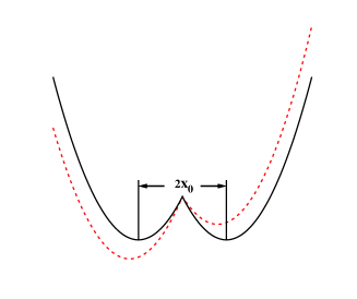
Figure 1: (Color online) Schematic of the double QDs. The black solid curve stands for the case without applied electric field. The red dotted curve represents the case with an electric field along the $x$ direction. $2x_{0}$ is the interdot distance.

To obtain the single-electron basis functions, we define $H_{0}=\frac{{P_{x}}^{2}+{P_{y}}^{2}}{2m_{t}}+\frac{{P_{z}}^{2}}{2m_{z}}+V({\bf r})$. The $z$-component of the Hamiltonian $H_{0}$ can be solved analytically with the eigenvalues being $E_{n_{z}}=\frac{{n_{z}}^{2}{\pi}^{2}{\hbar}^{2}}{8m_{z}a^{2}}$. Here $a$ represents the half-well width. The corresponding eigenfunctions are

$$\psi_{n_{z}}(z)=\left\{\begin{array}[]{ll}\frac{1}{\sqrt{a}}\sin[\frac{n_{z}\pi}{2a}(z+a)],&\mbox{$|z|\leq a$}\\ 0,&\mbox{otherwise}\end{array}\right.$$ (5)

in which the index $n_{z}$ stands for the subband along the growth direction. In our calculation, only the first subband is included since the others have much higher energies. It is very difficult to solve the in-plane part of $H_{0}$ analytically since the lateral confinement potential of the double QD, $V_{c}(x,y)$, lacks the symmetry of rotation. As the single-dot potential can be solved analytically,shen ; wang we solve the Hamiltonian of each dot separately instead to obtain the in-plane part of single-electron basis functions. We define $H_{L,R}=\frac{{P_{x}}^{2}+{P_{y}}^{2}}{2m_{t}}+\frac{1}{2}m_{t}\omega_{0}^{2}(x\pm x_{0})^{2}+\frac{1}{2}m_{t}\omega_{0}^{2}y^{2}$. The effective diameter can then be expressed as $d_{0}=\sqrt{\hbar\pi/(m_{t}\omega_{0})}$. In the left dot, $H_{L}=\frac{{P_{x}}^{2}+{P_{y}}^{2}}{2m_{t}}+\frac{1}{2}m_{t}\omega_{0}^{2}(x+x_{0})^{2}+\frac{1}{2}m_{t}\omega_{0}^{2}y^{2}=\frac{1}{2m_{t}}({p_{x^{\prime}}}^{2}+{p_{y}^{\prime}}^{2})+\frac{1}{2}m_{t}\Omega^{2}({x^{\prime}}^{2}+y^{2})+w_{B}(x^{\prime}{p_{y}^{\prime}}-yp_{x^{\prime}})$, where $x^{\prime}=x+x_{0}$, $p_{y}^{\prime}=p_{y}-w_{B}x_{0}m_{t}$, $\Omega=\sqrt{{\omega_{0}}^{2}+{\omega_{B}}^{2}}$ and $\omega_{B}={eB_{\perp}}/{(2m_{t})}$. We define $H_{L}^{\prime}=\frac{1}{2m_{t}}({p_{x^{\prime}}}^{2}+{p_{y}^{\prime}}^{2})+\frac{1}{2}m_{t}\Omega^{2}({x^{\prime}}^{2}+y^{2})$. One finds that the Hamiltonian $H_{L}$ can be solved analytically in the system of polar coordinates while $H_{L}^{\prime}$ can be solved analytically in the rectangular coordinate system.fock ; darwin As it is much easier to calculate the Coulomb interaction numerically in the rectangular coordinate system and the term $w_{B}(x^{\prime}{p_{y}^{\prime}}-yp_{x^{\prime}})$ can be treated perturbatively, we solve the Schrödinger equation of $H_{L}^{\prime}$ instead of $H_{L}$ to obtain the single-electron basis functions. One obtains the eigenvaluesfock ; darwin

$$E_{n_{x}n_{y}}=\hbar\Omega(n_{x}+n_{y}+1),$$ (6)

where $n_{x,y}=0,1,2,...$ are the orbital quantum numbers of the $x$ and $y$ direction, respectively. The eigenfunctions are described as

$$F_{n_{x}n_{y}}^{L}(x,y) = N_{n_{x}n_{y}}e^{-\alpha^{2}({x^{\prime}}^{2}+y^{2})/2}H_{n_{x}}(\alpha x^{\prime})H_{n_{y}}(\alpha y)$$ (7)

$$\mbox{}\times e^{iw_{B}x_{0}m_{t}y/\hbar}$$

with $N_{n_{x}n_{y}}=\{\alpha^{2}/[\pi(2^{n_{x}+n_{y}}n_{x}!n_{y}!)]\}^{1/2}$ and $\alpha=\sqrt{m_{t}\Omega/\hbar}$. $H_{n_{x},n_{y}}$ are the Hermite polynomials. Thus, the eigenfunctions in different valleys can be expressed as $\phi_{n_{x}n_{y}n_{z}}^{z,\bar{z},L}=F_{n_{x}n_{y}}^{L}(x,y)\Psi_{n_{z}}^{z,\bar{z}}({\bf r})=F_{n_{x}n_{y}}^{L}(x,y)\psi_{n_{z}}(z)e^{\pm ik_{0}z}u_{z,\bar{z}}({\bf r})$ with $u_{z,\bar{z}}({\bf r})$ representing the lattice-periodic Bloch functions.culcer Then one obtains a set of single-electron basis functions $\{\{\phi_{n_{x}n_{y}n_{z}}^{z,\bar{z},L}\},\{\phi_{n_{x}n_{y}n_{z}}^{z,\bar{z},R}\}\}$ where $\{\phi_{n_{x}n_{y}n_{z}}^{z,\bar{z},R}\}$ are the eigenfunctions in different valleys in the right dot and can be obtained by replacing $L$ and $x_{0}$ in the left dot by $R$ and $-x_{0}$. The orbital effect of the parallel magnetic field is negligible due to a strong confinement along the growth direction.

In the present work, only $H_{\rm v}$ is considered to contribute to the intervalley coupling since the overlap between the wavefunctions in different valleys is negligibly small.culcer However, there still remain some controversies over the valley coupling nowadays.friesen ; saraiva ; chutia Here, we take $\langle\Psi_{n_{z}}^{z,\bar{z}}|H_{\rm v}|\Psi_{n_{z}}^{\bar{z},z}\rangle=\Delta^{1}_{n_{z}}$ and $\langle\Psi_{n_{z}}^{z,\bar{z}}|H_{\rm v}|\Psi_{n_{z}}^{z,\bar{z}}\rangle=\Delta^{0}_{n_{z}}$ according to Ref. friesen, . Including this intervalley coupling, the single-electron eigenstates in the left dot become $\phi_{n_{x}n_{y}n_{z}}^{\pm L}=\frac{1}{\sqrt{2}}(\phi_{n_{x}n_{y}n_{z}}^{z,L}\pm\phi_{n_{x}n_{y}n_{z}}^{\bar{z},L})$ with eigenvalues $E_{n_{x}n_{y}n_{z}}^{\pm}=E_{n_{x}n_{y}}+E_{n_{z}}+\Delta_{n_{z}}^{0}\pm|\Delta_{n_{z}}^{1}|$. In these formulas,

$$\Delta_{n_{z}}^{0} = \frac{V_{\rm v}{n_{z}}^{2}{\pi}^{2}{\hbar}^{2}}{4m_{z}a^{3}},$$ (8)

$$\Delta_{n_{z}}^{1} = \frac{V_{\rm v}{n_{z}}^{2}{\pi}^{2}{\hbar}^{2}\cos(2k_{0}a)}{4m_{z}a^{3}},$$ (9)

with $V_{\rm v}$ representing the ratio of the valley coupling strength to the depth of quantum well.friesen For the case of the right dot, one can get the corresponding single-electron eigenvalues and eigenfunctions by replacing $L$ and $x_{0}$ in the left dot by $R$ and $-x_{0}$. Then one obtains a new set of single-electron basis functions $\{\{\phi_{n_{x}n_{y}n_{z}}^{\pm L}\},\{\phi_{n_{x}n_{y}n_{z}}^{\pm R}\}\}$. It is noted that these basis functions are nonorthogonal and over-complete.

Then we turn to the system of two-electron double QDs, where the total Hamiltonian is given by

$$H_{\rm tot}=(H_{\rm e}^{1}+H_{\rm e}^{2}+H_{\rm C})+H_{\rm p}+H_{\rm ep}^{1}+H_{\rm ep}^{2}.$$ (10)

Here, the two electrons are denoted by $``1"$ and $``2"$. The electron-electron Coulomb interaction is given by $H_{\rm C}=\frac{e^{2}}{4\pi\epsilon_{0}\kappa|{\bf r_{1}}-{\bf r_{2}}|}$ with $\kappa$ standing for the relative static dielectric constant. $H_{\rm p}=\sum_{{\bf q}\lambda}\hbar\omega_{{\bf q}\lambda}a_{{\bf q}\lambda}^{+}a_{{\bf q}\lambda}$ represents the phonon Hamiltonian with $\lambda$ and ${\bf q}$ denoting the phonon mode and the momentum, respectively. The electron-phonon interaction Hamiltonian is described by $H_{\rm ep}=\sum_{{\bf q}\lambda}M_{{\bf q}\lambda}(a_{{\bf q}\lambda}^{+}+a_{-{\bf q}\lambda})e^{i{\bf q}\cdot{\bf r}}$ and $H_{e}^{i}$ $(i=1,2)$ is given by Eq. (1).

On the basis of the set of single-electron basis functions $\{\{\phi_{n_{x}n_{y}n_{z}}^{\pm L}\},\{\phi_{n_{x}n_{y}n_{z}}^{\pm R}\}\}$, we construct the two-electron basis functions in the form of either singlet or triplet. For example, we use two single-electron spatial wavefunctions $|n_{x1}n_{y1}n_{z1}n_{v1}p_{1}\rangle$ and $|n_{x2}n_{y2}n_{z2}n_{v2}p_{2}\rangle$ (denoted as $|N_{1}\rangle$ and $|N_{2}\rangle$ for short; $n_{v}=\pm$; $p=L/R$) to obtain the singlet wavefunctions

$$|S^{(\Xi)}\rangle=(|\uparrow\downarrow\rangle-|\downarrow\uparrow\rangle)\otimes\begin{cases}\frac{1}{\sqrt{2}}|N_{1}N_{2}\rangle,&N_{1}=N_{2}\\ \frac{1}{2}(|N_{1}N_{2}\rangle+|N_{2}N_{1}\rangle),&N_{1}\not=N_{2},\end{cases}$$ (11)

and the triplet wavefunctions for $N_{1}\neq N_{2}$

$$|T_{+}^{(\Xi)}\rangle=\frac{1}{\sqrt{2}}(|N_{1}N_{2}\rangle-|N_{2}N_{1}\rangle)\otimes|\uparrow\uparrow\rangle,$$ (12)

$$|T_{0}^{(\Xi)}\rangle=\frac{1}{2}(|N_{1}N_{2}\rangle-|N_{2}N_{1}\rangle)\otimes(|\uparrow\downarrow\rangle+|\downarrow\uparrow\rangle),$$ (13)

$$|T_{-}^{(\Xi)}\rangle=\frac{1}{\sqrt{2}}(|N_{1}N_{2}\rangle-|N_{2}N_{1}\rangle)\otimes|\downarrow\downarrow\rangle.$$ (14)

Here, the spatial wavefunctions of the first and second electrons in $|NN^{\prime}\rangle$ are denoted as $N$ and $N^{\prime}$ in sequence. Specially, we denote $p_{1}=p_{2}=L/R$ as $(2,0)/(0,2)$ and $p_{1}\neq p_{2}$ as $(1,1)$ configuration. The superscript $(\Xi)$ denotes the valley configuration of each state. We define $\Xi=\pm$ for the valley indices of single electron states $n_{v1}=n_{v2}=\pm$, and $\Xi=m$ for $n_{v1}\neq n_{v2}$.

Then, one can calculate the matrix elements of two-electron Hamiltonian $H_{\rm e}^{1}+H_{\rm e}^{2}+H_{\rm C}$ in Eq. (10) and obtain the two-electron Hamiltonian matrix, where the matrix elements of the Coulomb interaction can be expressed by

$$\langle N_{1}N_{2}|H_{\rm C}|N_{1}^{\prime}N_{2}^{\prime}\rangle=\frac{e^{2}}{32{\pi}^{3}\epsilon_{0}\kappa}\sum_{\gamma_{1},\gamma_{2},\gamma_{1}^{\prime},\gamma_{2}^{\prime}=z,\bar{z}}\eta_{n_{v1}}^{\gamma_{1}}\eta_{n_{v2}}^{\gamma_{2}}\eta_{n_{v1}^{\prime}}^{\gamma_{1}^{\prime}}\eta_{n_{v2}^{\prime}}^{\gamma_{2}^{\prime}}G(\phi_{n_{x1}n_{y1}n_{z1}}^{\gamma_{1},p_{1}},\phi_{n_{x2}n_{y2}n_{z2}}^{\gamma_{2},p_{2}},\phi_{n_{x1}^{\prime}n_{y1}^{\prime}n_{z1}^{\prime}}^{\gamma_{1}^{\prime},p_{1}^{\prime}},\phi_{n_{x2}^{\prime}n_{y2}^{\prime}n_{z2}^{\prime}}^{\gamma_{2}^{\prime},p_{2}^{\prime}}),$$ (15)

where the superscripts $\gamma_{i}$ and $\gamma_{i}^{\prime}$ run over the two valleys, $z$ and $\bar{z}$, with $\eta_{\pm}^{z}=1$ and $\eta_{+}^{\bar{z}}=-\eta_{-}^{\bar{z}}=1$. $G$ is given by

$$G(\phi_{n_{x1}n_{y1}n_{z1}}^{\gamma_{1},p_{1}},\phi_{n_{x2}n_{y2}n_{z2}}^{\gamma_{2},p_{2}},\phi_{n_{x1}^{\prime}n_{y1}^{\prime}n_{z1}^{\prime}}^{\gamma_{1}^{\prime},p_{1}^{\prime}},\phi_{n_{x2}^{\prime}n_{y2}^{\prime}n_{z2}^{\prime}}^{\gamma_{2}^{\prime},p_{2}^{\prime}})=\int d^{3}{\bf k}\frac{\langle\phi_{n_{x1}n_{y1}n_{z1}}^{\gamma_{1},p_{1}}|e^{i{\bf k}\cdot{\bf r}}|\phi_{n_{x1}^{\prime}n_{y1}^{\prime}n_{z1}^{\prime}}^{\gamma_{1}^{\prime},p_{1}^{\prime}}\rangle\langle\phi_{n_{x2}^{\prime}n_{y2}^{\prime}n_{z2}^{\prime}}^{\gamma_{2}^{\prime},p_{2}^{\prime}}|e^{i{\bf k}\cdot{\bf r}}|\phi_{n_{x2}n_{y2}n_{z2}}^{\gamma_{2},p_{2}}\rangle^{*}}{k^{2}}$$ (16)

As two-electron basis functions are nonorthogonal, we also calculate the overlap between these basis functions. One finds that these two-electron basis functions can be divided into three independent subspaces according to the valley index, i.e., $\Xi=\pm$ and $m$, as there is nearly no couping between them due to the negligibly small intervalley Coulomb interactionli and overlap between the wave functions in different valleys.culcer Then one can diagonalize the eigen equation $\tilde{H}^{(\Xi)}X=\lambda\tilde{S}^{(\Xi)}X$ in each subspace separately and obtain corresponding two-electron energy spectra and eigenfunctions, where $\tilde{H}^{(\Xi)}$ and $\tilde{S}^{(\Xi)}$ stand for the two-electron Hamiltonian and overlap matrix in the subspace with the valley index $\Xi$ ($\Xi=\pm$ or $m$) respectively.lowdin We identify a two-electron eigenstate as singlet (triplet) if its amplitude of the singlet (triplet) components is larger than 50 %. We use the similar way to identify a two-electron eigenstate as $(2,0)$, $(0,2)$ or $(1,1)$ configuration according to the maximum amplitude.

The transition rate from the state $|i\rangle$ to $|f\rangle$ due to the electron-phonon scattering is calculated by the Fermi golden rule,

$$\Gamma_{i\rightarrow f} = \frac{2\pi}{\hbar}\sum_{{\bf q}\lambda}|M_{{\bf q}\lambda}|^{2}|\langle f|\chi|i\rangle|^{2}[\bar{n}_{{\bf q}\lambda}\delta(\epsilon_{f}-\epsilon_{i}-\hbar\omega_{{\bf q}\lambda})$$ (17)

$$\mbox{}+(\bar{n}_{{\bf q}\lambda}+1)\delta(\epsilon_{f}-\epsilon_{i}+\hbar\omega_{{\bf q}\lambda})],$$

in which $\chi({\bf q},{\bf r_{1}},{\bf r_{2}})=e^{i{\bf q}\cdot{\bf r_{1}}}+e^{i{\bf q}\cdot{\bf r_{2}}}$ and $\bar{n}_{{\bf q}\lambda}$ stands for the Bose distribution of phonons. In the calculation, the temperature is fixed at 0 K and only the second term, i.e., the phonon-emission process, occurs. One finds that the transition between the eigenstates in different subspaces is almost forbidden because $\langle f|\chi|i\rangle$ in Eq. (17) is strongly suppressed due to a large intervalley wave vector $\langle 2k_{0}\rangle$, similar to the suppressions of the intervalley Coulomb interaction and overlap between the wave functions in different valleys mentioned above.

III NUMERICAL RESULTS

From the Fermi golden rule [Eq. (17)], one finds that the phonon energy is just the energy difference between the initial and final electron states. The energy difference studied here is much smaller than the energies of the intervalley acoustic phonon and the optical phonon.pop Besides, the piezoelectric interaction is absent in silicon,li therefore one only needs to take into account the intravalley electron-acoustic phonon scattering due to the deformation potential. In this work, both the TA and LA phonons are included. The corresponding matrix elements read $M_{\beta,{\rm intra},{\bf Q}}^{2}={\hbar D_{\beta}^{2}Q^{2}}/{(2d\Omega_{\beta,{\rm intra},{\bf Q}})}$ with $\beta$=LA/TA representing the LA/TA phonon mode. The deformation potentials for the LA and TA phonons are $D_{{\rm LA}}=3.93$ eV and $D_{{\rm TA}}=2.48$ eV, respectively.pop The mass density of silicon $d=2.33$ g/cm³.sonder The phonon energy $\Omega_{\beta,{\rm intra},{\bf Q}}=v_{\beta}Q$ with sound velocities $v_{\rm LA}=9.01\times 10^{5}$ cm/s and $v_{\rm TA}=5.23\times 10^{5}$ cm/s.pop The effective mass $m_{t}=0.19m_{0}$ and $m_{z}=0.98m_{0}$ with $m_{0}$ being the free electron mass.dexter The Landé factor $g=2$,graeff the ratio of the valley coupling strength to the depth of quantum well $V_{\rm v}=7.2\times 10^{-11}$ m,friesen and the relative static dielectric constant $\kappa=11.9$.sze In the previous work on silicon double QDs,li ; culcer ; das only the lowest few basis functions were included in the calculation. We find that these basis functions are enough for the convergence of the energy spectra, but inadequate in obtaining the correct transition rates. The energy spectra calculated with the lowest few basis functions and the convergent ones differ by about $0.1$ %, but the transition rates calculated with the lowest few basis functions differ by about four orders of magnitude from the convergent ones. Therefore, in our calculation, we employ the exact-diagonalization method with the lowest 1050 singlet and 3060 triplet basis functions to ensure the convergence of the eigenstates and the transition rates. It is noted that all the basis functions chosen are in the subspace with the valley index $``-"$ since we focus on the case of a large valley splitting where a large effective diameter is taken to make sure that the lowest singlet and triplet states under investigation are in the subspace with the valley index $``-"$. This choice does not lead to the loss of generality as states with different valley indices are nearly decoupled as pointed out above. It is also noted that the Coulomb interaction was treated as a Hubbard parameter $u$ in the previous works on silicon double QDs,li ; culcer ; das but in our work, it is explicitly calculated. One can obtain $u$ from our calculation, e.g., $u$ in the model by Culcer et al.culcer is determined to be about $23$ meV.

III.1 PERPENDICULAR MAGNETIC-FIELD DEPENDENCE

We first investigate the case of a perpendicular magnetic field. We take 32 monoatomic layers of silicon along the growth direction of the quantum well, corresponding to the well width $2a=4.344$ nm. According to Eq. (9), a large valley splitting $2|\Delta_{n_{z}}^{1}|=0.83$ meV is obtained. Then we choose the effective diameter $d_{0}=30$ nm. With an electric field 30 kV/cm along the growth direction, one obtains the strength of the Rashba SOC induced by this electric field $a_{0}=-6.06$ m/s and that of the IIA term $b_{0}=-30.31$ m/s.nestoklon

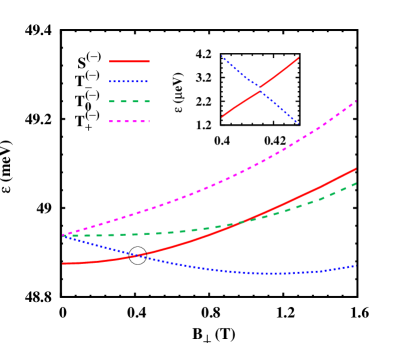
Figure 2: (Color online) The lowest four energy levels vs. perpendicular magnetic field $B_{\perp}$ in double QDs. The anticrossing point between $|S^{(-)}\rangle$ and $|T_{-}^{(-)}\rangle$ is shown and the range near this point is enlarged in the inset (the energies are substracted by $48.89$ meV). In the calculation, the interdot distance $2x_{0}=20$ nm.

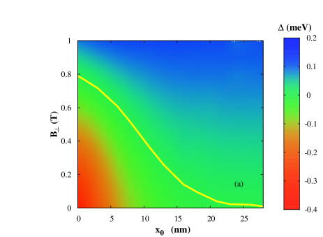
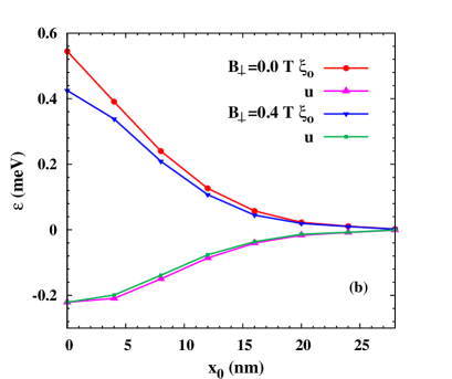
Figure 3: (Color online) (a) The energy difference between the lowest singlet $|S^{(-)}\rangle$ and the lowest triplet $|T_{-}^{(-)}\rangle$ vs. perpendicular magnetic field $B_{\perp}$ and half of the interdot distance $x_{0}$ in double QDs. The yellow solid cure is the position of the anticrossing between $|S^{(-)}\rangle$ and $|T_{-}^{(-)}\rangle$. (b) the orbital-energy difference between $|T_{-}^{(-)}\rangle$ and $|S^{(-)}\rangle$ $\xi_{o}$ and the energy difference of the Coulomb interaction $u$ vs. half of the interdot distance $x_{0}$ at zero magnetic field and a magnetic field $B_{\perp}=0.4$ T.

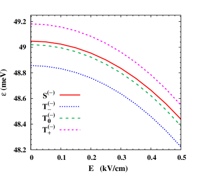
Figure 4: (Color online) The lowest four energy levels vs. electric field along the $x$ direction. In the calculation, the interdot distance $2x_{0}=20$ nm and the magnetic field $B_{\perp}=1.4$ T.

With the interdot distance $2x_{0}=20$ nm, the lowest four levels are plotted in Fig. 2 as function of the perpendicular magnetic field, denoted as $|S^{(-)}\rangle$, $|T_{+}^{(-)}\rangle$ (spin up), $|T_{0}^{(-)}\rangle$ (zero spin) and $|T_{-}^{(-)}\rangle$ (spin down) according to their major components. The energies of three triplet states are separated by the Zeeman splitting. From the figure, one finds that the singlet state $|S^{(-)}\rangle$ intersects with the triplet states $|T_{-}^{(-)}\rangle$ and $|T_{0}^{(-)}\rangle$ in sequence with the increase of the magnetic field. The intersecting point between $|S^{(-)}\rangle$ and $|T_{-}^{(-)}\rangle$ ($B_{\perp}\sim 0.415$ T) is an anticrossing point where there exists a small energy gap ($\sim 0.17$ $\mu{\rm eV}$) shown in the inset due to the Rashba SOCrashba and the IIA term.nestoklon The intersecting point between $|S^{(-)}\rangle$ and $|T_{0}^{(-)}\rangle$ ($B_{\perp}\sim 0.98$ T) is simply a crossing point.

The anticrossing between $|S^{(-)}\rangle$ and $|T_{-}^{(-)}\rangle$ can also be tuned by varying the interdot distance. We plot the energy difference between $|S^{(-)}\rangle$ and $|T_{-}^{(-)}\rangle$ as function of the magnetic field and the interdot distance in Fig. 3(a). In this figure, we also show the position of the anticrossing between $|T_{-}^{(-)}\rangle$ and $|S^{(-)}\rangle$. It is seen that the magnetic field where the anticrossing occurs decreases with the increase of the interdot distance. This can be understood from the energy difference between $|T_{-}^{(-)}\rangle$ and $|S^{(-)}\rangle$: $\Delta(B_{\perp},x_{0})=\xi_{o}+u-g\mu_{B}B_{\perp}$, where $\xi_{o}$ is the orbital-energy difference and $u$ comes from the contribution of the Coulomb interaction. By solving the equation $\Delta(B_{\perp},x_{0})=0$, one obtains the magnetic field $B_{\perp}^{c}$ corresponding to the anticrossing point. To facilitate understanding of the dependence of $B_{\perp}^{c}$ on the interdot distance, we plot the interdot-distance dependence of $\xi_{o}$ and $u$ at zero and a specific magnetic fields in Fig. 3(b). From this figure, one finds that the orbital-energy difference $\xi_{o}$ decreases with increasing the interdot distance while $u$, which is insensitive to the magnetic field under investigation, shows an opposite behavior. It is noted that the increase of $u$ is much smaller than the decrease of the orbital-energy difference $\xi_{o}$. Therefore, with the increase of the interdot distance, the net contribution of $\xi_{o}+u$ decreases and correspondingly the magnetic field where the anticrossing occurs, i.e., $B_{\perp}^{c}$, decreases too.

In addition, the electric field can also effectively affect the energy levels. We apply an electric field along the $x$ direction and plot the lowest four levels in Fig. 4. One notices that the energy levels are weakly dependent on the electric field in the small electric field regime but show a rapid decrease when the electric field becomes strong. This electric field dependence agrees with that reported by Culcer et al.culcer qualitatively. Moreover, one also finds that the energy differences among these levels are almost independent of the electric field. These behaviors can be understood as follows. With the increase of the electric field, the configuration of these four states gradually changes from $(1,1)$ to $(2,0)$ according to their major components. In $(1,1)$ configuration, i.e., in the small electric field regime, the electric field suppresses the single-electron energy in the left dot while raises it in the right dot. Therefore, the net contribution of the electric field is small and changes slowly with increasing electric field. However, when the electric field becomes strong, i.e., the states are in $(2,0)$ configuration, the energy of each electron decreases while that of the two-electron Coulomb interaction increases with increasing electric field. It is noted that the increase of the energy of the Coulomb interaction is much smaller than the decrease of the energies induced by the electric field. As a result, the energy levels show a rapid decrease. Besides, we find that these four states always keep the same configurations regardless of the strength of the electric field. Therefore, the electric field has the same effect on these states, leading to the energy differences among these levels insensitive to the electric field.

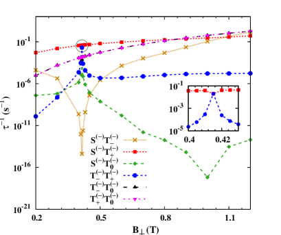
Figure 5: (Color online) Transition rates vs. perpendicular magnetic field. The inset zooms the range near the anticrossing point of the channels $S^{(-)}T_{+}^{(-)}$ and $T_{-}^{(-)}T_{+}^{(-)}$. In the calculation, the interdot distance $2x_{0}=20$ nm.

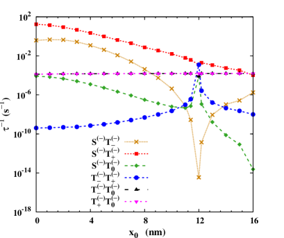
Figure 6: (Color online) Transition rates vs. half of the interdot distance. In the calculation, the magnetic field $B_{\perp}=0.3$ T.

We then calculate the ST relaxation rates together with the transition rates of the channels between two triplet states. From Fig. 5, one finds that the transition rates can be markedly modulated by the magnetic field. In the vicinity of the anticrossing point ($B_{\perp}\sim 0.415$ T), the transition rates show intriguing features. The rate between $|S^{(-)}\rangle$ and $|T_{-}^{(-)}\rangle$ shows a sharp decrease due to small phonon energy, which has been addressed in our previous investigations on GaAs and Si single QDs.shen ; wang The transition rates of other channels except the one between $|T_{+}^{(-)}\rangle$ and $|T_{0}^{(-)}\rangle$ present either a peak or a valley due to the large spin mixing between the singlet $|S^{(-)}\rangle$ and the triplet $|T_{-}^{(-)}\rangle$, similar to the behavior we have investigated in single QDs.wang Specifically, the transition rate between $|S^{(-)}\rangle$ and $|T_{+}^{(-)}\rangle$ and the one between $|T_{-}^{(-)}\rangle$ and $|T_{0}^{(-)}\rangle$ present a minimum while the transition rate between $|S^{(-)}\rangle$ and $|T_{0}^{(-)}\rangle$ and the one between $|T_{-}^{(-)}\rangle$ and $|T_{+}^{(-)}\rangle$ show a maximum. Far away from the anticrossing point, the variation of the transition rates can be well understood from the change of the phonon energy.climente ; shen ; wang

We also investigate the influence of the interdot distance on the ST relaxation rates together with the transition rates of the channels between two triplet states at $B_{\perp}=0.3$ T. The results are shown in Fig. 6. We also find an anticrossing point between $|S^{(-)}\rangle$ and $|T_{-}^{(-)}\rangle$ at $x_{0}\sim 12$ nm. In the vicinity of this point, the behavior of the transition rates is similar to what we have obtained above by sweeping the magnetic field. The transition rate between $|S^{(-)}\rangle$ and $|T_{-}^{(-)}\rangle$ is strongly suppressed and other transition rates relevant to these two states also show a rapid increase or decrease. Therefore, one can tune the ST relaxation by varying the interdot distance which can be controlled electrically in the experiment.

Moreover, the electric-field dependence of the transition rates is also studied. We find that the transition rates are almost independent of the electric field (not shown). This behavior can be understood from Fig. 4 where the energy differences among the lowest four levels are almost independent of the electric field.shen ; wang This property is of great importance in the spin manipulation, since the lifetime remains almost identical during the change of the qubit configuration from $(1,1)$ to $(2,0)$ by electric field.

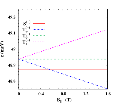
Figure 7: (Color online) The lowest four energy levels vs. parallel magnetic field $B_{\|}$ in double QDs. In the calculation, the interdot distance $2x_{0}=20$ nm.

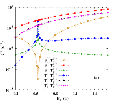
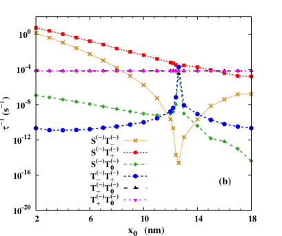
Figure 8: (Color online) (a) Transition rates vs. parallel magnetic field $B_{\|}$ with the interdot distance $2x_{0}=20$ nm. (b) Transition rates vs. half of the interdot distance with the magnetic field $B_{\|}=0.3$ T.

III.2 PARALLEL MAGNETIC-FIELD DEPENDENCE

We also investigate the case with a parallel magnetic field along the $x$ direction. The well width, effective diameter and strengths of both the Rashba SOC and the IIA term are chosen to be the same as the perpendicular magnetic-field case. We investigate the magnetic-field dependence of the energy spectrum in the absence of the applied electric field with the interdot distance $2x_{0}=20$ nm. The lowest four levels are plotted in Fig. 7. We denote these states as $|S^{(-)}\rangle$, $|T_{+}^{(-)}\rangle$, $|T_{0}^{(-)}\rangle$ and $|T_{-}^{(-)}\rangle$ according to their major components. From the figure, one finds that $|S^{(-)}\rangle$ and $|T_{0}^{(-)}\rangle$ are almost independent of the magnetic field while $|T_{+}^{(-)}\rangle$ and $|T_{-}^{(-)}\rangle$ show a linear dependence. This is because of the absence of the orbital effect of the parallel magnetic field thanks to a strong confinement along the growth direction. Therefore, the magnetic-field dependence is involved only through the Zeeman splitting. For $|S^{(-)}\rangle$ and $|T_{0}^{(-)}\rangle$, the $x$-components of the total spin are almost zero, leading to negligibly small Zeeman splitting. For $|T_{+}^{(-)}\rangle$ and $|T_{-}^{(-)}\rangle$, the $x$-components of the total spin are nearly $\pm 1$, which indicate that these two levels change linearly with the magnetic field. Besides, we also find an anticrossing point between $|S^{(-)}\rangle$ and $|T_{-}^{(-)}\rangle$ at $B_{\|}\sim 0.54$ T due to the SOCs.

The influence of the magnetic field and interdot distance on the ST relaxation rates is investigated. From Fig. 8, one finds that the behavior of the transition rates is quite similar to what obtained in the case of the perpendicular magnetic field. Here, one also observes the anticrossing point between $|S^{(-)}\rangle$ and $|T_{-}^{(-)}\rangle$ by sweeping the parallel magnetic field and/or interdot distance. In the vicinity of the anticrossing point, the transition rates relevant to these two states also show a rapid increase or decrease.

IV SUMMARY

In summary, we have investigated the ST relaxation in two-electron silicon double QDs with magnetic fields in both the Faraday and Voigt configurations. The electron-electron Coulomb interaction and the mutivalley effect are explicitly included. A large number of basis functions are utilized to converge the eigenstates and the transition rates. We find that the external magnetic field and the interdot distance have strong influence on the lowest four energy levels and consequently the transition rates can be effectively modulated by the external magnetic field and the interdot distance. Moreover, from the magnetic-field and interdot-distance dependences of the energy spectrum, we observe ST anticrossing points. In the vicinity of the anticrossing point, a small energy gap exists between the singlet and one of the triplet states due to the SOCs. The transition rates of the channels relevant to these two states show either a peak or a valley. Furthermore, we also study the effect of the electric field on the energy spectra and the transition rates. We find that the configuration of the lowest four levels change from $(1,1)$ to $(2,0)$ with the increase of the electric field. Differing from the magnetic-field and interdot-distance dependences, the transition rates are nearly independent of the electric field. This is of great importance in the spin manipulation since the lifetime remains almost unchanged during the manipulation of qubit configuration.

- (1) D. Loss and D. P. DiVincenzo, Phys. Rev. A 57, 120 (1998).
- (2) R. Hanson, L. P. Kouwenhoven, J. R. Petta, S. Tarucha, and L. M. K. Vandersypen, Rev. Mod. Phys. 79, 1217 (2007).
- (3) W. G. van der Wiel, S. De Franceschi, J. M. Elzerman, T. Fujisawa, S. Tarucha, and L. P. Kouwenhoven, Rev. Mod. Phys. 75, 1 (2002).
- (4) S. M. Reimann and M. Manninen, Rev. Mod. Phys. 74, 1283 (2002).
- (5) F. A. Reboredo, A. Franceschetti, and A. Zunger, Appl. Phys. Lett. 75, 2972 (1999).
- (6) S. J. Shin, J. J. Lee, R. S. Chung, M. S. Kim, E. S. Park, and J. B. Choi, Appl. Phys. Lett. 91, 053114 (2007).
- (7) M. Prada, R. H. Blick, and R. Joynt, Phys. Rev. B 77, 115438 (2008).
- (8) H. W. Liu, T. Fujisawa, Y. Ono, H. Inokawa, A. Fujiwara, K. Takashina, and Y. Hirayama, Phys. Rev. B 77, 073310 (2008).
- (9) N. Shaji, C. B. Simmons, M. Thalakulam, L. J. Klein, H. Qin, H. Luo, D. E. Savage, M. G. Lagally, A. J. Rimberg, R. Joynt, M. Friesen, R. H. Blick, S. N. Coppersmith, and M. A. Eriksson, Nat. Phys. 4, 540 (2008).
- (10) D. Culcer, L. Cywiński, Q. Li, X. Hu, and S. Das Sarma, Phys. Rev. B 80, 205302 (2009).
- (11) W. Pan, X. Z. Yu, and W. Z. Shen, Appl. Phys. Lett. 95, 013103 (2009).
- (12) W. H. Lim, H. Huebl, L. H. Willems van Beveren, S. Rubanov, P. G. Spizzirri, S. J. Angus, R. G. Clark, and A. S. Dzurak, Appl. Phys. Lett. 94, 173502 (2009).
- (13) B. Hu and C. H. Yang, Phys. Rev. B 80, 075310 (2009).
- (14) Q. Li, L. Cywiński, D. Culcer, X. Hu, and S. Das Sarma, Phys. Rev. B 81, 085313 (2010).
- (15) D. Culcer, L. Cywiński, Q. Li, X. Hu, and S. Das Sarma, Phys. Rev. B 82 155312 (2010).
- (16) M. Xiao, M. G. House, and H. W. Jiang, Phys. Rev. Lett. 104, 096801 (2010).
- (17) L. Wang, K. Shen, B. Y. Sun, and M. W. Wu, Phys. Rev. B 81, 235326 (2010).
- (18) G. J. Podd, S. J. Angus, D. A. Williams, and A. J. Ferguson, Appl. Phys. Lett. 96, 082104 (2010).
- (19) A. Wild, J. Sailer, J. Nützel, G. Abstreiter, S. Ludwig, and D. Bougeard, New J. Phys. 12, 113019 (2010).
- (20) M. Thalakulam, C. B. Simmons, B. M. Rosemeyer, D. E. Savage, M. G. Lagally, M. Friesen, S. N. Coppersmith, and M. A. Eriksson, Appl. Phys. Lett. 96, 183104 (2010).
- (21) C. B. Simmons, T. S. Koh, N. Shaji, M. Thalakulam, L. J. Klein, H. Qin, H. Luo, D. E. Savage, M. G. Lagally, A. J. Rimberg, R. Joynt, R. Blick, M. Friesen, S. N. Coppersmith, and M. A. Eriksson, Phys. Rev. B 82, 245312 (2010).
- (22) M. Raith, P. Stano, and J. Fabian, arXiv:1101.3858.
- (23) S. Das Sarma, X. Wang, and S. Yang, arXiv:1103.5460.
- (24) N. S. Lai, W. H. Lim, C. H. Yang, F. A. Zwanenburg, W. A. Coish, F. Qassemi, A. Morello, and A. S. Dzurak, arXiv:1012.1410.
- (25) J. M. Taylor, H.-A. Engel, W. Dür, A. Yacoby, C. M. Marcus, P. Zoller, and M. D. Lukin, Nat. Phys. 1, 177 (2005).
- (26) G. Dresselhaus, Phys. Rev. 100, 580 (1955).
- (27) L. Vervoort, R. Ferreira, and P. Voisin, Phys. Rev. B 56, R12744 (1997).
- (28) L. Vervoort, R. Ferreira, and P. Voisin, Semicond. Sci. Technol. 14, 227 (1999).
- (29) M. O. Nestoklon, E. L. Ivchenko, J.-M. Jancu, and P. Voisin, Phys. Rev. B 77, 155328 (2008).
- (30) T. B. Boykin, G. Klimeck, M. A. Eriksson, M. Friesen, S. N. Coppersmith, P. von Allmen, F. Oyafuso, and S. Lee, Appl. Phys. Lett. 84, 115 (2004).
- (31) M. Friesen, S. Chutia, C. Tahan, and S. N. Coppersmith, Phys. Rev. B 75, 115318 (2007).
- (32) J. M. Taylor, J. R. Petta, A. C. Johnson, A. Yacoby, C. M. Marcus, and M. D. Lukin, Phys. Rev. B 76, 035315 (2007).
- (33) K. Shen and M. W. Wu, Phys. Rev. B 76, 235313 (2007).
- (34) E. I. Rashba, Fiz. Tverd. Tela (Leningrad) 2, 1224 (1960) [Sov. Phys. Solid State 2, 1109 (1960)].
- (35) J. L. Cheng, M. W. Wu, and C. Lü, Phys. Rev. B 69, 115318 (2004).
- (36) V. Fock, Z. Phys. 47, 446 (1928).
- (37) C. G. Darwin, Proc. Cambridge Philos. Soc. 27, 86 (1931).
- (38) A. L. Saraiva, M. J. Calderón, X. Hu, S. Das Sarma, and B. Koiller, Phys. Rev. B 80, 081305(R) (2009).
- (39) S. Chutia, S. N. Coppersmith, and M. Friesen, Phys. Rev. B 77, 193311 (2008).
- (40) P. O. Löwdin, J. Chem. Phys. 18, 365 (1950).
- (41) E. Pop, R. W. Dutton, and K. E. Goodson, J. Appl. Phys. 96, 4998 (2004). It is noted that the deformation potentials for the LA and TA phonons and in this reference are incorrect, which was pointed out by Raith et al..raith In our calculation, the corrected and are taken. It is also noted that these parameters in our previous work on single QDs (Ref. wang, ) should also be adjusted. However, it is pointed out that the change of these parameters does not affect our results since the fitting parameters, i.e., the strengths of the Rashba SOC and the IIA term , can be changed correspondingly to obtain the identical results in our previous work.wang Specifically, in the parallel (perpendicular) magnetic-field case, can be changed from m/s ( m/s) to m/s ( m/s) and from m/s ( m/s) to m/s ( m/s).
- (42) E. Sonder and D. K. Stevens, Phys. Rev. 110, 1027 (1958).
- (43) R. N. Dexter, B. Lax, A. F. Kip, and G. Dresselhaus, Phys. Rev. 96, 222 (1954).
- (44) C. F. O. Graeff, M. S. Brandt, M. Stutzmann, M. Holzmann, G. Abstreiter, and F. Schäffler, Phys. Rev. B 59, 13242 (1999).
- (45) S. M. Sze, Physics of Semiconductor Devices (Wiley-Interscience, New York, 1981), p. 849.
- (46) J. I. Climente, A. Bertoni, G. Goldoni, M. Rontani, and E. Molinari, Phys. Rev. B 75, 081303(R) (2007).