An Interferometric and Spectroscopic Analysis
of the Multiple Star System HD 193322

Abstract

The star HD 193322 is a remarkable multiple system of massive stars that lies at the heart of the cluster Collinder 419. Here we report on new spectroscopic observations and radial velocities of the narrow-lined component Ab1 that we use to determine its orbital motion around a close companion Ab2 ($P=312$ d) and around a distant third star Aa ($P=35$ y). We have also obtained long baseline interferometry of the target in the $K^{\prime}$-band with the CHARA Array that we use in two ways. First, we combine published speckle interferometric measurements with CHARA separated fringe packet measurements to improve the visual orbit for the wide Aa,Ab binary. Second, we use measurements of the fringe packet from Aa to calibrate the visibility of the fringes of the Ab1,Ab2 binary, and we analyze these fringe visibilities to determine the visual orbit of the close system. The two most massive stars, Aa and Ab1, have masses of approximately 21 and $23M_{\odot}$, respectively, and their spectral line broadening indicates that they represent extremes of fast and slow projected rotational velocity, respectively.

1 Introduction

Massive O-type stars are usually found with one or more nearby companion (Mason et al. 1998, 2009). Most of these luminous stars are very distant, and consequently, we generally only detect their very nearby companions through their Doppler shifts or very distant companions that are angularly resolved. We must rely on high angular resolution observations of the few nearby cases to detect those elusive, mid-range separation binary stars. One of the most revealing examples is HD 193322 (O9 V:((n)); Walborn 1972), the central star in the sparse open cluster Collinder 419. The distance to the cluster is $741\pm 36$ pc according to the recent study by Roberts et al. (2010). The star’s complex multiplicity became apparent with the discovery of a companion Ab through speckle interferometry observations by McAlister et al. (1987). They designated the system as CHARA 96 Aa (McAlister et al. 1989), and subsequent speckle measurements detected its orbital motion (Hartkopf et al. 1993; Hartkopf 2010). The Aa,Ab pair was also recently resolved through the technique of lucky imaging by Maíz Apellániz (2010). The composite optical spectrum is dominated by a relatively narrow-lined component Ab1, and Fullerton (1990) discovered significant radial variations in this component indicative of a spectroscopic binary. The first spectroscopic orbit for Ab1 was presented by McKibben et al. (1998), who determined an orbital period of 311 d. In addition to the close Ab1,Ab2 spectroscopic pair and the speckle Aa,Ab pair, there is another wider companion B at an angular separation of 2.68 arcsec (Turner et al. 2008). Components C and D are more distant companions that also occupy the central region of Collinder 419 (Roberts et al. 2010), and it is uncertain whether they are orbitally bound to the central multiple system. A mobile diagram presenting the known components of the system is illustrated in Figure 1. The long orbital period estimate for A,B pair is based upon the probable masses (see Table 8 below), distance, and the assumption that the projected separation is the semimajor axis.

Measurements of the orbital motions of the stars in this system offer us the means to estimate the masses of the components. We have continued our interferometric and spectroscopic monitoring of the system over the last decade, and here we present a progress report on the orbits, mass estimates, and spectral properties of the component stars. Combined speckle and interferometric observations of the motion of the Aa,Ab pair are used in §2 to derive a preliminary orbit for the wide system. We present in §3 new long baseline interferometric measurements of the Ab1,Ab2 pair that are calibrated using the visibility of the Aa companion. In §4, we describe a diverse collection of spectroscopic observations that we use to derive a revised orbit for the narrow-lined Ab1 component in the close pair. In §5, we apply a Doppler tomography algorithm to a subset of the blue spectra to extract the spectra of the components. Finally in §6, we discuss the masses and other properties of the components of the system.

2 Visual Orbit of the Wide System

The orbital motion of the Aa,Ab pair has been followed since its discovery through continued speckle interferometry observations made mainly with the Mayall 4 m telescope at Kitt Peak National Observatory (McAlister et al. 1989, 1993; Mason et al. 1998, 2009). The date, position angle $\theta$, and separation $\rho$ of these previously published observations are collected in Table 1 for convenience. While outliers exist, for this magnitude difference $\Delta m$ and $\rho$ regime, the errors from speckle interferometry measures are approximately $0\fdg 5$ in position angle and $0.5\%$ in separation. We have also measured the relative motion through optical long baseline interferometry (OLBI) with the GSU CHARA Array at Mount Wilson Observatory (ten Brummelaar et al. 2005). These separation and position angle measurements are determined by measuring the fringe packet separation, when possible along two pairs of baselines with approximately orthogonal directions projected onto the sky (the separated fringe packet or SFP method; Farrington et al. 2010). This separation is determined by fringe fitting in order to avoid shifts caused by overlap. Other methods, like fits of the fringe envelope, may suffer if one fringe packet overlaps the secondary lobe of the other and causes the center of the fringe envelope to move. Like lunar occultation measurements, a single baseline measurement provides a separation in one direction only. Each of these measurements defines a line in astrometric space, and observations at several projected angles are required to define fully the position of the secondary. The location of the secondary is defined as the point with the minimum total rms distance from these lines, as weighted by the variance of the fringe separations. Formal errors are calculated using a method analogous to a $\chi^{2}$ analysis, and the errors for $\rho$ and $\theta$ are defined as the distance change required to increase the weighted rms by 1.0 in $\chi^{2}$. These data have fairly low signal to noise and for many epochs we have data from only a single baseline with a varying position angle from diurnal motion, so there is more scatter in the resulting astrometry than that in the speckle data. All the speckle and CHARA measurements are collected in Table 1 and are also available as part of the online materials in an OIFITS file..

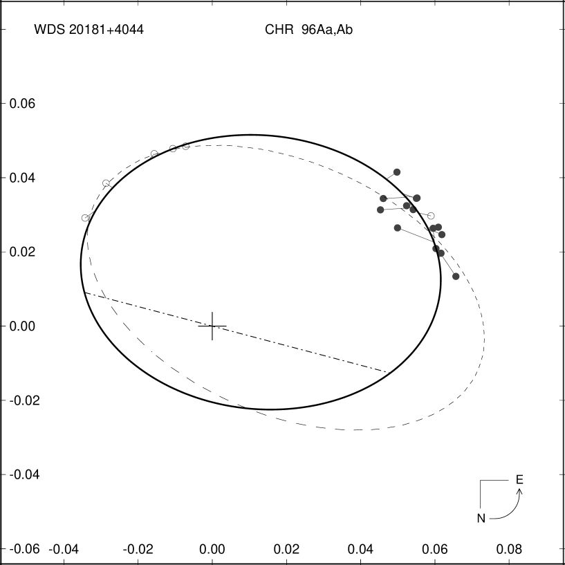
Figure 2: The astrometric orbit of the Aa,Ab pair (in units of arcsec). The dashed curve represents the first solution (Hartkopf et al. 1993) while the solid curve is the new solution (Table 2). The dot-dash line shows the line of the nodes. The filled circles represent the CHARA Array separated fringe packet results and open circles represent the speckle observations. Each measurement is connected by a line segment to the calculated position for the time of observation. Note that north is down and east to the right in this figure, and the directional arc in the lower right corner shows the counter-clockwise sense of orbital motion.

We made a new orbital solution for the wide pair using the combined set of speckle and long baseline interferometric observations. Note that we did not include the measurement from Maíz Apellániz (2010) using lucky imaging with the AstraLux instrument because of its relatively large error. All the measurements were initially assigned equal weight, but in the orbital fitting process we identified three discrepant points with large residuals that we subsequently zero-weighted in the final fit (those dates are marked in Table 1). The orbit was determined using the grid search method described by Hartkopf et al. (1989). The orbital elements are listed in Table 2 and the appearance of the visual orbit on the sky is shown in Figure 2. The original speckle data set covers about $12\%$ and the recent speckle and SFP data cover about $15\%$ of the 35 y orbit. Note that we ignored making corrections for the center of light motion of the Ab binary, because the largest astrometric shifts are expected to be small, $\approx 0.5$ mas.

3 Visual Orbit of the Close System

The interferometric fringe patterns of the close Ab1,Ab2 pair of stars overlap even with the longest baselines available at the CHARA Array, so we cannot use the separated fringe packet method to measure the relative separation. However, the interference of the two fringe patterns of the inner pair causes a modulation of their combined visibility amplitude with changes in the projected baseline separation, and we can use this modulation to estimate the binary separation projected along the baseline position angle in the sky (Hummel et al. 1998; Boden et al. 2000; Raghavan et al. 2009). The calibration of visibility is aided when the signal of a nearby star produces a separated fringe packet that can be used to calibrate the visibility of the central binary. The details of this method are outlined by O’Brien et al. (2011).

We obtained 195 observations of HD 193322 over 24 nights between 2005 and 2010 using the CHARA Array Classic beam combiner (ten Brummelaar et al. 2005). The observations were made with the near-IR $K^{\prime}$ filter and a variety of different baselines. These measurements were series of approximately 200 recorded fringe scans sampled at a frequency of 150 Hz. The scans were reduced by standard techniques (ten Brummelaar et al. 2005), and a subset of 100 scans with the best S/N were selected. We fit these scans with fringe patterns for each of the calibrator (Aa) and target (Ab) (identified according to the orbital solution from §2 and the position angle of the specific baseline; see details of the procedure in O’Brien et al. 2011). We retained only those visibility measurements for which the fractional difference between a first estimate and final mean were less than $20\%$, and these best-case values were used to form the mean visibility for each component. Note that we used the same data set as that for the wide pair (§2), but due to the stronger selection criteria not all data sets yielded useful visibility amplitudes. We next determined the ratio of the mean visibilities of the target and calibrator. This observed ratio is related to the ratio of the individual visibilities for the target and calibrator by

$$V_{\rm Ab}/V_{\rm Aa}=(F_{\rm Aa}/F_{\rm Ab})~{}V_{\rm Ab,o}/V_{\rm Aa,o}$$ (1)

where $F_{\rm Aa}/F_{\rm Ab}$ is the monochromatic flux ratio in the $K^{\prime}$-band. The angular diameter of the calibrator Aa is small enough that $V_{\rm Aa}\approx 1.0$ for our observations, but we estimated the single-star visibilities of each component based upon the projected baseline of observation and the predicted angular diameters. A value for the flux ratio of $F_{\rm Aa}/F_{\rm Ab}=10^{-0.4\triangle m_{\rm wide}}=0.92$ was adopted based upon a fit of the observed ratios and a binary model (see below), and this parameter essentially normalizes the target visibility so that the upper distribution of the visibilities has a mean of one. Note that we expected that the ratio would be $F_{\rm Aa}/F_{\rm Ab}\geq 1$ based on the speckle orbit assignments (§2), but we suspect that this difference is probably insignificant given the uncertainties in the component flux fractions. The results for the Ab pair are given in Table 3 that lists the heliocentric Julian date of observation, the corresponding orbital phase in the Ab1,Ab2 orbit (§4), the projected baseline $B_{p}$ and position angle $\psi_{p}$ of observation, the calibrated visibility and its associated error, and the observed minus calculated difference $O-C$ in visibility from the adopted model fit.

The modulation of the visibility ratio depends on the known projected baseline length and position angle and the effective wavelength of the $K^{\prime}$ system, plus the unknown projected binary separation and magnitude differences, $\triangle m_{\rm close}=-2.5\log(F_{\rm Ab2}/F_{\rm Ab1})$ and $\triangle m_{\rm wide}=-2.5\log(F_{\rm Aa}/F_{\rm Ab})$. The latter magnitude difference normalizes the visibility according to the relation given above, while the former magnitude difference sets the amplitude of the visibility modulation with baseline (Raghavan et al. 2009; O’Brien et al. 2011). Following the example of O’Brien et al. (2011), we explored the orbital parameters of the Ab1,Ab2 pair by creating a set of model visibilities for each of the observed times and baseline parameters and then forming the $\chi^{2}$ statistic for the differences between the observed and model visibilities. The solution is found by determining the orbital parameters and magnitude differences in a high resolution grid of values that minimize $\chi^{2}$. For this application of the method, we set the orbital period and epoch from the spectroscopic elements for the circular orbit of Ab1,Ab2 (§4) and then made a grid search for the best fit values of the angular semimajor axis $a$, inclination $i$, and longitude of the ascending node $\Omega$, plus the magnitude differences $\triangle m_{\rm close}$ and $\triangle m_{\rm wide}$.

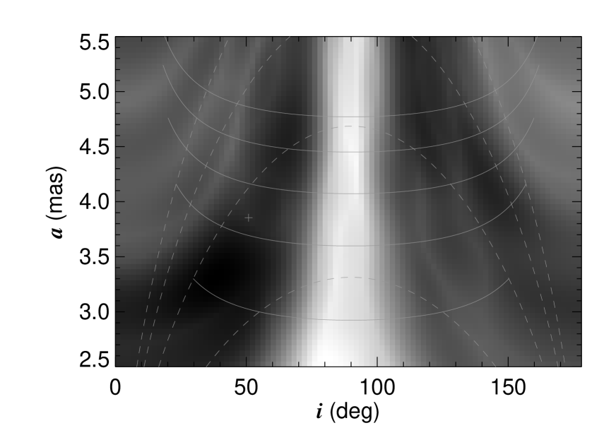
Figure 3: A gray-scale representation of the minimum $\chi^{2}$ over the full range in $\Omega$ for visibility models of the Ab1,Ab2 binary as a function of orbital inclination $i$ and angular semimajor axis $a$. Within this numerical grid of $(i,a)$, the minimum is $\chi^{2}=167$ (black) and the maximum is $\chi^{2}=529$ (white) for a sample of 195 measurements and five fitting parameters. The solid lines indicate loci of constant $M$(Ab1) (10, 20, 30, 40, and $50M_{\odot}$ from bottom to top), while the dashed lines represent loci of constant $M$(Ab2) (5, 10, 15, and $20M_{\odot}$ from bottom to top), all for an assumed distance of 741 pc. The location of the adopted solution is marked by a plus sign.

We found that the solutions always arrived at similar estimates for the magnitude differences, so we set these magnitude differences and performed a grid search over $i$ and $a$, the two parameters of physical interest. For each selection of $(i,a)$, we determined the best fit for the sky orientation parameter $\Omega$ over the full range of values in steps of $2^{\circ}$. The resulting $\chi^{2}$ estimates are plotted in a gray-scale diagram in Figure 3 in the $(i,a)$ plane for grid increments of $\triangle i=2^{\circ}$ and $\triangle a=0.05$ mas. Here intensity is scaled between the lowest (black) and highest (white) $\chi^{2}$ over the grid. If we assume a distance $d$ from the cluster fitting results of Roberts et al. (2010), then Kepler’s Third Law relates the known period $P$, the total mass, and $a$ by

$$(M({\rm Ab1})+M({\rm Ab2}))/M_{\odot}={{(ad)^{3}}\over{P^{2}}}=\left({{a}\over{1.22~{}{\rm mas}}}\right)^{3}~{}\left({d\over{741~{}{\rm pc}}}\right)^{3}.$$ (2)

Next, we can use the spectroscopic semiamplitude $K$ for component Ab1 (§4, Table 6) to derive a relation for the mass of Ab2 as a function of $i$ and $a$,

$$M({\rm Ab2})={{a^{2}}\over{P\sin i}}{{K(1-e^{2})^{1/2}}\over{29.8~{}{\rm km~{}s}^{-1}}}=0.455M_{\odot}~{}{a^{2}\over{\sin i}}~{}\left({d\over{741~{}{\rm pc}}}\right)^{2}.$$ (3)

Then we can find the mass of Ab1 from a relation for the mass ratio,

$${{M({\rm Ab1})}\over{M({\rm Ab2})}}={{29.8~{}{\rm km~{}s}^{-1}}\over{K}}{{ad\sin i}\over{P\sqrt{1-e^{2}}}}-1={{a\sin i}\over{0.819~{}{\rm mas}}}~{}\left({d\over{741~{}{\rm pc}}}\right)-1.$$ (4)

Thus, each point in the $(i,a)$ plane is associated with specific masses $M({\rm Ab1})$ and $M({\rm Ab2})$, and we can use the relations above to construct loci of constant primary and secondary mass in Figure 3 (shown by solid and dashed lines, respectively).

Inspection of Figure 3 indicates that there are two broad valleys in the $(i,a)$ plane where the fits are relatively good, one with $i<90^{\circ}$ for counterclockwise motion in the sky and another with $i>90^{\circ}$ for clockwise motion. Within these valleys there are three locations with comparable minima, but all of these are associated with extreme masses: $(i,a)=(66^{\circ},4.6~{}{\rm mas})$ ($\chi^{2}=210$) and $(i,a)=(118^{\circ},4.7~{}{\rm mas})$ ($\chi^{2}=215$) where the masses are too high and $(i,a)=(38^{\circ},3.3~{}{\rm mas})$ ($\chi^{2}=167$) where the masses are too low (see §6 below). We think that the $i<90^{\circ}$ valley probably represents the best family of solutions, since the trends in $\chi^{2}$ are more or less continuous there as expected. Between $a=2.7$ and 5.0 mas, the valley floor never rises above a reduced chi-square of $\chi^{2}_{\nu}=1.18$ (with 190 degrees of freedom, equal to 195 measurements minus five fitting parameters). Although a purely statistical assessment would restrict the solution space to the valley region around $(i,a)=(38^{\circ},3.3~{}{\rm mas})$, the fact that the reduced chi-square is close to unity along the length of the valley suggests that at this stage it is premature to rule out any of this solution space. In §6 below, we present several lines of argument that indicate that the actual solution lies in the mid-range of this valley at $a=3.85$ mas ($\chi^{2}=225$), so we will tentatively adopt this value and present the associated solution for the other orbital parameters in Table 2, column 3. The errors associated with $i$, $a$, and $\Omega$ reported in Table 2 correspond to their range over the length of the valley from $a=2.7$ to 5.0 mas. Note that because the visibility oscillation depends on the absolute value of the projected separation, there is a $180^{\circ}$ ambiguity in our derived value of $\Omega$. We found that the best fit magnitude differences are $\triangle m_{\rm close}=2.11\pm 0.06$ mag and $\triangle m_{\rm wide}=0.086\pm 0.012$ mag (Ab brighter than Aa). In order to show how well the model and observed visibilities agree, we plot the individual and calculated visibilities for this solution for each night in Figures 4 and 5, and we find that the fits are satisfactory for most of the nights.

The projection of the orbit on the sky for this solution is illustrated in Figure 6 where filled circles indicate the calculated positions at the times of observation. The distribution of the observations in orbital phase appears to constrain the minor axis of the projected ellipse better than the major axis. With the minor axis fixed, the major axis will vary with inclination as $a({\rm minor})\sim a\cos i$ or $a\propto\sec i$, and this relation approximately describes the position of the $\chi^{2}$ valley in Figure 3. The orbital orientations of the wide and close orbits appear quite different (compare Fig. 2 and Fig. 6), and the mutual inclination of the orbital planes $\phi$ is given by Fekel (1981) as

$$\cos\phi=\cos i_{\rm close}\cos i_{\rm wide}\pm\sin i_{\rm close}\sin i_{\rm wide}\cos(\Omega_{\rm close}-\Omega_{\rm wide})$$ (5)

where the second term may assume either sign because of the $180^{\circ}$ ambiguity in the determination of $\Omega_{\rm close}$. The two solutions, $\phi=38^{\circ}$ and $85^{\circ}$, indicate that the two orbits are probably far from co-planar ($\phi=0^{\circ}$).

4 Radial Velocities of Ab1

Spectroscopy potentially offers us the means to determine the masses and spectral properties of the components. However, because the stars are so close, conventional, ground-based spectroscopy records the flux of all three stars (usually plus component B at a separation of $2\farcs 7$; Turner et al. 2008), and since their orbital Doppler shifts are comparable to the line widths, the resulting line blending problem is daunting. Nevertheless, the spectral properties of the components are sufficiently different in this case that we may attempt radial velocity measurements. The appearance of the optical spectrum is dominated by a narrow-lined component that corresponds to the primary star in the close orbit, Ab1 (McKibben et al. 1998). The secondary in the close orbit, Ab2, is fainter and contributes little to the composite spectrum (§5). Furthermore, there is a very broad-lined component that appears to follow the motion of Aa in the wide orbit (§5). Because the lines of Aa are so broad and shallow, they essentially act to depress the continuum in the vicinity of the narrow lines of Ab1, and since the velocity range of Ab1 is smaller than the full width of the lines of Aa in general, the presence of the broad component has little influence on velocity measurements of Ab1 (but see a discussion of blending effects below). Here we present radial velocities for the Ab1 component and show that they represent the sum of orbital motions in both the close and wide systems.

We collected 31 new spectra for measurement from sources that are summarized in Table 4. The columns list a source number (for identification with the specific radial velocities listed in Table 5), date of observation(s), spectral range used in the measurement, the spectral resolving power, number of spectra made at that time, and the observatory, telescope aperture, and spectrograph of origin. We obtained most of these spectra in runs at the Kitt Peak National Observatory (KPNO) 0.9 m coudé feed and 4 m Mayall Telescopes, the 3.6 m Canada-France-Hawaii Telescope, the 2.5 m Nordic Optical Telescope, the Lowell Observatory 1.8 m Perkins Telescope, and the Herzberg Institute of Astrophysics, Dominion Astrophysical Observatory 1.8 m Plaskett Telescope. These were augmented with publicly available spectra from the archives of the University of Toledo Ritter Observatory 1.0 m telescope (Morrison et al. 1997), the Observatoire de Haute-Provence 1.9 m telescope and ELODIE spectrograph (Moultaka et al. 2004), and the Indo-U.S. Library of Coudé Feed Stellar Spectra (Valdes et al. 2004; made with the KPNO 0.9 m coudé feed telescope). All these spectra were reduced by standard techniques and transformed to a continuum normalized flux representation on a heliocentric, $\log$ wavelength grid. Atmospheric telluric lines were removed from the red spectra by division with a pure atmospheric spectrum. This was done by creating a library of spectra from each run of a rapidly rotating A-star (usually $\zeta$ Aql), removing the broad stellar features from these, and then dividing each target spectrum by the modified atmospheric spectrum that most closely matched the target spectrum in a selected region dominated by atmospheric absorptions.

The spectra form a diverse collection with a wide range in resolving power and wavelength coverage. In order to measure radial velocities in a consistent way, we cross-correlated each of the spectra with a standard, model spectrum (rest frame) from the grid of synthetic spectra from Lanz & Hubeny (2003). From an initial inspection of the observations, we selected a model with Galactic abundances, effective temperature $T_{\rm eff}=34.8$ kK, gravity $\log g=4.0$, projected rotational velocity $V\sin i=50$ km s^-1, a wavelength dependent limb darkening coefficient from Wade & Rucinski (1985), and an instrumental broadening appropriate for the specific observed spectrum. The cross-correlations were generally made over the wavelength range given in Table 4, although in some cases regions with strong interstellar features were omitted. The resulting cross-correlation functions were always single-peaked, and we measured the radial velocity and its associated error using the method of Zucker (2003). The results are presented in Table 5 that lists the heliocentric Julian date of mid-exposure, the corresponding orbital phases in the close and wide systems (see below), the measured radial velocity and its associated error, a correction term for line blending effects, the observed minus calculated velocity residual from the fit (see below), and the observation source number from Table 4. Note that for completeness we have included in Table 5 velocities published earlier by McKibben et al. (1998; indicated by a 0 in the final column).

Although the line blending effects from the spectral components of the other stars are generally small, they tend to bias the measurements towards the systemic velocity and lead to a slight underestimate of the orbital semiamplitude. The radial velocity offset caused by line blending will depend on the character and velocity shift of each component, the spectral features measured, and the spectral resolution of the observation. In order to make a simple correction for line blending effects we adopted the following procedure for each observation. We first determined model synthetic spectra for each stellar component (§5) for the spectral range and instrumental broadening of the observation. The models for components Aa, Ab2, and B were co-added according to the adopted fluxes and to the Doppler shifts for the time of observation. Then we formed a series of model spectra by adding in component Ab1 for a grid of assigned velocity offsets, and we measured the radial velocity in these composite spectra using the same cross-correlation method applied to the observations. This led to a relation between the actual and measured radial velocity for each observation, and we interpolated within this relation at the observed radial velocity to determine the offset correction for blending $\Delta V_{r}({\rm blend})=V_{r}({\rm actual})-V_{r}({\rm measured})$, which is given in Table 5, column 6. The average of the absolute value of the offset correction for blending is small, 2.3 km s^-1, but the individual offset corrections are larger for the lower resolution spectra where line blending is more severe.

The velocities of component Ab1 depend on its orbital motion in the close binary plus the motion of the Ab1,Ab2 center of mass in the orbit of the Aa,Ab system. Our first solutions for the orbital motion of the close binary clearly showed long term variations in the residuals that followed the motion predicted for Ab in the wide orbit. Thus, we fit the observed radial velocity variations as the sum of motions in the close and wide binaries. This was done iteratively using the orbital fitting program of Morbey & Brosterhus (1974). We first made a general fit of the velocities for the close system, and then we made a constrained fit of the velocity residuals, by fixing $P$, $e$ and $\omega$ from the visual orbit of Aa,Ab to find the semiamplitude $K$ and epoch of periastron $T$ for the wide system. The resulting solution of the long period orbit was then used to correct the observed velocities for motion in the wide orbit, and a new solution was found for the close orbit. This procedure quickly converged to yield the orbital elements given in Table 6. Note that we assigned each measurement a weight proportional to $\sigma(V_{r})^{-2}$ in making the fits, and we zero-weighted four measurements that had unusually large residuals from the final fit (dates indicated in Table 5 and shown as open circles in Fig. 7). Table 6 lists the solutions both with and without application of the offset correction for line blending, and they are generally very similar except for the slightly larger semiamplitude $K$ that results when accounting for line blending. Since the line blending problem is significant, we adopt the corrected velocity solutions that are illustrated in Figure 7 (close orbit) and Figure 8 (wide orbit) and that form the basis for the residuals $O-C$ given in Table 5, column 7. We found that the eccentricity associated with the close orbit is not statistically different from zero according to the criterion of Lucy & Sweeney (1971), so we present circular elements in Table 6 (where the epoch $T$ is defined as the time of maximum radial velocity or, equivalently, the time of crossing the ascending node). The long orbital period of the wide system, $P=35$ y, places HD 193322 among the top $1\%$ of known spectroscopic binaries with very long periods (Pourbaix et al. 2004).

5 Spectroscopic Properties

The two brightest components of HD 193322, Aa and Ab1, have very broad and very narrow spectral lines, respectively, and indeed it is these properties that can help us distinguish their different orbital motions. We show in Figure 9 CFHT spectra of the He I $\lambda 5876$ profile from 1986 and 2008. During this interval, the broad component moved slightly redward as expected for the anti-phase velocity curve of Aa between wide orbit phases 0.82 and 0.44 (Fig. 8). We collected all the available red spectra that recorded He I $\lambda 5876$, and we formed an average spectrum for each run in order to increase the S/N of the spectra at each epoch. We then formed model spectra for each of Aa and Ab1 from the grid of Lanz & Hubeny (2003) using projected rotational velocities and model parameters optimized to match the composite profile (see below). These model profiles were fit to the observations using a non-linear, least-squares procedure to derive the radial velocities of Aa and Ab1 at these epochs. The derived Ab1 velocities are identical within errors to the corresponding measurements given in Table 5, and the velocities for Aa are listed in Table 7. The errors associated with the velocities of Aa are large, $\pm 20$ km s^-1, because this component is so broad and shallow and because the shape of the red wing is sensitive to the details of the removal of the telluric features found there. Given these larger errors and the relatively small number of measurements, we made a constrained fit of the orbital radial velocity curve of Aa by setting all the parameters from the solution for Ab (Table 6) with the exception of the systemic velocity $\gamma$ and semiamplitude $K$, and by assigning a weight to each observation proportional to the product of the spectral resolving power and the net S/N ratio in the adjoining continuum (column 5 of Table 7). The fit (illustrated in Fig. 8) yielded $\gamma=-12\pm 8$ km s^-1 and $K=21\pm 16$ km s^-1, with a residual rms $=21$ km s^-1. These measurements are consistent with the expected Doppler shifts and masses for the Aa,Ab system (§6).

We estimated the spectroscopic parameters for the components by first reconstructing their spectra using the orbital velocity curves and a Doppler tomography algorithm (Bagnuolo et al. 1994) and then comparing the reconstructions with models from the grids of Lanz & Hubeny (2003, 2007). We selected nine spectra from our observations that recorded the blue portion of the spectrum with a resolving power greater than 10000 and that covered the extremes of motion in the wide and close systems (samples 10, 12, 14, 15, and 16 from Table 4). We began by running the tomography algorithm for only two components, Aa and Ab1, however, we found that the subsequent reconstructed spectrum for Aa had a composite appearance with both broad and narrow components, unlike our expectation from the He I $\lambda 5876$ profiles (Fig. 9). We think that this is due to flux contamination in our blue spectra from the nearby B component (B1.5 V; $V\sin i\approx 100$ km s^-1; see McKibben et al. 1998, Fig. 2, and Roberts et al. 2010, Fig. 1). Although component B may be a spectroscopic binary with a low semiamplitude (McKibben et al. 1998), we simply assumed that it was stationary and contributed $11\%$ of the total flux (Roberts et al. 2010) in the next iteration of tomographic reconstruction. The power of the tomography algorithm to derive reliable and high quality reconstructed spectra increases with the number of spectra and with the orbital velocity range and flux contribution of the components. Unfortunately, in the case of our blue spectra of HD 193322, these criteria are really only met for component Ab1. The velocity range of Aa, for example, is so small relative to its characteristic line width that the algorithm may incorrectly assign line flux between the reconstruction of Aa and the stationary component B. We dealt with this problem by starting the initial guess for components Aa, Ab2, and B with model spectra rather than assuming a flat continuum spectrum (as done for Ab1). Although the resulting solutions are guided by our assumptions, they do at least show that the observed spectra are consistent with these assumptions since otherwise the reconstructed spectra would converge to an appearance different from the initial model guesses.

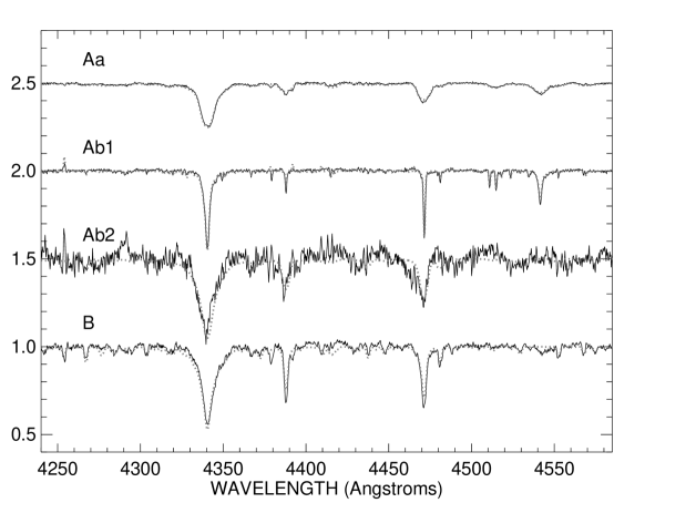
Figure 10: Example tomographic reconstructions of the blue spectra of the components of HD 193322. The solid lines show the Doppler tomography spectra while the dotted gray lines show superimposed model spectra. The spectra are offset by steps of $50\%$ of the continuum for clarity.

We show the results of the full, four-component, tomographic reconstructions in Figure 10. These representative solutions were made using the orbital solutions from Table 6, adopting a mass ratio of $M({\rm Ab2})/M({\rm Ab1})=0.37$ (§6) and the flux ratios given in Table 8. These flux ratios were calculated from the $K^{\prime}$-band $\triangle m_{\rm close}$ and $\triangle m_{\rm wide}$ results (§3) assuming that these hot stars all contribute by the same proportions in the $B$-band. The spectroscopic parameters were determined by finding the Lanz & Hubeny (2003, 2007) model that best matched the absorption line ratios and H$\gamma$ Stark broadening (dependent on $T_{\rm eff}$ and $\log g$) and with a $V\sin i$ value adjusted to fit the widths of the absorption lines other than H$\gamma$. The results are listed in columns 2 and 3 of Table 8 for Aa and Ab1, respectively, and we estimate that the associated errors are $\triangle T_{\rm eff}=\pm 1$ kK, $\triangle\log g=\pm 0.5$, and $\triangle V\sin i=\pm 40$ and $\pm 10$ km s^-1 for Aa and Ab1, respectively. These parameters suggest spectral classifications of O9 Vnn and O8.5 III for Aa and Ab1, respectively, based upon the calibration of Martins et al. (2005). The “nn” suffix for the former classification indicates very broad lines. The relatively good agreement between the observed and model line depths indicates that the flux ratios from interferometry (§3) are fully consistent with the derived strengths of the spectroscopic features. The parameters in Table 8 for component B were taken from the work of Roberts et al. (2010), and the predicted model spectrum agrees well with the narrow, stationary spectral component from the tomographic reconstruction. The results for the faintest component, Ab2, are poorly constrained because this star contributes such a small fraction of the total flux, but its spectrum suggests an early-B, dwarf classification. We used the flux ratio between Ab2 and B and the temperature of B and the theoretical main sequence $(T_{\rm eff},M_{V})$ adopted by Roberts et al. (2010) in order to estimate the effective temperature of Ab2, assuming it is a main sequence star. The H$\gamma$ $\lambda 4340$ line is the only strong feature in the reconstructed spectrum of Ab2, and the relative weakness of the He I $\lambda\lambda 4387,4471$ lines suggest that Ab2 may also be a rapid rotator with broad and shallow lines. Note that the $V\sin i$ estimate for Ab2 in Table 8 is only approximate and may be subject to significant revision.

6 Discussion

One of the primary goals of this study was to determine the masses of the component stars. Since most of our results are preliminary, we cannot yet derive accurate masses, but the observational work does demonstrate the potential for improvement with further interferometric and spectroscopic observations. The mass sums for the wide and close systems can be determined from the angular semimajor axes and orbital periods (Table 2) and the distance $d=741\pm 36$ pc for Collinder 419 (Roberts et al. 2010). The mass sums (eq. 2) are $(M({\rm Aa})+M({\rm Ab1})+M({\rm Ab2}))/M_{\odot}=(53.2\pm 11.5)~{}(d/[741~{}{\rm pc}])^{3}$ for the wide system and $(M({\rm Ab1})+M({\rm Ab2}))/M_{\odot}=35.6~{}(a/[4.0~{}{\rm mas}])^{3}~{}(d/[741~{}{\rm pc}])^{3}$ for the close system (where $a$ is the angular semimajor axis of Ab1,Ab2).

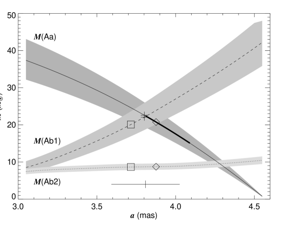
Figure 11: A diagram of the mass solutions for components Aa (solid line), Ab1 (dashed line), and Ab2 (dotted line) as a function of $a$, the angular semimajor axis of the Ab1,Ab2 system. The shaded region surrounding each line corresponds to the $\pm 1\sigma$ error range in distance. The thick portion of the Aa line shows the section that intersects with the $\pm 1\sigma$ error range for the mass of Aa as determined from the visual wide orbit, assumed distance, and the Ab1,Ab2 center-of-mass radial velocity curve (Fig. 8). The various symbols indicate the positions where the mass ratios match those of main sequence stars with the observed flux ratios (squares for $F$(Ab2)/$F$(Ab1), crosses for $F$(Ab1)/$F$(Aa), and diamonds for $F$(Ab2)/$F$(Aa)). The tick mark at bottom indicates those masses for which the sum of the corresponding fluxes of main sequence stars attains a minimum, the situation most consistent with the estimated total absolute magnitude, and the horizontal line segment shows the range over which the absolute magnitude is within 0.1 mag of the faint limit.

To obtain the individual masses, we need to explore the solution space from the interferometric observations of the close binary (Fig. 3) and from the spectroscopic orbit of Ab1 (Table 6). In particular, we can use the location of the $\chi^{2}$ valley in the $(i,a)$ plane of Figure 3 to derive a family of solutions based solely upon $a$ (since $i=i(a)$ from Fig. 3). We show the derived individual masses as a function of $a$ in Figure 11. The mass of Aa is set from the difference of the total mass of Aa,Ab and the mass of Ab1,Ab2 (from $a$ and eq. 2); the mass of Ab2 is from eq. 3 (from $a$, $K$(Ab1), and the $i=i(a)$ relation in Fig. 3); and the mass of Ab1 is from the difference $M({\rm Ab1,Ab2})-M({\rm Ab2})$. These are all plotted in Figure 11 surrounded by a gray zone corresponding to the acceptable range in cluster distance. We see that there is a strict upper limit of $a<4.57$ mas required to keep $M({\rm Aa})>0$. Furthermore, we also see that while the masses of Aa and Ab1 cover a significant range, the mass of Ab2 changes little over the range in $a$. This is also shown in Figure 3, where the location of the $\chi^{2}$ valley is close to a contour of constant $M({\rm Ab2})$.

Another constraint on the mass of Aa can be formed independent of the details of the Ab1,Ab2 orbit by applying eq. 3 to the wide orbit. We take $a$, $P$, $e$, and $i$ from the visual orbit of the wide system (Table 2) and combine these with the orbital semiamplitude $K({\rm Ab})$ from spectroscopy (Table 6) to obtain $M({\rm Aa})/M_{\odot}=(18.7\pm 3.7)(d/[741~{}{\rm pc}])^{2}$. The $\pm 1\sigma$ region from this relation is plotted as the thick line segment for $M({\rm Aa})$ in Figure 11, and it corresponds to a range in semimajor axis of $a=3.96\pm 0.14$ mas.

It is reasonable to assume that all three stars are main sequence objects given the position of the Aa,Ab system in the color-magnitude diagram (Roberts et al. 2010). The $K$-band fluxes of massive main sequence stars scale with mass $M$ as $F\propto M^{2.30}$ for stars in this mass range according to the models of Marigo et al. (2008), so we can use this relation to predict the flux ratio between any pair of stars according to the mass relations shown in Figure 11. The positions where the model flux ratios match the observed ones (Table 8) are indicated by pairs of symbols in Figure 11. These flux ratio relations indicate a semimajor axis range of $a=3.80\pm 0.08$ mas.

A final constraint can be set from the overall fluxes and absolute magnitude of the combined system. Ten Brummelaar et al. (2000) estimate that the apparent $V$-band magnitude of Aa,Ab is $V=5.96\pm 0.02$ mag, and using the distance and extinction for the star from Roberts et al. (2010), we estimate that the absolute magnitude is $M_{V}=-4.35\pm 0.12$ mag. The individual absolute magnitudes of the components are given in Table 8. We can apply the mass – absolute magnitude relation $(M,M_{V})$ for the main sequence from the models of Marigo et al. (2008) to obtain a prediction for the total absolute magnitude for each of the mass combinations shown in Figure 11. The best match occurs for the masses obtained at $a=3.81$ mas, approximately where Aa and Ab1 have equal masses. For those masses the predicted absolute magnitude is $M_{V}=-5.12$, which is significantly brighter than the estimate above from observations. The models predict even brighter fluxes if either of Aa or Ab1 are more massive, and the horizontal line at the bottom of Figure 11 shows the range in $a$ where the combined magnitude is within 0.1 mag of the faint limit.

The average estimate for the semimajor axis from the above three constraints is $a=3.85\pm 0.09$ mas, and we adopt the associated mass solution as best representing the current observational data. The masses and other properties summarized in Table 8 are generally in agreement with expectations for hot, main sequence stars (Martins et al. 2005). However, there remain a number of significant discrepancies that deserve further investigation. The mass of component Ab1 is similar to that expected for an O8.5 III star ($\approx 24M_{\odot}$; Martins et al. 2005), but the star’s absolute magnitude is about 1.8 mag fainter than typical for such stars. This discrepancy hints that Ab1 may be a dwarf rather than a giant star. The overall faintness of the system compared with expectations for the stars’ masses may indicate that the distance estimate needs to be revised downward (leading to lower masses) and/or the extinction estimate revised upwards. There also remains some confusion about which of Aa or Ab1,Ab2 is brighter. As we noted in §3, the visibility analysis indicates that $\triangle m_{\rm wide}=m({\rm Aa})-m({\rm Ab})=0.086\pm 0.012$ mag (Ab brighter than Aa), which agrees within errors with high angular resolution measurements using the AstraLux camera by Maíz Apellániz (2010), $m({\rm Aa})-m({\rm Ab})=0.04\pm 0.19$ mag. Although these results indicate that Ab is somewhat brighter than Aa, we refrain from re-designating the identities of the components to avoid confusion with published results.

We expect that these lingering problems will be resolved with future interferometric observations that will better sample the orbital phases of the close pair near the nodal crossings and will lead to improved constraints on the angular semimajor axis $a$. In addition, we clearly need to continue the long term high resolution work on the wide orbit to cover the missing orbital phases (Fig. 2). We plan to obtain these measurements through continuing observations of this system using the CHARA Array interferometer. Additional high S/N and high resolution spectroscopy holds the promise to deliver better orbital constraints on Aa and Ab2 that would then allow us to estimate the masses without relying on the distance of the cluster. Indeed, reliable orbital elements would render it possible to set an independent estimate of the cluster distance. We anticipate expanding the spectroscopic coverage over the next decade.

We close with some speculative remarks about the angular momentum distribution of the stars of HD 193322. It is remarkable that this system contains both a very rapidly rotating star (Aa) and a very slowly rotating star (Ab1). It is possible that Ab1 has a rotational axis with a low inclination, so that its equatorial rotational velocity is close to typical values. However, the very large line broadening of Aa places it among the most rapidly rotating O-type stars known (Penny 1996). It is possible that the angular momentum of the natal cloud led directly to rapid rotation in the case of Aa and to the formation of a binary in the case of Ab. Alternatively, there may have been some very close gravitational encounters in the early life of the system. In some circumstances, a close encounter between a binary and a third interloper can lead to a merger of two of the components and ejection of the third (Gaburov et al. 2010). It is possible that the rapid rotator Aa is such a merger product and that the runaway star 68 Cygni was the object ejected from the system (Schilbach & Röser 2008). If so, then the orbital and spin properties of the stars of HD 193322 offer key evidence about the early dynamical processes in this cluster.

Table 1: Astrometric Measurements of Aa,Ab

Date	$\theta$	$\rho$	Data
(BY)	(deg)	(arcsec)	Type	Reference
1985.5177	188.4	0.0490	Speckle	McAlister et al. (1993)
1985.8396	192.5	0.0490	Speckle	McAlister et al. (1993)
1986.8884	198.6	0.0490	Speckle	McAlister et al. (1993)
1988.6630	216.6	0.0480	Speckle	McAlister et al. (1993)
1989.7061	229.6	0.0450	Speckle	McAlister et al. (1993)
2005.6054	109.1	0.0638	OLBI/SFP	This paper
2005.7350	107.7	0.0647	OLBI/SFP	This paper
2005.8652	100.4	0.0860	Speckle	Mason et al. (2009)
2006.4324	100.1	0.0409	OLBI/SFP	This paper
2006.4897	101.5	0.0670	OLBI/SFP	This paper
2006.5881	113.9	0.0651	OLBI/SFP	This paper
2006.6758	118.0	0.0565	OLBI/SFP	This paper
2007.4729	111.7	0.0666	OLBI/SFP	This paper
2007.5098	113.6	0.0665	OLBI/SFP	This paper
2007.6042	100.9	0.0670	Speckle	Mason et al. (2009)
2008.4508	116.8	0.0660	Speckle	Mason et al. (2009)
2008.6198	121.8	0.0616	OLBI/SFP	This paper
2008.8028	124.7	0.0551	OLBI/SFP	This paper
2009.4178	120.1	0.0626	OLBI/SFP	This paper
2009.5017	126.7	0.0575	OLBI/SFP	This paper
2009.6146	122.0	0.0651	OLBI/SFP	This paper
2009.7776	122.0	0.0649	OLBI/SFP	This paper
2010.8753	129.8	0.0648	OLBI/SFP	This paper

Table 2: Visual Orbital Elements

Element	Aa,Ab Orbit	Ab1,Ab2 Orbit
$P$ (y)	$35.20\pm 1.45$	0.85533
$P$ (d)	$12855\pm 528$	312.40
$T$ (BY)	$1994.84\pm 1.69$	1996.109
$T$ (HJD–2,400,000)	$49662\pm 616$	50123.5
$a$ (mas)	$54.5\pm 3.7$	$3.9^{+1.1}_{-1.2}$
$i$ (deg)	$46.2\pm 6.9$	$51^{+17}_{-51}$
$\Omega$ (deg)	$255.2\pm 15.0$	$25^{+3}_{-35}$
$e$	$0.489\pm 0.081$	0
$\omega$ (deg)	$70.4\pm 7.5$	180

Table 3: Visibility Measurements of Ab1,Ab2

Date	$\phi$	$B_{p}$	$\psi_{p}$
(HJD$-$2,400,000)	(close)	(m)	(deg)	$V$	$\triangle V$	$O-C$
53591.721	0.102	098.8	118.8	1.035	0.175	+0.045
53591.756	0.102	104.3	109.0	0.968	0.147	$-$0.020
53591.785	0.102	107.0	101.9	0.912	0.125	$-$0.024
53591.818	0.102	107.9	093.9	0.812	0.108	$-$0.039
53591.842	0.102	106.9	088.5	0.697	0.095	$-$0.104
53591.855	0.102	105.7	085.3	0.740	0.097	$-$0.038
53591.888	0.102	101.1	077.2	0.679	0.093	$-$0.073
53591.912	0.102	096.2	070.6	0.667	0.088	$-$0.084
53638.741	0.252	170.6	324.4	0.893	0.242	+0.137
53638.747	0.252	169.8	323.5	0.702	0.119	$-$0.057
53638.753	0.252	168.9	322.4	0.853	0.153	+0.090
53638.757	0.252	168.2	321.7	0.797	0.150	+0.031
53638.765	0.252	166.8	320.4	0.724	0.129	$-$0.047
53638.769	0.252	166.1	319.8	0.834	0.160	+0.061
53638.775	0.252	164.9	318.9	0.802	0.170	+0.025
53638.779	0.252	164.0	318.3	0.778	0.173	$-$0.001
53638.782	0.252	163.3	317.8	0.940	0.169	+0.159
53638.787	0.252	162.2	317.1	1.023	0.145	+0.240
53638.791	0.252	161.2	316.5	0.920	0.174	+0.135
53638.794	0.252	160.6	316.1	0.780	0.162	$-$0.007
53638.798	0.252	159.4	315.4	0.884	0.166	+0.096
53638.804	0.252	158.0	314.7	0.817	0.174	+0.027
53638.809	0.252	156.5	314.0	0.938	0.155	+0.148
53638.813	0.253	155.4	313.5	0.931	0.218	+0.140
53639.696	0.255	107.6	091.8	0.831	0.118	+0.057
53639.701	0.255	107.4	090.6	0.778	0.119	+0.005
53639.705	0.255	107.2	089.6	0.817	0.120	+0.045
53639.713	0.255	106.7	087.8	0.901	0.140	+0.130
53639.717	0.255	106.3	086.8	0.775	0.111	+0.005
53639.723	0.255	105.7	085.3	0.765	0.118	$-$0.002
53639.729	0.255	105.0	083.8	0.594	0.087	$-$0.171
53639.732	0.255	104.6	083.1	0.722	0.122	$-$0.041
53639.736	0.255	104.2	082.2	0.732	0.106	$-$0.031
53639.739	0.255	103.8	081.5	0.829	0.159	+0.068
53639.743	0.255	103.2	080.5	0.785	0.116	+0.026
53639.746	0.255	102.6	079.6	0.888	0.173	+0.130
53639.750	0.256	102.0	078.6	0.834	0.145	+0.078
53639.754	0.256	101.4	077.6	0.638	0.097	$-$0.117
53639.757	0.256	100.9	076.9	0.734	0.110	$-$0.020
53639.767	0.256	099.0	074.3	0.792	0.148	+0.040
53639.769	0.256	098.5	073.6	0.729	0.128	$-$0.022
53639.774	0.256	097.5	072.3	0.848	0.198	+0.098
53639.778	0.256	096.7	071.3	0.611	0.116	$-$0.139
53639.781	0.256	096.0	070.3	0.666	0.113	$-$0.085
53639.785	0.256	095.1	069.2	0.832	0.170	+0.081
53639.788	0.256	094.4	068.3	0.917	0.147	+0.166
53639.793	0.256	093.3	066.9	0.938	0.198	+0.185
53639.797	0.256	092.3	065.7	1.270	0.244	+0.515
53639.800	0.256	091.7	064.9	1.379	0.290	+0.622
53639.808	0.256	089.7	062.4	1.003	0.240	+0.240
53639.812	0.256	088.6	061.1	0.776	0.159	+0.008
53639.816	0.256	087.4	059.5	0.922	0.221	+0.148
53639.822	0.256	086.0	057.7	1.040	0.222	+0.258
53893.877	0.069	315.5	039.3	1.154	0.163	+0.357
53893.886	0.069	318.1	037.7	0.989	0.144	+0.209
53893.889	0.069	319.0	037.1	0.893	0.127	+0.117
53893.898	0.069	321.1	035.5	0.839	0.130	+0.068
53893.912	0.069	323.8	033.0	1.062	0.146	+0.287
53893.915	0.069	324.3	032.4	1.088	0.154	+0.309
53893.923	0.069	325.6	030.8	1.180	0.160	+0.392
53893.926	0.069	325.9	030.3	1.031	0.136	+0.240
53893.935	0.069	327.0	028.6	0.931	0.130	+0.128
53914.806	0.136	093.0	128.0	1.021	0.134	+0.024
53914.815	0.136	094.8	125.1	1.044	0.160	+0.045
53914.824	0.136	096.7	122.1	1.072	0.141	+0.075
53914.829	0.136	097.6	120.7	1.029	0.137	+0.036
53914.837	0.136	099.2	118.1	1.044	0.144	+0.059
53914.842	0.136	099.9	117.0	0.940	0.125	$-$0.038
53914.850	0.136	101.4	114.5	0.925	0.125	$-$0.039
53914.859	0.136	102.7	112.2	0.937	0.123	$-$0.009
53914.865	0.136	103.6	110.4	0.872	0.124	$-$0.059
53950.685	0.251	088.2	136.2	0.896	0.123	+0.077
53950.695	0.251	090.2	132.7	0.704	0.093	$-$0.095
53950.701	0.251	091.5	130.5	0.773	0.103	$-$0.015
53950.708	0.251	092.9	128.3	0.770	0.102	$-$0.007
53950.716	0.251	094.5	125.7	0.692	0.090	$-$0.075
53950.724	0.251	096.1	123.1	0.759	0.100	$-$0.000
53950.730	0.251	097.3	121.1	0.687	0.091	$-$0.067
53950.736	0.251	098.5	119.3	0.667	0.089	$-$0.085
53950.744	0.251	100.0	116.9	0.733	0.096	$-$0.017
53950.755	0.251	101.7	113.9	0.760	0.101	+0.010
53950.764	0.251	103.0	111.6	0.678	0.090	$-$0.074
53950.781	0.251	105.2	107.1	0.797	0.105	+0.039
53950.788	0.251	105.9	105.3	0.778	0.104	+0.017
53950.803	0.251	107.1	101.7	0.849	0.122	+0.082
53950.814	0.251	107.7	098.9	0.826	0.121	+0.055
53950.819	0.251	107.8	097.9	0.729	0.105	$-$0.043
53950.830	0.251	107.9	095.3	0.719	0.103	$-$0.054
53950.838	0.251	107.8	093.2	0.774	0.103	$-$0.000
53950.843	0.251	107.7	092.2	0.829	0.114	+0.055
53950.852	0.251	107.3	090.1	0.808	0.119	+0.035
53950.861	0.251	106.7	088.0	0.720	0.096	$-$0.051
53950.866	0.251	106.2	086.6	0.839	0.114	+0.069
53950.875	0.251	105.3	084.5	0.785	0.110	+0.018
53950.888	0.251	103.8	081.5	0.751	0.104	$-$0.012
53950.900	0.251	101.9	078.4	0.836	0.112	+0.079
53950.904	0.251	101.3	077.5	0.708	0.096	$-$0.048
53982.762	0.353	174.5	331.3	1.133	0.154	+0.199
53982.769	0.353	174.0	330.0	1.068	0.147	+0.135
53982.777	0.354	173.2	328.4	1.070	0.142	+0.137
53982.782	0.354	172.7	327.4	1.088	0.141	+0.156
53982.791	0.354	171.8	326.0	1.017	0.136	+0.083
53982.797	0.354	171.0	324.9	1.017	0.135	+0.081
53982.805	0.354	169.8	323.5	1.008	0.135	+0.069
53982.814	0.354	168.5	322.1	0.975	0.135	+0.031
53982.818	0.354	167.8	321.3	1.018	0.136	+0.072
53982.827	0.354	166.1	319.9	1.053	0.138	+0.100
53982.849	0.354	161.4	316.6	0.677	0.110	$-$0.292
53982.854	0.354	160.2	315.9	1.053	0.138	+0.080
53982.863	0.354	157.7	314.6	1.040	0.139	+0.060
54273.899	0.285	105.6	106.2	0.747	0.112	$-$0.032
54273.910	0.285	106.6	103.5	0.702	0.103	$-$0.079
54273.914	0.285	106.9	102.3	0.795	0.110	+0.014
54273.930	0.286	107.7	098.5	0.798	0.106	+0.018
54273.938	0.286	107.9	096.6	0.789	0.104	+0.011
54273.948	0.286	107.9	094.4	0.789	0.105	+0.013
54273.958	0.286	107.7	091.9	0.879	0.114	+0.107
54273.963	0.286	107.5	090.8	0.794	0.103	+0.024
54273.979	0.286	106.3	086.9	0.847	0.109	+0.085
54273.987	0.286	105.6	085.1	0.785	0.101	+0.027
54273.997	0.286	104.4	082.7	0.719	0.093	$-$0.035
54285.938	0.324	247.9	008.0	0.761	0.169	$-$0.130
54288.939	0.334	247.9	006.0	1.072	0.164	+0.090
54288.986	0.334	248.0	355.4	0.860	0.141	$-$0.080
54289.971	0.337	248.0	358.2	0.755	0.115	$-$0.195
54289.975	0.337	248.0	357.3	0.700	0.272	$-$0.240
54318.890	0.429	330.7	002.5	1.094	0.144	+0.316
54412.690	0.730	089.5	062.2	1.096	0.226	+0.345
54412.715	0.730	082.9	053.5	0.839	0.141	+0.073
54412.727	0.730	079.9	049.1	0.716	0.115	$-$0.065
54412.739	0.730	076.8	044.2	0.801	0.131	$-$0.000
54606.005	0.348	278.4	143.2	0.732	0.191	$-$0.218
54657.944	0.515	267.3	127.0	0.731	0.156	$-$0.092
54657.959	0.515	262.1	124.1	0.986	0.191	+0.074
54657.968	0.515	258.6	122.5	1.115	0.181	+0.161
54692.830	0.626	272.2	130.7	0.684	0.096	$-$0.147
54692.837	0.626	270.6	129.3	0.727	0.096	$-$0.143
54692.889	0.627	330.7	177.4	1.008	0.146	+0.033
54692.897	0.627	330.7	175.6	1.068	0.144	+0.099
54692.905	0.627	330.7	173.9	0.761	0.112	$-$0.196
54692.912	0.627	330.7	172.0	0.702	0.127	$-$0.232
54692.946	0.627	330.4	164.3	0.702	0.196	$-$0.087
54692.960	0.627	330.1	161.2	0.580	0.128	$-$0.174
54759.629	0.840	275.2	134.0	0.983	0.168	+0.063
54759.667	0.840	330.7	186.2	0.997	0.175	+0.193
54759.677	0.840	330.7	183.9	1.271	0.183	+0.503
54759.687	0.840	330.7	181.6	1.092	0.203	+0.340
54759.696	0.840	330.7	179.5	1.380	0.215	+0.623
54759.728	0.841	238.0	115.8	1.088	0.206	+0.332
54759.765	0.841	330.3	163.6	0.809	0.133	$-$0.151
54759.790	0.841	329.5	158.0	0.816	0.133	$-$0.160
54983.996	0.558	277.2	137.8	0.640	0.091	$-$0.172
54984.002	0.558	276.7	136.6	0.766	0.100	$-$0.076
54984.865	0.561	262.4	100.2	1.204	0.160	+0.239
54984.871	0.561	267.1	098.6	1.186	0.156	+0.260
54984.876	0.561	270.9	097.3	1.175	0.163	+0.288
54984.882	0.561	274.5	096.1	0.926	0.124	+0.079
54984.887	0.561	278.1	094.8	0.926	0.121	+0.122
54984.892	0.561	281.4	093.6	0.785	0.105	+0.013
54984.904	0.561	276.2	159.5	1.145	0.151	+0.179
54984.907	0.561	276.5	158.2	1.150	0.151	+0.194
54984.916	0.561	276.9	156.2	1.012	0.139	+0.077
54984.921	0.561	277.2	154.9	1.078	0.151	+0.161
55014.938	0.657	330.5	193.5	1.151	0.152	+0.188
55014.943	0.657	330.6	192.3	0.988	0.131	+0.032
55014.948	0.657	330.6	191.3	1.023	0.137	+0.076
55014.952	0.657	330.6	190.1	0.986	0.133	+0.051
55014.957	0.658	330.6	188.9	1.009	0.145	+0.088
55014.963	0.658	330.7	187.4	0.819	0.144	$-$0.081
55014.969	0.658	330.7	186.0	0.909	0.203	+0.030
55014.975	0.658	330.7	184.6	0.790	0.106	$-$0.066
55014.981	0.658	330.7	183.4	0.729	0.102	$-$0.106
55014.986	0.658	330.7	182.0	0.728	0.099	$-$0.084
55014.992	0.658	330.7	181.0	0.765	0.103	$-$0.031
55054.879	0.785	248.0	178.1	1.020	0.149	+0.274
55054.883	0.785	248.0	177.0	1.245	0.182	+0.497
55054.888	0.785	248.0	176.0	1.041	0.169	+0.289
55054.892	0.785	247.9	174.9	0.846	0.125	+0.086
55055.855	0.788	248.0	182.7	1.144	0.173	+0.386
55055.859	0.788	248.0	181.9	1.075	0.167	+0.322
55055.865	0.788	248.0	180.9	1.021	0.177	+0.274
55055.895	0.789	247.9	174.0	0.603	0.116	$-$0.190
55055.897	0.789	247.9	173.1	0.630	0.112	$-$0.175
55055.903	0.789	247.9	172.0	0.776	0.126	$-$0.048
55056.827	0.792	247.8	188.6	1.337	0.189	+0.521
55056.835	0.792	247.9	186.9	1.172	0.281	+0.384
55056.841	0.792	247.9	185.4	1.563	0.316	+0.794
55056.847	0.792	248.0	184.2	1.135	0.199	+0.379
55056.853	0.792	248.0	183.0	1.316	0.209	+0.567
55056.858	0.792	248.0	181.8	1.140	0.173	+0.394
55056.867	0.792	248.0	179.3	1.084	0.168	+0.330
55056.873	0.792	248.0	178.1	1.032	0.156	+0.267
55056.884	0.792	248.0	175.6	0.942	0.149	+0.146
55516.641	0.263	245.7	117.9	1.069	0.166	+0.206
55516.651	0.263	330.7	172.7	1.306	0.183	+0.555

Table 4: Journal of Spectroscopy

Source	Date	Range	Resolving Power		Observatory/Telescope/
Number	(BY)	(Å)	($\lambda/\triangle\lambda$)	$N$	Spectrograph
1	1995.5	5844 – 5904	26000	1	Ritter/1m/Echelle
2	1995.6	5572 – 5895	22200	1	KPNO/0.9m/Coudé
3	1995.6	6434 – 6751	31000	1	KPNO/0.9m/Coudé
4	1998.7	6314 – 6978	12200	1	KPNO/0.9m/Coudé
5	1999.8	5401 – 6735	05600	4	KPNO/0.9m/Coudé
6	2000.7	6443 – 7108	12500	1	KPNO/0.9m/Coudé
7	2001.0	6443 – 7108	12500	3	KPNO/0.9m/Coudé
8	2002.4	4692 – 6018	04900	1	KPNO/0.9m/Coudé
9	2002.4	5980 – 7313	06100	1	KPNO/0.9m/Coudé
10	2004.7	4000 – 6800	34200	2	OHP/1.9m/Elodie
11	2004.8	6466 – 7176	07900	1	KPNO/0.9m/Coudé
12	2005.9	4236 – 4587	10300	2	KPNO/0.9m/Coudé
13	2006.8	6466 – 7176	07900	2	KPNO/0.9m/Coudé
14	2006.8	4236 – 4587	10300	2	KPNO/0.9m/Coudé
15	2008.6	4465 – 4586	76300	2	CFHT/3.6m/ESPaDOnS
16	2009.9	4000 – 4720	75900	1	NOT/2.6m/FIES
17	2010.5	3994 – 4663	05700	2	KPNO/4.0m/R-C
18	2010.5	3873 – 4540	06400	1	Lowell/1.8m/DeVeny
19	2010.6	4292 – 4670	04300	1	DAO/1.8m/Cassegrain
20	2010.6	3873 – 4540	06400	1	Lowell/1.8m/DeVeny

Table 5: Radial Velocity Measurements for Ab1

Date	$\phi$	$\phi$	$V_{r}$	$\sigma(V_{r})$	$\Delta V_{r}$(blend)	$O-C$	Source
(HJD$-$2,400,000)	(close)	(wide)	(km s-1)	(km s-1)	(km s-1)	(km s-1)	Number
22815.476	0.588	0.966	$-16.1$	8.0	0$-2.3$	0$-4.6$	00
23952.434	0.227	0.054	0+$3.1$	8.0	0+$1.7$	+$10.4$	00
23962.408	0.259	0.055	0+$3.8$	8.0	0+$1.5$	+$15.2$	00
24254.017	0.192	0.078	0+$8.8$	8.0	0+$2.3$	+$14.1$	00
24424.648	0.739	0.091	$-17.1$	8.0	0$-2.3$	0$-6.8$	00
24668.949	0.521	0.110	0+$1.1$	8.0	0$-0.5$	+$33.2$	00
24673.884	0.536	0.110	0$-6.3$	8.0	0$-2.7$	+$23.3$	00
24675.927	0.543	0.111	$-17.0$	8.0	0$-3.1$	+$11.9$	00
39002.424	0.402	0.225	$-26.0$	8.0	$-15.9$	$-13.5$	00
40044.910	0.739	0.306	$-14.9$	1.4	0$-1.0$	0$-4.6$	00
40065.488	0.805	0.308	0+$0.0$	8.0	0+$3.1$	0+$5.7$	00
40347.870	0.708	0.330	$-11.0$	1.1	0$-1.0$	0+$2.9$	00
43741.479	0.571	0.594	$-21.5$	1.3	0$-0.0$	0+$1.7$	00
43741.516	0.571	0.594	$-21.7$	1.3	0$-0.0$	0+$1.5$	00
43771.710	0.668	0.596	$-17.7$	2.1	0$-1.5$	0$-4.7$	00
43772.750	0.671	0.596	$-16.4$	3.1	0$-1.4$	0$-3.7$	00
43777.740	0.687	0.596	0$-8.1$	3.1	0$-0.4$	0+$3.7$	00
44051.110	0.562	0.618	$-21.9$	1.3	0$-0.0$	0+$1.2$	00
44087.791	0.680	0.621	$-11.8$	1.3	0+$0.0$	0+$0.8$	00
44593.740	0.299	0.660	0$-4.5$	1.3	0+$0.4$	0+$4.9$	00
45659.984	0.712	0.743	0$-0.2$	1.3	0+$0.3$	0+$5.3$	00
45991.853	0.775	0.769	0+$8.6$	1.3	0+$0.6$	0+$5.4$	00
46606.058	0.741	0.816	0$-3.2$	3.3	0+$0.5$	0$-3.5$	00
46607.015	0.744	0.816	0$-1.9$	2.2	0+$0.6$	0$-2.6$	00
46608.051	0.747	0.817	0$-2.4$	2.1	0+$0.6$	0$-3.6$	00
46609.062	0.750	0.817	0$-0.9$	1.1	0+$0.6$	0$-2.4$	00
46612.036	0.760	0.817	0+$3.1$	1.4	0+$0.8$	0+$0.5$	00
46985.281	0.955	0.846	+$25.0$	1.3	0+$0.4$	0+$2.0$	00
46986.266	0.958	0.846	+$21.5$	1.3	0+$0.4$	0$-1.6$	00
46986.660	0.959	0.846	+$23.2$	1.3	0+$0.4$	0+$0.0$	00
46986.707	0.959	0.846	+$21.1$	1.3	0+$0.4$	0$-2.1$	00
46986.778	0.959	0.846	+$22.4$	1.3	0+$0.4$	0$-0.8$	00
46988.682	0.966	0.846	+$23.3$	1.3	0+$0.4$	0$-0.1$	00
46988.724	0.966	0.846	+$24.2$	1.3	0+$0.4$	0+$0.8$	00
46988.769	0.966	0.846	+$21.6$	1.3	0+$0.4$	0$-1.8$	00
46988.815	0.966	0.846	+$22.6$	1.3	0+$0.4$	0$-0.8$	00
47773.924	0.479	0.907	$-14.1$	1.3	0$-0.0$	0+$1.6$	00
47773.969	0.479	0.907	$-15.0$	1.3	0$-0.0$	0+$0.7$	00
49231.714	0.145	0.021	+$10.9$	2.9	0+$5.2$	0+$7.1$	00
49236.773	0.162	0.021	0+$0.0$	2.1	0+$2.0$	0$-5.1$	00
49614.855	0.372	0.050	$-24.7$	5.4	0+$0.5$	0$-1.4$	00
49840.255	0.093	0.068	0+$8.5$	1.3	0+$0.2$	0+$0.9$	00
49842.803	0.102	0.068	0+$5.8$	4.0	0+$8.0$	0+$6.7$	00
49843.780	0.105	0.068	+$10.4$	4.2	+$10.1$	+$13.6$	00
49916.748	0.338	0.074	$-23.1$	5.1	0$-0.4$	0$-2.1$	01
49942.734	0.421	0.076	$-30.0$	0.8	0$-0.6$	0$-1.6$	02
49942.886	0.422	0.076	$-23.9$	0.9	0$-6.8$	0$-1.6$	03
49982.849	0.550	0.079	$-28.0$	1.3	0+$0.2$	0+$2.8$	00
49985.625	0.559	0.079	$-16.1$	2.9	$-18.7$	0$-4.5$	00
50059.437	0.795	0.085	+$16.3$	6.5	+$11.7$	+$33.0$	00
51056.748	0.987	0.163	+$10.3$	1.9	0+$5.0$	0+$6.1$	04
51466.709	0.300	0.195	$-17.3$	2.0	0$-1.4$	0$-0.6$	05
51467.788	0.303	0.195	$-12.3$	2.0	0$-1.2$	0+$5.0$	05
51467.795	0.303	0.195	$-12.1$	2.0	0$-1.2$	0+$5.2$	05
51468.754	0.306	0.195	$-17.8$	2.2	0$-1.5$	0$-0.4$	05
51817.657	0.423	0.222	$-29.3$	1.4	0$-3.4$	0$-2.8$	06
51888.616	0.650	0.227	$-16.8$	1.2	0$-1.7$	0+$5.1$	07
51893.557	0.666	0.228	$-14.1$	2.5	0$-1.3$	0+$6.4$	07
51895.593	0.672	0.228	$-11.7$	2.9	0$-1.0$	0+$8.3$	07
52430.950	0.386	0.270	$-11.3$	2.8	0$-2.2$	+$12.8$	08
52436.914	0.405	0.270	$-26.8$	9.5	0$-5.7$	0$-4.5$	09
53246.460	0.997	0.333	0+$8.2$	0.9	0+$1.3$	0$-2.3$	10
53247.481	1.000	0.333	0+$8.4$	1.1	0+$1.4$	0$-2.0$	10
53290.656	0.138	0.336	0$-1.8$	2.3	0+$0.9$	0$-5.3$	11
53683.603	0.396	0.367	$-21.4$	1.0	0$-2.4$	0+$1.6$	12
53684.593	0.399	0.367	$-21.3$	1.0	0$-2.4$	0+$2.1$	12
54019.652	0.472	0.393	$-30.1$	2.3	0$-3.4$	0$-4.4$	13
54024.715	0.488	0.394	$-26.9$	2.3	0$-3.1$	0$-0.7$	13
54029.707	0.504	0.394	$-25.9$	0.9	0$-3.1$	0+$0.3$	14
54031.627	0.510	0.394	$-23.9$	1.0	0$-2.9$	0+$2.5$	14
54675.892	0.572	0.444	$-27.3$	0.7	0$-2.2$	0$-3.2$	15
54675.917	0.572	0.444	$-27.3$	0.6	0$-2.2$	0$-3.2$	15
55146.400	0.078	0.481	0+$9.8$	0.2	0+$2.2$	0$-0.2$	16
55366.903	0.784	0.498	0+$7.3$	2.5	0+$2.6$	+$11.7$	17
55369.913	0.794	0.498	0+$2.6$	2.5	0+$1.9$	0+$4.9$	17
55383.939	0.839	0.499	0+$6.9$	1.3	0+$3.4$	0+$5.3$	18
55402.849	0.899	0.501	0+$4.2$	2.4	0+$5.3$	0$-1.3$	19
55402.871	0.899	0.501	0+$3.1$	1.4	0+$2.9$	0$-4.9$	20

Table 6: Radial Velocity Orbital Elements for Ab1

Orbital	Aa,Ab System	Aa,Ab System	Ab1,Ab2 System	Ab1,Ab2 System
Element	(no correction)	(blend correction)	(no correction)	(blend correction)
$P$ (y)	$35.20$	$35.20$	$0.85543\pm 0.00030$	$0.85533\pm 0.00029$
$P$ (d)	$12855$	$12855$	$312.44\pm 0.11$	$312.40\pm 0.10$
$T$ (BY)	$1993.1\pm 0.4$	$1992.9\pm 0.3$	$1996.111\pm 0.005$	$1996.109\pm 0.004$
$T$ (HJD–2,400,000)	$49030\pm 148$	$48966\pm 103$	$50124.1\pm 1.7$	$50123.5\pm 1.5$
$K$ (km s-1)	$8.6\pm 0.6$	$8.7\pm 0.4$	$19.2\pm 0.4$	$21.1\pm 0.4$
$\gamma$ (km s-1)	$-4.3\pm 0.4$	$-4.7\pm 0.4$	$-4.3\pm 0.4$	$-4.7\pm 0.4$
$e$	$0.489$	$0.489$	$0.0$	$0.0$
$\omega$ (deg)	$70.4$	$70.4$	$\cdots$	$\cdots$
$f(m)$ ($M_{\odot}$)	$0.56\pm 0.12$	$0.58\pm 0.08$	$0.230\pm 0.015$	$0.306\pm 0.019$
$a_{1}\sin i$ ($10^{6}$ km)	$1327\pm 94$	$1341\pm 65$	$82.5\pm 1.8$	$90.8\pm 1.9$
rms (km s-1)	3.0	3.1	3.0	3.1

Table 7: Radial Velocity Measurements for Aa

Date	$\phi$	$V_{r}$	$O-C$
(HJD$-$2,400,000)	(wide)	(km s-1)	(km s-1)	S/N	Source
46608.445	0.817	$-35.0$	0$-6.3$	0960	CFHT/1986
49942.734	0.076	$-39.5$	$-40.9$	0380	KPNO/1995
51467.762	0.195	$-24.6$	$-28.9$	1020	KPNO/1999
53246.970	0.333	0$-0.7$	+0$0.3$	0240	OHP/2004
54675.904	0.444	0$-2.3$	+0$3.8$	0750	CFHT/2008
55146.400	0.481	+$23.2$	+$31.1$	0220	NOT/2009

Table 8: Representative Stellar Parameters

Parameter	Aa	Ab1	Ab2	B
$F/F_{\rm total}$	0.43	0.40	0.06	0.11
$T_{\rm eff}$ (kK)	33	32.5	20	23
$\log g$ (cm s-2)	4.0	3.5	4.0	4.0
$V\sin i$ (km s-1)	350	40	200	100
$M$ ($M_{\odot}$)	21	23	9	$\cdots$
$M_{V}$ (mag)	$-3.6$	$-3.5$	$-1.4$	$-2.1$

Figure 1: A mobile diagram of the components of the multiple star HD 193322. The spectral classification is given under each stellar component. The classification for Ab2 is enclosed in brackets to emphasize its uncertainty (based upon its relative flux contribution; see §3 and §5). The classifications for C and D are from Roberts et al. (2010). The period estimate for A,B is based upon the projected separation (Mason et al. 1998).

Figure 4: Plots of the calibrated (plus sign) and model (diamond) interferometric visibilities for component Ab1,Ab2 for each of the first 12 nights of observation with the CHARA Array.

Figure 5: Plots of the calibrated (plus sign) and model (diamond) interferometric visibilities for component Ab1,Ab2 for each of the last 12 nights of observation with the CHARA Array. Note that the self-calibration method used for these data are extremely seeing dependent and this can cause large differences between the model and the data on some evenings. This is not unusual in interferometric data of low signal to noise.

Figure 6: The astrometric orbit of the Ab1,Ab2 pair in the same format as Fig. 2 (but now in units of milli-arcsec = mas) based upon the CHARA Array visibility measurements. Filled circles indicate the calculated positions at the times of observation.

Figure 7: The derived radial velocity curve of Ab1 (solid line) in the 312 d orbit. Open circles indicate those four measurements assigned zero weight in the solution. Phase zero corresponds to the time of maximum radial velocity (star crossing the ascending node) in this circular orbit.

Figure 8: The derived radial velocity curve of Ab1,Ab2 (low amplitude, solid line) in the 34 y orbit. Open circles indicate measurements of the broad-lined Aa component and its preliminary radial velocity curve (large amplitude, solid line). Phase zero corresponds to the time of periastron.

Figure 9: CFHT spectroscopy of the He I $\lambda 5876$ line profile from two epochs. The narrow-lined component is associated with Ab1, while the broad-lined component corresponds to Aa. The interstellar Na I $\lambda 5890$ D2 line appears near $V_{r}=+730$ km s^-1.

References

- Bagnuolo et al. (1994) Bagnuolo, W. G., Jr., Gies, D. R., Hahula, M. E., Wiemker, R., & Wiggs, M. S. 1994, ApJ, 423, 446
- Boden et al. (2000) Boden, A. F., Creech-Eakman, M. J., & Queloz, D. 2000, ApJ, 536, 880
- Farrington et al. (2010) Farrington, C. D., et al. 2010, AJ, 139, 2308
- Fekel (1981) Fekel, F. C., Jr. 1981, ApJ, 246, 879
- Fullerton (1990) Fullerton, A. W. 1990, Ph.D. dissertation, Univ. of Toronto
- Gaburov et al. (2010) Gaburov, E., Lombardi, J. C., Jr., & Portegies Zwart, S. 2010, MNRAS, 402, 105
- Hartkopf (2010) Hartkopf, W. I. 2010, Rev. Mexicana de Astron. y Astrofís., 38, 19
- Hartkopf et al. (1993) Hartkopf, W. I., Gies, D. R., Mason, B. D., Bagnuolo, W. G., Jr., & McAlister, H. A. 1993, BAAS, 25, 872
- Hartkopf et al. (1989) Hartkopf, W. I., McAlister, H. A., & Franz, O. G. 1989, AJ, 98, 1014
- Hummel et al. (1998) Hummel, C. A., Mozurkewich, D., Armstrong, J. T., Hajian, A. R., Elias, N. M., II, & Hutter, D. J. 1998, AJ, 116, 2536
- Lanz & Hubeny (2003) Lanz, T., & Hubeny, I. 2003, ApJS, 146, 417
- Lanz & Hubeny (2007) Lanz, T., & Hubeny, I. 2007, ApJS, 169, 83
- Lucy & Sweeney (1971) Lucy, L. B., & Sweeney, M. A. 1971, AJ, 76, 544
- Maíz Apellániz (2010) Maíz Apellániz, J. 2010, A&A, 518, A1
- Marigo et al. (2008) Marigo, P., Girardi, L., Bressan, A., Groenewegen, M. A. T., Silva, L., & Granato, G. L. 2008, A&A, 482, 883
- Martins et al. (2005) Martins, F., Schaerer, D., & Hillier, D. J. 2005, A&A, 436, 1049
- Mason et al. (1998) Mason, B. D., Gies, D. R., Hartkopf, W. I., Bagnuolo, W. G., Jr., ten Brummelaar, T., & McAlister, H. A. 1998, AJ, 115, 821
- Mason et al. (2009) Mason, B. D., Hartkopf, W. I., Gies, D. R., Henry, T. J., & Helsel, J. W. 2009, AJ, 137, 3358
- McAlister et al. (1987) McAlister, H. A., Hartkopf, W. I., Hutter, D. J., Shara, M. M., & Franz, O. G. 1987, AJ, 93, 183
- McAlister et al. (1989) McAlister, H. A., Hartkopf, W. I., Sowell, J. R., Dombrowski, E. G., & Franz, O. G. 1989, AJ, 97, 510
- McAlister et al. (1993) McAlister, H. A., Mason, B. D., Hartkopf, W. I., & Shara, M. M. 1993, AJ, 106, 1639
- McKibben et al. (1998) McKibben, W. P., et al. 1998, PASP, 110, 900
- Morbey & Brosterhus (1974) Morbey, C. L., & Brosterhus, E. B. 1974, PASP, 86, 455
- Morrison et al. (1997) Morrison, N. D., Knauth, D. C., Mulliss, C. L., & Lee, W. 1997, PASP, 109, 676
- Moultaka et al. (2004) Moultaka, J., Ilovaisky, S. A., Prugniel, P., & Soubiran, C. 2004, PASP, 116, 693
- O’Brien et al. (2011) O’Brien, D. P., et al. 2011, ApJ, 728, 111
- Penny (1996) Penny, L. R. 1996, ApJ, 463, 737
- Pourbaix et al. (2004) Pourbaix, D., et al. 2004, A&A, 424, 272
- Raghavan et al. (2009) Raghavan, D., et al. 2009, ApJ, 690, 394
- Roberts et al. (2010) Roberts, L. C., et al. 2010, AJ, 140, 744
- Schilbach & Röser (2008) Schilbach, E., & Röser, S. 2008, A&A, 489, 105
- ten Brummelaar et al. (2000) ten Brummelaar, T., Mason, B. D., McAlister, H. A., Roberts, L. C., Jr., Turner, N. H., Hartkopf, W. I., & Bagnuolo, W. G., Jr. 2000, AJ, 119, 2403
- ten Brummelaar et al. (2005) ten Brummelaar, T. A., et al. 2005, ApJ, 628, 453
- Turner et al. (2008) Turner, N. H., ten Brummelaar, T. A., Roberts, L. C., Mason, B. D., Hartkopf, W. I., & Gies, D. R. 2008, AJ, 136, 554
- Valdes et al. (2004) Valdes, F., Gupta, R., Rose, J. A., Singh, H. P., & Bell, D. J. 2004, ApJS, 152, 251
- Wade & Rucinski (1985) Wade, R. A., & Rucinski, S. M. 1985, A&AS, 60, 417
- Walborn (1972) Walborn, N. R. 1972, AJ, 77, 312
- Zucker (2003) Zucker, S. 2003, MNRAS, 342, 1291