Regular black holes: Electrically charged solutions, Reissner-Nordström outside a de Sitter core

Abstract

To have the correct picture of a black hole as a whole it is of crucial importance to understand its interior. The singularities that lurk inside the horizon of the usual Kerr-Newman family of black hole solutions signal an endpoint to the physical laws and as such should be substituted in one way or another. A proposal that has been around for sometime, is to replace the singular region of the spacetime by a region containing some form of matter or false vacuum configuration that can also cohabit with the black hole interior. Black holes without singularities are called regular black holes. In the present work regular black hole solutions are found within general relativity coupled to Maxwell’s electromagnetism and charged matter. We show that there are objects which correspond to regular charged black holes, whose interior region is de Sitter, whose exterior region is Reissner-Nordström, and the boundary between both regions is made of an electrically charged spherically symmetric coat. There are several type of solutions: regular nonextremal black holes with a null matter boundary, regular nonextremal black holes with a timelike matter boundary, regular extremal black holes with a timelike matter boundary, and regular overcharged stars with a timelike matter boundary. The main physical and geometrical properties of such charged regular solutions are analysed.

today

I Introduction

I.1 Solutions of Einstein’s equation and black holes

Finding solutions of Einstein’s equation is an important branch of general relativity. The equation takes the form, $G_{\mu\nu}=8\pi\,\tau_{\mu\nu}$, where $G_{\mu\nu}$ is the Einstein tensor, constructed from second derivatives of the metric tensor $g_{\mu\nu}$, $\tau_{\mu\nu}$ is the stress-energy tensor of the matter and fields, $\mu,\nu$ are spacetime indices $\mu,\nu=0,1,2,3$, and $G=1\,,c=1$. Arbitrarily chosen spacetimes with the corresponding metrics $g_{\mu\nu}$ usually give rise to an Einstein tensor which in turn corresponds to an unphysical stress-tensor, i.e., to matter which is of no interest. Thus, finding solutions of Einstein’s equation is in general a non-trivial task. The efforts to overtake the difficulties are displayed in the exact solutions book stephanietal , where several methods of solving Einstein’s equation are given. To facilitate the work, instead of having a continuous solution throughout spacetime, one can find solutions for two regions, an interior region, and an exterior region, and then matches these regions through a smooth junction, a boundary surface israel . One can also opt for a more drastic junction between both regions where a surface layer, i.e., a thin shell, is needed israel . Usually the junctions, or solderings, are through timelike surfaces, as in a surface of a star. One can also extend the formalism of israel to spacelike surfaces. For a lightlike surface (also called null surface) a special formalism can be developed, as in, e.g., barrabes_hogan .

A well known vacuum ($\tau_{\mu\nu}=0$) solution of Einstein’s equation is the Schwarzschild black hole. This spherically symmetric solution has an event horizon at a coordinate radius $r_{\rm h}=2m$, where $m$ is the mass of the black hole (see, e.g., mtw ). In its full form the solution represents a wormhole, with its two phases, the white hole and the black hole, both phases harboring singularities and connecting two asymptotically flat universes mtw . In its amputated form, the solution can represent a black hole shielding a singularity and with one asymptotically flat region, the black hole being formed from the collapse of a star or some other lump of matter (see, e.g., mtw ). When, besides a mass $m$, one includes electrical charge $q$, the Reissner-Nordström solution is obtained (see, e.g., mtw ). The inclusion of angular momentum $J$ gives the Kerr solution, and the inclusion of the three parameters ($m,J,q$) is the Kerr-Newman solution, yielding the Kerr-Newman family of black holes within general relativity (see mtw , see also grifithspodolsky2009 ).

The outside of a black hole is visible. Nowadays potent telescopes and detectors watch with ease what is going on in jets and phenomena powered out by black holes. Moreover, the outside of a black hole is well known classically (see, e.g., stewartwalker ). Thus, from the outside, there is astrophysical evidence and theoretical consistency, within the classical framework of general relativity, for the existence of black holes. Quantically, however, black holes still pose problems for the outside. These problems are related to the Hawking radiation and the Bekenstein-Hawking entropy (see, e.g., frolnov ). Although their solution is not in hand, the quantum outside problems are well posed and delineated.

The inside of a black hole, on the other hand, is another story, it is not known at all. By definition the black hole inside is hidden, it encloses a mysterious unknown. The understanding of the inside of a black hole is one of the outstanding problems in gravitational theory. The Schwarzschild solution describes the black hole inside as an ever moving spacetime that ends on an all encompassing spacelike singularity. The Reissner-Nordström solution also has an ever moving inward spacetime that, instead, ends on a Cauchy horizon which can then be cruised into a region where a singularity can be seen but avoided. The Kerr and the Kerr-Newman solutions have analogous properties to the Reissner-Nordström solution. The event horizon thus, for this class of black hole solutions, harbors a singularity. What is a singularity? The singularity theorems penrose65 ; hawkingpenrose ; hawkingbook1973 ; penrose78 do not tell what a singularity is. Through the imposition of some precise physical conditions the theorems only prove generically that singularities are inevitable. But those precise physical conditions might not be upheld in the situations they are to be used, turning the theorems useless in such circumstances. The existence of a singularity, by its very definition, means spacetime ceases to exist signaling a failure of the physical laws. So, if physical laws do exist at those extreme conditions, singularities should be substituted by some other object in a more encompassing theory. The extreme conditions, in one form or another, that may exist at a singularity, imply that one should resort to quantum gravity. Singularities are certainly objects to be resolved in the realm of quantum gravity wheeler .

Since there is no definite quantum gravity yet, a line of work to understand the inside of a black hole and resolve its singularity, is to study classical or semiclassical black holes, with regular, i.e., nonsingular, properties. These type of black holes can be motivated by quantum arguments. In this way, there has been a trend to invent regular black hole solutions with special matter cores that would substitute the true singularities of the Schwarzschild, Reissner-Nordström, Kerr, and Kerr-Newman black holes.

I.2 Early considerations

Indeed, Sakharov sakharov and Gliner gliner1966 in 1966 proposed that singularities, such as cosmological singularities, could be avoided by matter at superhigh densities with an inflationary equation of state, i.e., with a de Sitter core, in which the equation of state between the pressure $p$ and the energy density $\rho_{\rm matter}$ is $p=-\rho_{\rm matter}$, or, equivalently, the matter stress-energy tensor $T_{\mu\nu}$ takes a lambda term or false vacuum form $T_{\mu\nu}=\Lambda g_{\mu\nu}$, $\Lambda$ being the cosmological constant. This led to the idea that a spacetime filled with false vacuum inside a black hole horizon could provide a description of the final state of gravitational collapse. Furthermore, Zel’dovich zel68 proposed afterwards that such a $T_{\mu\nu}$ could arise naturally as a result of vacuum polarization processes in gravitational interactions. These considerations may indicate that an unlimited increase of spacetime curvature during a collapse process can lead to the halt of the collapse itself if quantum fluctuations dominate the process, putting ultimately an upper bound to the value of the curvature and obliging the formation of a central core.

I.3 The Bardeen regular black hole

Bardeen in 1968 bardeen1968 realized concretely the idea of a central matter core, by proposing a solution of Einstein’s equation in which there is a black hole with horizons but without a singularity, the first regular black hole. The matter field content was a kind of magnetic matter field, yielding a modification of the Reissner-Nordström metric. But near the center the solution tended to a de Sitter core solution. All the subsequent regular black hole solutions are based on Bardeen’s proposal, although there has been a tremendous development on the implementation and on the analysis of the properties of regular black hole solutions.

I.4 Other regular black holes

A useful way to classify the regular black hole solutions is through the type of junctions needed. If there is no junction, the solution is a continuous solution throughout spacetime. If there are two simple regions, the solutions have boundary surfaces joining the two regions. In more drastic cases the solutions have surface layers, i.e., thin shells joining the two regions.

I.4.1 Solutions with continuous fields

Based on a previous work on how to avoid cosmological singularities gliner1975 , Dymnikova proposed in 1992 dy92 a black hole model in which the core is de Sitter and gives way in a smooth manner into a Schwarzschild solution, with Cauchy and event horizons somewhere in between. Several subsequent works developing this idea followed dy96 ; dy00 ; dy01 ; dy03 ; dy04 ; dy05 ; dy10 , see also gliner1998 . Next, Ayón-Beato and García invoked nonlinear fields and sources to generate from first principles the Bardeen model as a nonlinear magnetic monopole ab00 , and also found a four parameter solution ab05 . In addition, they also attempted to derive regular black holes from nonlinear electric fields ab98 , see also brcritic ; br01 , and see mat04 for the extremal limit of the solutions. Bronnikov and collaborators also produced several regular black holes in which the source are fields permeating the whole spacetime, the core is an expanding universe with de Sitter asymptotics and the exterior outer region tends to Schwarzschild br06 ; br071 ; br072 . In mat08 a development along the same lines can be found. Regular black holes in quadratic gravity have also been discussed mat06 .

I.4.2 Solutions with boundary surfaces

Another useful way to construct regular black holes is by filling the inner space with matter up to a certain surface and then make a smooth junction, through a boundary surface, to the Schwarzschild solution as was done in mars1996 ; magli ; lake2005 , and in a more general setting in elizalde2002 . In the junction to the Schwarzschild case this junction is made through a spacelike surface, rather than an usual timelike surface. This means that, for some parametrization, the junction exists at a single instant of time. Regular black holes in which the boundary surface is lightlike or timelike have not been found in the literature.

I.4.3 Solutions with boundary layers, i.e., thin shells

Finally, it is possible and also of interest to make the transition from an inner de Sitter core to an outer Schwarzschild, Reissner-Nordström, or other chosen spacetime, through surface layers, or thin shells. Regular black holes with thin shells of spacelike, lightlike, and timelike character have been found.

(a) Spacelike thin shells

Following Zel’dovich’s idea zel68 , Markov markov1984 suggested a concrete upper bound for the curvature, of the order of the Planck curvature. After the Planck curvature bound is achieved it is suggested that the matter turns into a de Sitter phase. The transition is made through a spacelike thin shell. This was developed in frolov1990 ; frolov1996 , see also morgan91 ; balb1 ; balb2 .

In addition, in lakezannias85 the fitting of closed and open sections of de Sitter space into a Schwarzschild solution was considered, where special care was taken in the analysis of the intrinsic properties of the spacelike surface layer of constant curvature joining the two spacetimes. See also burinskii2001 for a general discussion including the Kerr-Newman metric.

(b) Lightlike thin shells

Even before Dymnikova dy92 developed her regular black hole with smooth features, Gonzalez-Diaz in 1981 gd81 took interest in finding a regular black hole. He tried a solution by direct matching of de Sitter spacetime with the Schwarzschild solution on the horizon, a null surface. Shen and Zhu reanalyzed later this soldering of de Sitter spacetime with the Schwarzschild solution sz88 , while Shen and Tan in 1989 stan89 generalized Gonzalez-Diaz idea to d dimensions. It was later argued in daghig00 that a Schwarzschild type matching can also be achieved within a more general parametrization of the static metric by two different functions due to the jump of the product $g_{tt}g_{rr}$. However, Grøn and Soleng gron85 ; gronsol89 showed that the direct matching onto Schwarzschild at the horizon contained in gd81 is incorrect. Poisson and Israel pisr88 reinforced once again that no direct matching, of the type done in gd81 ; sz88 ; stan89 , is possible, de Sitter spacetime cannot be soldered directly to an exterior Schwarzschild vacuum, since the junction conditions would be violated. It is necessary to put a thin shell of non-inflationary material at a junction outside the event horizon. In gallem001 it was shown that the more general tentative matching proposed in daghig00 is also not possible (see in addition bron2001 for no-go theorems).

Additional tries of the same type of matching, now extending to the Reissner-Nordström spacetime, were performed in 1985 by Shen and Zhu in sz51 ; sz52 . By including charge the matching problems occurring in a Schwarzschild matching may be avoided. In 1991, Barrabès and Israel barisrl91 gave an example where there is the possibility of joining correctly at a null surface and gave interesting examples of a lightlike thin shell matching at the Cauchy horizon (see also barrabes_hogan for null matching), see also frolov1996 .

(c) Timelike thin shells

In the context of regular black holes with boundary layers, timelike matching is not found in the literature. So it is of interest to study regular black hole solutions in such a case. Regular black holes either with a charged (usually magnetic) core or with a de Sitter core are known, but with electric charge and a de Sitter core together, as found here, seem to have not been explored. We put the electric charge on a thin shell at the surface of the object, in one instance at the inner horizon, in all the other instances below the inner horizon.

I.5 General results on regular black holes

General results on regular black holes, like those related to the topology and causality of these solutions, were put forward by Borde in an important development borde1994 ; borde1997 . Also energy conditions and other properties have been studied senetal ; zasla2009 ; zasla2010 . The quasilocal energy of regular black holes has been analyzed in balart2010 . Entropy and thermodynamics of regular black holes have been studied in myung1 ; myung2 . For a general review on regular black holes, including black holes with Gaussian sources, see ansoldi2008 .

I.6 Connections to other works

An issue connected to regular black holes is quasiblack holes. Quasiblack holes are objects whose boundary is as near a horizon as one wants. For the outside they act as black holes, although the inside properties are completely different lezaslprop . Based on a worked by Guilfoyle guilfoyle solutions of quasiblack holes with pressure, i.e., of relativistic charged spheres as frozen stars, have been found in lemoszanchin2010 . These solutions also contain, unexpectedly, regular black holes, a particular branch of those is referred to below.

There are some interesting investigations on the dynamics of time-dependent bubbles, in which an observer in the outer region describes the system as having a horizon and a black hole, and an observer in the inner region, made of false vacuum, sees a de Sitter universe blau ; berezin ; alberghi1999 .

Related to the inside of a black hole, it has been shown that, under perturbations, an instability of the internal Cauchy horizon occurs, and a spacelike or null true singularity emerges inside a charged Reissner-Nordström black hole. This phenomenon is called mass inflation as it shows an exponential growth of the local mass function poisson1990 .

Black holes, and in particular charged black holes, singular or regular, as elementary charged particles is an issue in itself that we will delve into in another work.

I.7 Layout of the paper

The present paper is organized as follows. In Sec. II we lay out some properties of cold charged fluids in general relativity. In Sec. II.1 the basic equations describing a charged fluid are written. Spherically symmetric equations are then set up in Sec. II.2. Then in Sec. III regular charged black hole solutions are presented. In Sec. III.1 we give the ansätze used, such as that the matter fluid is described by a $\Lambda$ term or false vacuum form. Sec. III.2 is devoted to present the regular charged black hole solutions, to the study of the main properties of these black holes, and to comment on the relation of the present solutions to other regular black hole solutions found in the literature and to some of the solutions of Guilfoyle. In Sec. IV we conclude.

II Charged fluids

II.1 Basic equations

The cold charged fluids considered in the present work are described by the Einstein-Maxwell equations with matter, which can be written as

$$G_{\mu\nu}=8\pi\,\tau_{\mu\nu}\,,$$ (1)

$$\nabla_{\nu}F^{\mu\nu}=4\pi\,J^{\mu}\,,$$ (2)

where Greek indices $\mu,\nu$, etc., run from $0$ to $3$, $0$ corresponding to a timelike coordinate $t$. $G_{\mu\nu}=R_{\mu\nu}-\frac{1}{2}g_{\mu\nu}R$ is the Einstein tensor, with $R_{\mu\nu}$ being the Ricci tensor, $g_{\mu\nu}$ the metric, and $R$ the Ricci scalar. We put both the speed of light $c$ and the gravitational constant $G$ equal to unity throughout. The tensor $\tau_{\mu\nu}$ is the energy-momentum tensor which here can be decomposed into two parts $E_{\mu\nu}$ and $T_{\mu\nu}$,

$$\tau_{\mu\nu}=\left(T_{\mu\nu}+E_{\mu\nu}\right)\,.$$ (3)

$E_{\mu\nu}$ is the electromagnetic energy-momentum tensor, which can be written in the form

$$E_{\mu\nu}=\frac{1}{4\pi}\left({F_{\mu}}^{\rho}F_{\nu}{{}_{\rho}}-\frac{1}{4}g_{\mu\nu}F_{\rho\sigma}F^{\rho\sigma}\right)\,,$$ (4)

where the Maxwell tensor is

$$F_{\mu\nu}=\nabla_{\mu}{\cal A}_{\nu}-\nabla_{\nu}{\cal A}_{\mu}\,,$$ (5)

$\nabla_{\mu}$ representing the covariant derivative, and ${\cal A}_{\mu}$ the electromagnetic gauge field. In addition,

$$J_{\mu}=\rho_{\rm e}\,U_{\mu}\,$$ (6)

is the current density, with $\rho_{\rm e}$ and $U_{\mu}$ being respectively the electric charge density and the fluid four-velocity. $T_{\mu\nu}$ is the material energy-momentum tensor, which, for the purpose of the present work, is taken in the form of an isotropic fluid

$$T_{\mu\nu}=\left(\rho_{\rm m}+p\right)U_{\mu}U_{\nu}+pg_{\mu\nu}\,,$$ (7)

where $\rho_{\rm m}$ is the fluid matter-energy density, and $p$ is the isotropic fluid pressure.

II.2 Spherical equations: general analysis

We particularize here the study to spherically symmetric systems, where the charged fluid distribution is bounded by a spherical surface $S$, whose exterior region can be described by the electrovacuum Reissner-Nordström metric. We then assume that the spacetime inside $S$ is static and spherically symmetric, so that the metric is conveniently written in a Schwarzschild-like form, namely,

$$ds^{2}=-B(r)\,dt^{2}+A(r)\,dr^{2}+r^{2}\,(d\theta^{2}+\sin^{2}d\phi^{2})\,,$$ (8)

where $r$ is the usual radial coordinate, $A$ and $B$ are functions which depend upon $r$ only, and $d\theta^{2}+\sin^{2}d\phi^{2}$ is the metric of the unit sphere, with $\theta$ and $\phi$ being the spherical angles. The gauge field ${\cal A}_{\mu}$ assumes the form

$${\cal A}_{\mu}=-\phi(r)\,\delta_{\mu}^{t}\,,$$ (9)

where $\phi(r)$ is the electric potential, and here $\delta$ is the Kronecker delta. The four-velocity $U_{\mu}$ in turn is

$$U_{\mu}=-\sqrt{B(r)\,}\,\delta_{\mu}^{t}\,.$$ (10)

Define $r_{0}$ as the radius of the spherical surface $S$. Consider the region $r<r_{0}$. This region is filled with matter, i.e., filled with a static charged perfect fluid distribution with spherical symmetry. Then, the relevant Einstein-Maxwell field equations for the metric (8) can be found. To find the set of basic equations we note that the $tt$ and $rr$ components of Einstein equation (1) furnish the following relations

$$\frac{B^{\prime}(r)}{B(r)}+\frac{A^{\prime}(r)}{A(r)}=8\pi r\,A(r)\Big{[}\rho_{\rm m}(r)+p(r)\Big{]}\,,$$ (11)

$$\Big{(}r\,A^{-1}(r)\Big{)}^{\prime}=1-8\pi\,r^{2}\left(\rho_{\rm m}(r)+\frac{Q^{2}(r)}{8\pi r^{4}}\right)\,,$$ (12)

where a prime denotes the derivative with respect to the radial coordinate $r$. The only nonzero component of the Maxwell equation (2) furnishes

$$Q(r)=4\pi\int_{0}^{r}{\rho_{\rm e}(r)\sqrt{A(r)}\,r^{2}dr}=\frac{r^{2}\,\phi^{\prime}(r)}{\sqrt{B(r)\,A(r)}}\,,$$ (13)

where an integration constant was set to zero. $Q(r)$ is the total electric charge inside the surface of radius $r$. The conservation equations $\nabla_{\nu}T^{\mu\nu}=0$, together with the Maxwell equation, give

$$2p^{\prime}(r)+\frac{B^{\prime}(r)}{B(r)}\Big{[}\rho_{\rm m}(r)+p(r)\Big{]}-2\frac{\phi^{\prime}(r)\rho_{\rm e}(r)}{\sqrt{B(r)}}=0,$$ (14)

which is the only non-identically zero component of the conservation equations. The other nonzero component of the Einstein-Maxwell equations give an additional relation which is not independent of the above set of equations. Hence, considering that Eq. (13) gives $\phi(r)$ in terms of $\rho_{\rm e}(r)$, we are left with a system of three differential equations, Eqs. (11), (12) and (14), for the five unknowns $A(r)$, $B(r)$, $\rho_{\rm m}(r)$, $p(r)$ and $\rho_{\rm e}(r)$. Below we study a particular choice of relations to fix the two degrees of freedom and show that with an appropriately chosen equation of state $p=f(\rho_{\rm m})$ and further assumptions on the functions $\rho_{\rm m}(r)$ and $\rho_{\rm e}(r)$, one can find regular black hole solutions. For $r\geq r_{0}$, we assume electrovacuum. Then the metric and the electric potential for $r>r_{0}$, are given by the Reissner-Nordström solution $B(r)={A^{-1}(r)}=1-\dfrac{2m}{r}+\dfrac{q^{2}}{r^{2}}$, $\phi(r)=\dfrac{q}{r}+\phi_{0}$, $\phi_{0}$ being an arbitrary constant which defines the zero of the electric potential, and that, in the exterior Reissner-Nordström region of the spacetimes as we consider here, can be set to zero. The parameters $m$ and $q$ are the mass and charge of the Reissner-Nordström solution, respectively. The matching of the interior and exterior solutions at $r_{0}$ will have then to be made.

III Electrified false vacuum solutions: Regular charged black holes

III.1 Simplifying assumptions

In order for the energy-momentum tensor to satisfy the false vacuum condition the energy density and pressure of the the fluid (7) must obey the following relation

$$\rho_{\rm m}(r)+p(r)=0\,,$$ (15)

valid for all $r$. Indeed, in the true vacuum, for $r\geq r_{0}$, the condition is trivially obeyed, since $\rho_{\rm m}(r)=0$ and $p(r)=0$. In the matter, $r<r_{0}$, the above equation, Eq. (15), is equivalent to a $\Lambda$ term, and can be interpreted as representing a false vacuum condition. Indeed, a false vacuum is usually given in the form $T_{t}^{t}=T_{r}^{r}$ and $T_{\theta}^{\theta}=T_{\phi}^{\phi}$, the same as Eq. (15). The ansatz (15) can be interpreted as an equation of state, and supplies a constraint among the five unknown quantities of the problem.

However, since we have just three equations relating the five unknowns, we need another input. Such a degree of freedom is related to the charge density and in order to close the system usually the function $\rho_{\rm e}(r)$, or $Q(r)$ if one prefers, is furnished by making an additional hypothesis. In the present case, one of the simplest ansatz one can make is through the following equation

$$8\pi\rho_{\rm m}(r)+\frac{Q^{2}(r)}{r^{4}}=\frac{3}{R^{2}}\,,$$ (16)

for $r\leq r_{0}$, and where $R$ is a constant to be determined. This resembles the Schwarzschild assumption of constant energy density for the first interior solution found within general relativity (see, e.g., stephanietal ). In the present case, the energy density includes not only the energy density due to the mass distribution, but it also bears the electromagnetic energy-density carried by the electric field and represented by the term $\dfrac{Q^{2}(r)}{8\pi\,r^{4}}$. Now, after the assumption (15), Eqs. (14) and (13) give

$$p^{\prime}(r)=\frac{\phi^{\prime}(r)\rho_{\rm e}(r)}{\sqrt{B(r)}}=\frac{QQ^{\prime}}{4\pi r^{4}}.$$ (17)

This means that the pressure gradient $p^{\prime}(r)$ is proportional to the charge density. Finally, with condition (15), it is obtained from Eq. (11) that the metric coefficients are related by $A(r)\,B(r)={\rm constant}$. This constant can be set to unity by a re-parametrization of the coordinate $t$. Then,

$$B(r)=A^{-1}(r),$$ (18)

and we can now complete the process of integration of the full set of equations.

III.2 Electrified de Sitter false vacuum solutions: Regular charged black holes

III.2.1 Finding the solutions

Bearing in mind that for $r>r_{0}$ it is a true electrovacuum solution and thus the Reissner-Nordström solution, and using the ansätze (15) and (16), equations (11) and (12) integrate to

$$B(r)=A^{-1}(r)=\left\{\begin{array}[]{l l}\displaystyle{1-\frac{r^{2}}{R^{2}}},&{r\leq r_{0}},\vspace{.13cm}\\ \displaystyle{1-\frac{2m}{r}+\frac{q^{2}}{r^{2}}},&\ {r\geq r_{0}},\end{array}\right.$$ (19)

where an integration constant was set to zero to avoid a spacetime singularity at $r=0$. By joining the interior and the exterior metrics at $r=r_{0}$, i.e., by equating the metric coefficients (functions $B(r)$ and $A(r)$, see Appendix A) in Eq. (19) with the coefficients of the exterior Reissner-Nordström metric, the constant $R$ in Eq. (19) is found in terms of the parameters $r_{0}$, $m$, and $q$, through the equation

$$\frac{1}{R^{2}}=\frac{1}{r_{0}^{3}}\left(2m-\frac{q^{2}}{r_{0}}\right)\,.$$ (20)

From the above set of equations we can infer several things. From Eq. (19) one can infer that

$$r_{0}\leq R\,,$$ (21)

otherwise one would have three zeros, i.e., three horizons, for the metric corresponding to (19), an odd number of horizons, and this is not possible for regular black holes (as well as for the electrovacuum ones in general relativity) in asymptotically flat spacetimes. For $r_{0}\leq R$ one can also infer from Eq. (20) that $1-\frac{2m}{r_{0}}+\frac{q^{2}}{r_{0}^{2}}\geq 0$ which means that either $r_{0}$ is inside or on the inner, or Cauchy, horizon $r_{-}$, or $r_{0}$ is outside or on the outer, event, horizon $r_{+}$. Since we want black holes we search for solutions in which $r_{0}\leq r_{-}$, but the procedure dictates what kind of solutions there are.

Our choices (15) and (16) for $r\leq r_{0}$ can now be written for $\rho_{\rm m}(r)$ and $p(r)$ in terms of the electric charge $Q(r)$, namely,

$$8\pi\rho_{\rm m}(r)=\frac{3}{R^{2}}-\frac{Q^{2}(r)}{r^{4}},$$ (22)

$$8\pi p(r)=-\frac{3}{R^{2}}+\frac{Q^{2}(r)}{r^{4}}.$$ (23)

Now using Eqs. (22)-(23), as well as Eq. (17), we can determine $Q(r)$. The result is $Q(r)=0$ in the region where there is matter, where $p\neq 0$, $r<r_{0}$. And $Q^{\prime}(r)=0$ in the electrovacuum region, where $p=0$, $r\geq r_{0}$. With this, one can build a solution where $Q(r)$ is a step function, more precisely, it may be represented by the step Heaviside theta function

$$Q(r)=\left\{\begin{array}[]{l l}\displaystyle{0},&{r<r_{0}},\vspace{.13cm}\\ \displaystyle{q},&\ {r\geq r_{0}}\,.\end{array}\right.$$ (24)

In such a case, the charge density is proportional to a Dirac delta function, the charge $\rho_{\rm e}(r)$ is spread at the surface $r=r_{0}$, Furthermore, one gets $p^{\prime}(r)=0$ everywhere throughout the spacetime, except at $r=r_{0}$ where it is the product of the Heaviside theta, or step, function by the Dirac delta function.

The electrical potential $\phi(r)$ is obtained from Eqs. (13) and (24), and may be written as

$$\phi(r)=\left\{\begin{array}[]{l l}\displaystyle{-\frac{q}{r_{0}}},&{r\leq r_{0}},\vspace{.13cm}\\ \displaystyle{-\frac{q}{r}},&\ {r\geq r_{0}}\,.\end{array}\right.$$ (25)

As it is known, the exterior geometry, i.e., for $r>r_{0}$, depends on $\phi^{\prime}(r_{0})$ only through the total charge $q=Q(r_{0})$, i.e., in that region, the only important quantity is the value of the electric field on the surface $r=r_{0}$, as expected.

Now, we present other important relations between the parameters. At $r_{0}$, Eqs. (22)-(23) turn into

$$8\pi\rho_{\rm m}(r_{0})=\frac{3}{R^{2}}-\frac{q^{2}}{r_{0}^{4}},$$ (26)

$$8\pi p(r_{0})=-\frac{3}{R^{2}}+\frac{q^{2}}{r_{0}^{4}}.$$ (27)

Using the appropriate soldering conditions israel one should have $p(r_{0})=0$ at $r_{0}$ (see also Appendix A). From Eq. (27) this means

$$R\,q=\sqrt{3}\,r_{0}^{2}\,,$$ (28)

where we assumed $q>0$ without loss of generality. This also means from Eq. (26) that $\rho_{\rm m}(r_{0})=0$. Using Eq. (28) in Eq. (20) we find

$$m\,r_{0}=\frac{2}{3}\,q^{2}\,.$$ (29)

Interestingly, in the case $R=r_{0}$, putting the results of Eqs. (28) and (29) into the horizon equation (i.e., the radii for which $A(r)=0$), the boundary surface $r=r_{0}$ coincides with the inner horizon, i.e., the Cauchy horizon $r_{-}$. For all the other cases $r_{0}$ is inside $r_{-}$. The event horizon $r_{+}$, if there is one, is then always outside the matter. One can also check that the second fundamental form is continuous at $r_{0}$. This is equivalent to $B^{\prime}(r)$ being continuous at $r_{-}$ (see Appendix A). It is easy to verify that this is true for the values given in Eqs. (28)-(29) and only for these values. In fact, as we show in Appendix A, the condition of zero pressure at the surface $r=r_{0}$ implies that the metric fields $g_{tt}(r)=B(r)$ and $g_{rr}=1/B(r)$ are $C^{1}$ functions at the boundary, which means that the Israel junction conditions israel are satisfied even in the case $r_{0}$ is a lightlike surface.

Note also that when there is no charge there is no black hole since for $q=0$ one has $r_{0}=0$ and $m=0$, leaving a Minkowski vacuum spacetime. Thus the limit of zero charge is not a regular Schwarzschild black hole, but rather a Minkowski spacetime. This is in tune with the claims of Grøn and Soleng gron85 ; gronsol89 and Poisson and Israel pisr88 that one cannot have pure de Sitter joined at the event horizon $r_{+}$ to a Schwarzschild vacuum spacetime. However, as we show here, one can have pure de Sitter plus a charged shell joined to Reissner-Nordström vacuum spacetime.

III.2.2 The final solution in brief

There are four parameters: $m$, $q$, $r_{0}$ and $R$. From Eqs. (28)-(29) the de Sitter radius $R$ and the black hole mass $m$ are fixed respectively by

$$R=\sqrt{3}\,r_{0}^{2}\,\frac{1}{q}\,,$$ (30)

assuming positive $q$, and

$$m=\frac{2}{3\,r_{0}}\,q^{2}\,.$$ (31)

So there are two free parameters, $r_{0}$ and $q$ say. Fixing $q$ one can change $r_{0}$. From Eq. (21) and Eq. (28) one finds

$$r_{0}\geq\frac{\sqrt{3}}{3}{q}\,,$$ (32)

as well as,

$$m\leq\frac{2}{\sqrt{3}}{q}\,.$$ (33)

To summarize the solution we display it here wholly. Defining, as usual, the Heaviside $\theta$ function as $\theta(r-r_{0})=1$ when $r-r_{0}\geq 0$ and $\theta(r-r_{0})=0$ when $r-r_{0}<0$, and the Dirac delta function as the derivative of it, $\delta(r-r_{0})=[\theta(r-r_{0})]^{\,\prime}$, where a ${}^{\,\prime}$ denotes radial derivative, one can write all the functions in succinct form. The line element is

$$ds^{2}=-B(r)\,dt^{2}+B^{-1}(r)\,dr^{2}+r^{2}(d\theta^{2}+\sin^{2}d\phi^{2})\,,$$ (34)

where

$$B(r)= \left(1-\frac{r^{2}}{R^{2}}\right)\theta(r_{0}-r)$$ (35)

$$+\left(1-\frac{2m}{r}+\frac{q^{2}}{r^{2}}\right)\left[1-\theta(r_{0}-r)\right]\,,$$

where $R$ and $m$ should be thought as being given in terms of $r_{0}$ and $q$ by Eqs. (30)-(31). The electric potential is

$$\phi(r)=-\frac{q}{r_{0}}\,\theta(r_{0}-r)-\frac{q}{r}\left[1-\theta(r_{0}-r)\right]\,.$$ (36)

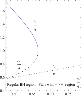
Figure 1: A plot of the several radii as a function of $\alpha=r_{0}/q$. The minimum value of $\alpha$ is $\sqrt{3}/3$, and the vertical dashed-dotted line is at $\alpha=2/3$.

Also,

$$Q(r)=q\,\theta(r-r_{0})\,,$$ (37)

$$Q^{\,\prime}(r)=q\,\delta(r-r_{0})\,,$$ (38)

$$\rho_{\rm e}(r)=\dfrac{q\,\sqrt{B(r_{0})}}{4\pi r_{0}^{2}}\,\delta(r-r_{0})\,,$$ (39)

$$\rho_{\rm m}(r)=\frac{q^{2}}{8\pi\,r_{0}^{4}}\left(1-\theta^{2}(r-r_{0})\right)\theta(r_{0}-r)\,,$$ (40)

$$p(r)=-\frac{q^{2}}{8\pi\,r_{0}^{4}}\left(1-\theta^{2}(r-r_{0})\right)\theta(r_{0}-r)\,,$$ (41)

$$p^{\,\prime}(r)=\frac{q^{2}}{4\,\pi\,r_{0}^{4}}\,\delta(r-r_{0})\,,$$ (42)

see Appendix B for how to obtain Eq. (42) from Eq. (41). Using the fact that $\theta^{2}(r-r_{0})=\theta(r-r_{0})$ (this can only be used if derivatives are not to be taken), Eqs. (40)-(41) simplify to $8\pi\,\rho_{\rm m}(r)=-8\pi\,p(r)=\displaystyle{\frac{3}{R^{2}}}\left[1-\theta(r-r_{0})\right].$

For a range of parameters, the solution represents regular black holes with a de Sitter core, and an electric energyless matter coat at $r_{0}$, and Reissner-Nordström all the way up. When there is no charge there is no regular black hole since for $q=0$ one has $r_{0}=0$ and $m=0$, leaving a Minkowski vacuum spacetime.

III.2.3 The solutions and their properties

Since we are not interested in the case $q=0$, as it gives the trivial Minkowski solution, we can parametrize all quantities in terms of $q$. Eq. (32) tell us that $r_{0}$ obeys, $r_{0}\geq\frac{q}{\sqrt{3}}$. Thus let us put

$$r_{0}={\alpha}\,q\,,$$ (43)

for some ${\alpha}$, with ${\alpha}\geq 1/\sqrt{3}$. Then, Eq. (30) gives

$$R={\sqrt{3}}{\alpha}^{2}\,q\,,$$ (44)

and Eq. (31) furnishes

$$m=\frac{2}{3{\alpha}}\,q\,.$$ (45)

Now, we have to compare $r_{0}$ with $r_{-}$ and $r_{+}$. These latter radii are given by

$$r_{\pm}=m\pm\sqrt{m^{2}-q^{2}}\,.$$ (46)

Putting Eq. (45) into Eq. (46) yields $r_{-}$ as

$$r_{-}=\left(\frac{2}{3{\alpha}}-\sqrt{\frac{4}{9{\alpha}^{2}}-1}\right)\,q\,,$$ (47)

and $r_{+}$ as

$$r_{+}=\left(\frac{2}{3{\alpha}}+\sqrt{\frac{4}{9{\alpha}^{2}}-1}\right)\,q\,.$$ (48)

A plot of the several radii as a function of $\alpha=r_{0}/q$ is given in Fig. 1.

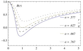
Figure 2: A plot of $B(r)$ for four different $\alpha\equiv\frac{r_{0}}{q}$: $\alpha=\sqrt{3}/3$ (solid line), $\alpha=\sqrt{3}/3+.1$ (dashed line), $\alpha=2/3$ (dash-dotted line), and $\alpha=2/3+.1$ (dotted line).

The solutions can be divided into four classes, which are listed and briefly discussed in the following. Figure 2 plots the function $B(r)$ and Figure 3 draws the Carter-Penrose diagrams for each class. Figures 1-3 help in the explanation of the classes.

(a) Regular nonextremal black holes

with a lightlike matter boundary at the inner horizon

When ${\alpha}=r_{0}/q$ has its minimum value $r_{0}/q=\sqrt{3}/3$, then the radius $r_{0}$ of the matter coincides with the Cauchy horizon $r_{-}$, so that $r_{-}/q=\sqrt{3}/3$. There is matter up to $r_{-}$. The event horizon at $r_{+}$ is at a larger radius. From Eq. (48) with ${\alpha}=\sqrt{3}/3$, one finds $r_{+}/q=3r_{-}/q=\sqrt{3}$. This is a solution for a perfectly regular black hole, Reissner-Nordström outside the matter. One can also find a relation between the surface charge density and the horizon radii. From Eq. (39) defining a proper surface electric charge density as $\rho_{\rm e}(r)=\sigma_{\rm e}\,\sqrt{B(r)}\,\delta(r-r_{0})$, one finds $\sigma_{\rm e}=\frac{q}{4\pi r_{0}^{2}}=\frac{1}{4\pi}\frac{3}{q}$. This can also be put in the form $\sigma_{\rm e}=\frac{1}{4\pi}\frac{\sqrt{3}}{r_{-}}$. Using $r_{+}/q=3r_{-}/q=\sqrt{3}$ and squaring the result, one obtains $\sigma_{\rm e}^{2}=\frac{1}{16\pi^{2}}\frac{r_{+}}{r_{-}^{3}}$. For this solution, in which $R^{2}=q^{2}/3$, one can show that the surface gravities of the de Sitter horizon and of the Cauchy Reissner-Nordström horizon are equal. The surface pressure and surface energy density are both zero at $r_{-}$.

(b) Regular nonextremal black holes

with a timelike matter boundary

inside the inner horizon

For larger $r_{0}/q$, i.e., larger $r_{0}$, the Cauchy horizon $r_{-}$ grows faster and remains outside the radius of the matter, $r_{0}<r_{-}$. There is matter up to $r_{0}$ and then outside the matter stand two horizons. This is also a solution for a perfectly regular black hole, Reissner-Nordström outside the matter.

Figure 3: The Carter-Penrose diagram in the possible four distinct situations, three for regular black holes and one for a star: (i) The regular nonextremal black hole with a lightlike matter boundary, where $r_{0}=r_{-}$. (ii) The regular nonextremal black hole with a timelike matter boundary, where $r_{0}<r_{-}$. (iii) The regular extremal black hole with a timelike matter boundary, where $r_{0}<r_{-}=r_{+}$. (iv) The regular overcharged star with a timelike matter boundary, where there is no $r_{\pm}$. In all cases, $r_{0}$ represents the surface matching an interior de Sitter spacetime region to an exterior Reissner-Nordström region. Note the regular black hole constraint $r_{0}\leq r_{-}$.

(c) Regular extremal black holes

with a timelike matter boundary

inside the double horizon

When $r_{0}/q=2/3$ then the Cauchy horizon and the event horizon coincide, the solution represents an extremal regular black hole. Since $r_{-}=r_{+}=m=q$ we have $r_{0}=\frac{2}{3}r_{+}$. The horizon is now at the furthest coordinate distance from the surface of the matter at $r_{0}$. In fact the horizon is at an infinite proper distance from the surface of the matter.

(d) Regular overcharged stars

with a timelike matter boundary

For $r_{0}/q>2/3$ one gets from Eq. (31) that $q>m$, the solution has charge greater than mass. Thus from Eq. (46) there are no horizons and so no black holes. An overcharged star, with no horizons, pops up. The star that was hidden behind a horizon comes into light. The horizons have disappeared. It is of remark that $r_{0}$ of the first star is still smaller than $r_{-}$ of the extremal regular black hole. Perhaps this is no surprise as we are familiar with the fact that the Reissner-Nordström solution has the same feature, after the extremal horizon the singularity at $r=0$ becomes bare for the overcharged solutions.

Several other features should be mentioned and emphasized.

(i) For a range of parameters the solutions are thus regular electrically charged black hole solutions. They are built from false vacuum up to, but not at, $r_{0}$. The metric for $r<r_{0}$ is the de Sitter metric, where the isotropic pressure is constant ($p(r)=-\rho_{\rm m}(r)=3/8\pi R^{2}$), and goes to zero at $r_{0}$. Furthermore, since the charge density $\rho_{\rm e}(r)$ is a Dirac delta function centered in $r=r_{0}$, the total charge $q$ is distributed uniformly on the surface $r=r_{0}$. At $r_{0}$ there is thus a thin electrical layer of an energyless field, and exterior to it it is pure Reissner-Nordström, with two horizons at $r_{-}$ and $r_{+}$. The radius to charge ratio and mass to charge ratio of the solution are well defined quantities.

(ii) From Eq. (45) we see that as $r_{0}$ increases the mass $m$ decreases. This is due to the fact that the pressure, and thus the density, both decrease fast as $r_{0}$ increases.

(iii) The limit of zero charge of these solutions is a Minkowski spacetime, rather than a Schwarzschild spacetime.

(iv) These regular charged black hole solutions have boundaries which are either timelike or, in one instance, lightlike. The boundaries for regular black holes found in the literature are spacelike.

(v) Note that, if the charge $q$ is the elementary charge, i.e., the electron charge $e$, then Eq. (32) gives that the radius $r_{0}$ of the particle is of the order of the Planck radius and from Eq. (33) the mass $m$ is of the order of the Planck mass. The solution could then be a model for a heavy elementary charged particle.

(vi) Due to the fact that the matter of the regular black hole is in the inside or at the Cauchy horizon, these solutions may suffer the mass inflation instability poisson1990 .

III.2.4 Comments on the regular nonextremal black hole with a lightlike matter boundary at the inner horizon $r_{-}$

Since the regular nonextremal black hole with a lightlike matter boundary at the inner horizon $r_{-}$ (see part (a) of Section III.2.3) has some history we comment on it. In (a) below we review and connect our solution to other works that also found this particular solution. In (b) we comment that this particular solution belongs to the Weyl-Guilfoyle class of solutions.

(a) Other works that also found this particular solution

As noticed in gron85 ; gronsol89 ; pisr88 ; gallem001 ; bron2001 a direct soldering of a matter solution onto Schwarzschild through the event horizon is not possible. Indeed, a simple calculation pisr88 shows that the radial pressure $p_{r}$ for a static spherically symmetric junction at $r=r_{0}$ is $p_{r}=-\rho_{\rm m}\theta(r_{0}-r)+\frac{1}{2}\rho_{\rm m}r_{0}\delta(r-r_{0})$. In terms of proper radial distance $s$, with $ds=\sqrt{A}\,dr$ (where $A$ is the metric function defined in (8)), the delta-function is $\delta(r-r_{0})={\sqrt{A}}\,\delta(s)$. At the Schwarzschild event horizon $1/A(r_{+})=0$, and thus the delta-function itself is a singular distribution. Thus, besides being a distribution, the surface pressure becomes singular when an event horizon is chosen as the boundary. Therefore, the papers gd81 ; sz88 ; stan89 ; daghig00 must be incorrect. A Schwarzschild event horizon is then not the place to make a continuation to a de Sitter phase, whereas other places might give a suitable continuation. However, when one introduces charge, and the matter is joined instead to a Reissner-Nordström spacetime, the impossibility of matching at the horizon can be avoided by making $\rho_{\rm m}=0$ and $p_{r}=0$ at the event horizon, as well as at the Cauchy horizon.

(i) The two papers by Shen and Zhu of 1985 on regular black holes with Reissner-Nordström asymptotics sz51 ; sz52 indeed contain, in a hidden manner, the regular nonextremal black hole with a lightlike matter boundary at the inner horizon $r_{-}$. Both papers sz51 ; sz52 have the same content, but oddly the authors do not self-cite neither paper. The paper sz52 is more detailed.

Shen and Zhu papers sz51 ; sz52 give a generalization of the Gonzalez-Diaz gd81 work (see also sz88 ; stan89 ), by considering the case with charge. In this way they avoid the matching problem. In sz51 ; sz52 it is claimed that by taking the limit of zero charge they recover the Gonzalez-Diaz gd81 solution. This claim seems incorrect since Eq. (34) of sz52 shows that in this limit there is a singularity at $r=0$, and so there is no regular Schwarzschild black hole.

Now, in a particular instance, the solution found in sz51 ; sz52 reduces to the regular nonextremal black hole with a lightlike matter boundary at the inner horizon $r_{-}$ found here. Let us see how. They consider two electrical coats, one at $r_{+}$, the other at $r_{-}$, such that $\rho_{1\rm e}=\sigma_{1\rm e}\delta(r-r_{+})$ and $\rho_{2\rm e}=\sigma_{2\rm e}\delta(r-r_{-})$, their Eqs. (17) and (18) respectively. They also find that the mass-density in between $r_{-}$ and $r_{+}$ is given in their Eq. (28), namely $\rho_{1\rm o}=\frac{3}{8\pi}\left[\frac{r_{+}-16\pi^{2}\sigma_{2\rm e}^{2}r_{-}^{3}}{r_{+}\left(r_{+}^{2}+r_{+}r_{-}+r_{-}^{2}\right)}\right]$, and the mass density between $0$ and $r_{-}$ is de Sitter type. There is an interesting special solution implicit in this solution. To find it one abolishes the matter existent in between $r_{-}$ and $r_{+}$. Impose $\rho_{1\rm e}=0$ and $\rho_{1\rm o}=0$. From $\rho_{1\rm e}=0$ nothing special comes about, but from $\rho_{1\rm o}=0$, one finds that $\sigma_{2\rm e}=\frac{1}{16\pi^{2}}\frac{r_{+}}{r_{-}^{3}}$. Then this solution is precisely our regular nonextremal black hole with a lightlike matter boundary at the inner horizon $r_{-}$, as one can check (see our part (a) of Section III.2.3).

(ii) The paper by Barrabès and Israel of 1991 barisrl91 also finds the regular nonextremal black hole with a lightlike matter boundary at the inner horizon $r_{-}$.

The direct matching conditions between an interior de Sitter region and an exterior Reissner-Nordström region having a lightlike surface as soldering surface was indeed considered by Barrabès and Israel barisrl91 (see also barrabes_hogan ). The authors have noticed that different matching conditions at a horizon are possible, and have given two special conditions, the static soldering and the affine soldering. In general, the soldering can be performed in anyone of the two horizons, but the surface pressure and energy density are nonzero. However, the static soldering offers a special case. When the de Sitter radius $R$ is related to the charge of the Reissner-Nordström solution $q$ by $R^{2}=q^{2}/3$, then the surface pressure and density are both zero and the surface gravities of the de Sitter horizon and of the Cauchy Reissner-Nordström horizon are equal. Here, of course, the matching happens at the inner horizon. This result agrees with what we have found above, but in our case, the matching can be done at any surface $r=r_{0}$, timelike if $r_{0}<r_{-}$, or lightlike if $r_{0}=r_{-}$. The solution is the same as the hidden solution in Shen and Zhu sz51 ; sz52 , and so the same as our particular solution.

(b) The solution is in the Weyl-Guilfoyle class of solutions

Charged star-type solutions found by Guilfoyle guilfoyle have a plethora of parameters from which one can choose values. These solutions contain quasiblack hole solutions as found by Lemos and Zanchin lemoszanchin2010 and it seems they also contain many different regular black holes. Here, we indicate that in a particular limit of those charged star-type solutions guilfoyle one obtains the regular nonextremal black holes with a lightlike matter boundary at the inner horizon mentioned in Sec. III.2.3(a).

Indeed, taking the parameter $A\to 0$ in Eq.  (25) of guilfoyle , or the limit $a\to\infty$ in lemoszanchin2010 as we do here, we find $\displaystyle{\lim_{a\to\infty}\dfrac{q^{2}}{m^{2}}=\frac{1}{2}\left(2+\left|\frac{r_{0}}{m}-2\right|-\frac{r_{0}}{m}\right)\frac{r_{0}}{m}}$. Due to the absolute value $\left|\frac{r_{0}}{m}-2\right|$ one concludes, remarkably, there are two branches, $\dfrac{r_{0}}{m}>2$ and $\dfrac{r_{0}}{m}<2$. For ${r_{0}}/{m}>2$ one finds ${\lim_{a\to\infty}\dfrac{q^{2}}{m^{2}}=0}$, which gives the uncharged Schwarzschild interior solution, and it is not of our concern here. For ${r_{0}}/{m}<2$ one finds ${\lim_{a\to\infty}\dfrac{q^{2}}{m^{2}}=\left(2-\frac{r_{0}}{m}\right)\frac{r_{0}}{m}}$, which is equivalent to $1-\frac{2m}{r_{0}}+\frac{q^{2}}{r_{0}^{2}}=0$. This branch is the one that interests us here, and we take the opportunity to make an analysis initiated in our previous paper lemoszanchin2010 in relation to this branch. The comments here take over the comments there. Thus $r_{0}$ is at a horizon, and consequently either at $r_{+}$ or $r_{-}$. Under closer scrutiny one finds that there is a special regular black hole solution among a maze of regular black hole solutions, in which $r_{0}=r_{-}$, $m=2r_{0}$, and $q=\sqrt{3}r_{0}$. This solution thus belongs to Guilfoyle’s class of solutions, i.e., it is a solution of Weyl-Guilfoyle type. Thus, this particular solution belongs to both Guilfoyle’s class of solutions and to a particular set of solutions we have been studying here. The other regular black holes and stars we have found here are not of Weyl-Guilfoyle type.

IV Conclusions

Charged regular black holes and overcharged stars as solutions to certain distributions of spherically symmetric charged matter have been displayed and studied. The interior distribution of matter is constituted by a de Sitter perfect fluid with pressure $p$ equal to the negative of the energy density $\rho_{\rm m}$. Thus, the interior can be interpreted as a false vacuum state. The interior metric is matched into an exterior Reissner-Nordström electrovacuum region. The Einstein-Maxwell equations together with the equation of state $p=-\rho_{\rm m}$, imply that the isotropic pressure and the energy density are constant throughout the spacetime, and that the electric charge must be located at the boundary of the fluid distribution. Pressure and energy density both go to zero at the boundary, and the resulting solutions represent regular charged black holes. The matter boundary is timelike, and in a limiting case is lightlike. The boundary surface is always at a radius smaller or, at most (in the lightlike case), equal to the inner Reissner-Nordström horizon. For overcharged matter a star pops up, and the horizons evanesce.

If the charge $q$ is the elementary charge $e$ then the mass of the solution is of the order of the Planck mass and the radius is of the order of the Planck radius. The solutions could then provide a model for a charged elementary Planckian particle.

Due to the fact that the matter of the regular black hole is in the inside or at the Cauchy horizon, these solutions may suffer the mass inflation instability.

In some models, such as in Dymnikova’s, the experimental investigation of physical processes occurring near the external event horizon could give some information about processes occurring deeply inside the black hole. Unfortunately, in our solution near the external event horizon there is no way to probe the inside of the black hole.

Appendix A The matching conditions on the boundary

We will follow israel to show that the boundary at $r_{0}$ is really a boundary surface. We need to show that the metric, or first fundamental form, $g_{\mu\nu}$ is continuous at the surface, $g_{\mu\nu}^{-}=g_{\mu\nu}^{+}$, or what is the same thing, $ds^{2}_{-}=ds^{2}_{+}$. It is also necessary that the extrinsic curvature, or second fundamental form, $K_{\mu\nu}$ is continuous, $K_{\mu\nu}^{-}=K_{\mu\nu}^{+}$.

For the surface $\Sigma$, defined by $r=r_{0}$, we adopt the metric

$$ds_{\Sigma}^{2}=-d\tau^{2}+r_{0}^{2}(d\theta^{2}+\sin^{2}d\phi^{2})\,,$$ (49)

with the intrinsic coordinates of $\Sigma$ being $\xi^{a}=(\tau,\theta,\phi)$, while the inner and the outer metrics are given receptively by (see Eqs. (34)-(35)),

$$ds_{-}^{2} = -\left(1-\frac{r^{2}}{R^{2}}\right)\,dt^{2}+\left(1-\frac{r^{2}}{R^{2}}\right)^{-1}dr^{2}$$ (50)

$$+\,r^{2}(d\theta^{2}+\sin^{2}d\phi^{2})\,,$$

and

$$ds_{+}^{2} = -\left(1-\frac{2m}{r}+\frac{q^{2}}{r^{2}}\right)\,dt^{2}+\left({1-\frac{2m}{r}+\frac{q^{2}}{r}}\right)^{-1}{dr^{2}}$$ (51)

$$+\,r^{2}(d\theta^{2}+\sin^{2}d\phi^{2})\,,$$

where we have identified the coordinates $(t,\,r,\,\theta,\,\varphi)$ in both regions of the spacetime.

Let us assume that the boundary surface $\Sigma$ is timelike, which means $1-r_{0}^{2}/R^{2}>0$ and also $1-2m/r_{0}+q^{2}/r_{0}^{2}>0$. Hence we note first that, since the surface $\Sigma$ is spherical and non-lightlike, the radial coordinate $r$ can be used as the matching parameter along the generators on $\Sigma$, and so the normal $n_{\mu}$ to the surface has only the radial component $n_{r}=\sqrt{g_{rr}}$. Therefore, in the present case the extrinsic curvature has the form

$$K_{ab}^{\pm}=-n^{\pm}_{r}\Gamma^{r(\pm)}_{\;\;\mu\nu}\;\frac{\partial x^{\mu}}{\partial\xi^{a}}\,\frac{\partial x^{\nu}}{\partial\xi^{b}}\,,$$ (52)

where $\xi^{a}$ are the intrinsic coordinates of the surface. Now we analyze the junction at the outer and inner surfaces. The continuity of the first fundamental form at the boundary implies that $g_{tt}^{+}=g_{tt}^{-}$ and $g_{rr}^{+}=g_{rr}^{-}$. These two conditions are satisfied by the continuity of the line elements given in Eqs. (50)-(51) at $r=r_{0}$, namely,

$$1-r_{0}^{2}/R^{2}=1-2m/r_{0}+q^{2}/r_{0}^{2}\,,$$ (53)

which is Eq. (20) and defines $R^{-2}$ in terms of the parameters $r_{0}$, $m$, and $q$. One then sees that the $g_{tt}^{+}$ and $g_{tt}^{-}$ match ant $r=r_{0}$, and $g_{rr}^{+}$ and $g_{rr}^{-}$ also match, as well as the terms for the angular part of the metric. Now, at $r_{0}$ coming from the interior one finds $K_{\tau\tau}^{-}=-n^{-}_{r}\,\Gamma^{(-)r}_{\;\;tt}\,\frac{dt}{d\tau}\frac{dt}{d\tau}$. By construction one has $g^{\pm}_{tt}\,\dfrac{dt^{2}}{d\tau^{2}}=-1$. One also has $n_{r}^{-}={1}/\sqrt{1-\frac{r_{0}^{2}}{R^{2}}}$. Noting that $\dfrac{dg_{tt}^{-}}{dr}=-\dfrac{2r_{0}}{R^{2}}$ one finds $\Gamma^{r(-)}_{\;\;tt}=\left(1-\dfrac{r_{0}^{2}}{R^{2}}\right)\dfrac{r_{0}}{R^{2}}$. Thus, $K_{\tau\tau}^{-}=-\sqrt{1-\dfrac{r_{0}^{2}}{R^{2}}\,}\dfrac{r_{0}}{R^{2}}$. Similarly, the extrinsic curvature coming from the exterior Reissner-Nordström region can also be calculated. One finds $K_{\tau\tau}^{+}=\sqrt{1-\dfrac{2m}{r_{0}}+\dfrac{q^{2}}{r_{0}^{2}}}\left(\dfrac{m}{r_{0}^{2}}-\dfrac{q^{2}}{r_{0}^{3}}\right)$. So, in order to match $K_{\tau\tau}^{+}$ and $K_{\tau\tau}^{-}$ the parameters $R$, $r_{0}$, $m$ and $q$ must satisfy the relation

$$\frac{r_{0}}{R^{2}}=-\frac{m}{r_{0}^{2}}+\frac{q^{2}}{r_{0}^{3}}\,.$$ (54)

This result, together with Eq. (53), gives

$$\frac{1}{R^{2}}=\frac{1}{3}\frac{q^{2}}{r_{0}^{4}}\,,$$ (55)

exactly the result found above (cf. Eq. (28)). This also means that the surface pressure vanishes. One can easily check that $K_{\theta\theta}$ and $K_{\phi\phi}$ also match. So the metric and the extrinsic curvature are continuous as is required. The electric potential $\phi$ is also continuous at the boundary as it is also required.

Let us assume that the boundary surface $\Sigma$ is lightlike now, which means $1-r_{0}^{2}/R^{2}>0$ and also $1-2m/r_{0}+q^{2}/r_{0}^{2}>0$. Then, the normal vector $n^{\mu}$ is lightlike. The radial coordinate $r$ cannot be used for the matching in this case. As it is proposed in barrabes_hogan (see also barisrl91 for the original work), an alternative is using the advanced (retarded) time $u$ as the soldering parameter, so that we can perform what Barrabès and Israel barisrl91 call a static soldering. The new coordinate $u$ is defined by

$$du = dt+\epsilon\frac{dr}{\left({1-\dfrac{r^{2}}{R^{2}}}\right)}\,,\quad\mbox{for }r<r_{0},$$ (56)

$$du = dt+\epsilon\frac{dr}{\left({1-\dfrac{2m}{r}+\dfrac{q^{2}}{r^{2}}}\right)}\,,\quad,\mbox{for}\;r>r_{0},$$ (57)

where $\epsilon=\pm 1$, and the plus (minus) sign is associated to the outgoing (ingoing) radial light rays on the cone $u=$ constant. The parameters on $\Sigma$ may be chosen as $\xi^{a}=(\tau=u,\,\theta,\,\varphi)$ barrabes_hogan ; barisrl91 . The normal to $\Sigma$ is therefore $n^{\mu}=\dfrac{\partial x^{\mu}}{\partial u}$, and, moreover, since $n^{\mu}$ is lightlike, an additional transverse vector $N^{\mu}$ is needed. This can be chosen as $N^{\mu}=\epsilon\dfrac{\partial x^{\mu}}{\partial r}$. Instead of the extrinsic curvature $K_{ab}$, the relevant quantity for a lightlike soldering is the transverse curvature ${\cal K}_{ab}$ defined by

$${\cal K}_{ab}=-N_{\mu}\Gamma^{\mu}_{\nu\rho}\frac{\partial x^{\nu}}{\partial\xi^{a}}\,\,\frac{\partial x^{\rho}}{\partial\xi^{b}}.$$ (58)

Then, the matching of the first fundamental form at $r=r_{0}$ gives $g_{uu}^{+}=g_{uu}^{-}$, which results in Eq. (53), is accomplished as far as that equality holds even in the limit of $r_{0}$ being a solution of the equations $1-r_{0}^{2}/R^{2}=0$ and $1-2m/r_{0}+q^{2}/r_{0}^{2}=0$, which is true in the particular case we are considering here. Moreover, calculating the nonzero components of ${\cal K}^{\pm}_{ab}$ we get

$${\cal K}^{+}_{uu}=\epsilon\left(\frac{m}{r_{0}^{2}}-\frac{q^{2}}{r_{0}^{3}}\right)\,,$$ (59)

$${\cal K}^{+}_{\theta\theta}={\cal K}^{+}_{\varphi\varphi}\sin^{-2}\theta={\epsilon}{r_{0}},$$ (60)

and

$${\cal K}^{-}_{uu}=-\epsilon\frac{r_{0}}{R^{2}}\,,$$ (61)

$${\cal K}^{-}_{\theta\theta}={\cal K}^{-}_{\varphi\varphi}\sin^{-2}\theta={\epsilon}{r_{0}},$$ (62)

where $r_{0}$ coincides with one of the horizons of the Reissner-Nordström spacetime. The matching between the metric coefficients on the horizon $r_{0}$ is clear. Again, imposing the continuity of the $uu$ component of transverse curvature, i.e., equating the relations (59) and (61) we find that they match only in the case $R=r_{0}=r_{-}$, $r_{-}$ being the inner Reissner-Nordström horizon. As a consequence of this matching, the pressure vanishes at the boundary surface, $p(r_{0})=0$. Note that here the lightlike case can be also analyzed as a limit of the configurations with a timelike boundary.

Appendix B How to obtain $p^{\prime}$

Note that the equation $\theta^{2}(r-r_{0})=\theta(r-r_{0})$ can only be used after taking derivatives. Also the Dirac delta function is given by $\delta(r-r_{0})=[\theta(r-r_{0})]^{\,\prime}$. Thus in Eq. (41) the term in front of $\dfrac{q^{2}}{r_{0}^{4}}$ differentiates to $\left[\theta^{2}(r-r_{0})\theta(r_{0}-r)\right]^{\,\prime}=2\theta(r-r_{0})\delta(r-r_{0})\theta(r_{0}-r)-\theta^{2}(r-r_{0})\delta(r-r_{0})=2\delta(r-r_{0})-\theta(r-r_{0})\delta(r-r_{0})=\delta(r-r_{0})$, where we have used $\theta(r-r_{0})\theta(r_{0}-r)=1$ in $r=r_{0}$ and zero otherwise, and $\theta(r-r_{0})\delta(r-r_{0})=\delta(r-r_{0})$. Now, the term in front of $-\dfrac{3}{R^{2}}$ has derivative $[\theta(r_{0}-r)]^{\,\prime}=-\delta(r-r_{0})$. Thus the whole term yields $+\dfrac{3}{R^{2}}\delta(r-r_{0})$. Since $\dfrac{3}{R^{2}}=\dfrac{q^{2}}{r_{0}^{4}}$ we have to sum both terms to give Eq. (42), i.e., $p^{\,\prime}(r)=\frac{q^{2}}{4\,\pi\,r_{0}^{4}}\,\delta(r-r_{0})$.

References

- (1) H. Stephani, D. Kramer, M. MacCallum, and C. Hoenselaers, Exact Solutions of Einstein’s Field Equations (Cambridge University Press, second edition, Cambridge 2002).
- (2) W. Israel, “Singular hypersurfaces and thin shells in general relativity”, Nuovo Cimento B 44, 1 (1966), erratum in Nuovo Cimento B 48, 463 (1967).
- (3) C. Barrabès and P. A. Hogan, Singular null hypersurfaces in General Relativity (World Scientific, Singapore, 2003).
- (4) C. W. Misner, K. S. Thorne, and J. A. Wheeler, Gravitation (Freeman, San Francisco, 1973).
- (5) J. B. Griffiths and J. Podolsky, Exact Space-Times in Einstein’s General Relativity (Cambridge University Press, Cambridge, 2009).
- (6) J. Stewart and M. Walker, “Black holes: the outside story”, in Astrophysics (Springer Tracts in Modern Physics Vol. 69), ed. G. Hohler (Springer-Verlag, Berlin, 1973), p. 69.
- (7) V. P. Frolov and I. D. Novikov, Black Hole Physics: Basic Concepts and New Developments (Kluwer Academic, Amsterdam, 1998).
- (8) R. Penrose, “Gravitational collapse and space-time singularities”, Phys. Rev. Lett. 14, 57 (1965).
- (9) S. Hawking and R. Penrose, “The singularities of gravitational collapse and cosmology”, Proc. Roy. Soc. London A 314, 529 (1970).
- (10) S. W. Hawking and G. F. R. Ellis, The Large Scale Structure of Space and Time (Cambridge University Press, Cambridge, 1973).
- (11) R. Penrose, “Singularities of spacetime”, in Theoretical Principles in Astrophysics and Relativity, eds. N. R. Lebovitz, W. H. Reid, and P. O. Vandervoort (Chicago University Press, Chicago, 1978), p. 217.
- (12) J. A. Wheeler, “Geometrodynamics and the issue of the final state”, in Relativity, groups, and topology, eds. C. DeWitt and B. DeWitt (Gordon and Breach, New York, 1964), p. 315.
- (13) A. D. Sakharov, “Initial stage of an expanding universe and appearance of a nonuniform distribution of matter”, Sov. Phys. JETP 22, 241 (1966).
- (14) E. Gliner, “Algebraic properties of the energy-momentum tensor and vacuum-like states of matter”, Sov. Phys. JETP 22, 378 (1966).
- (15) Y. B. Zel’dovich, “The cosmological constant and the theory of elementary particles”, Sov. Phys. Usp. 11, 381 (1968).
- (16) J. M. Bardeen, “Non-singular general-relativistic gravitational collapse”, in Proceedings of GR5 (Tbilisi, URSS, 1968).
- (17) E. B. Gliner and I. G. Dymnikova, “A nonsingular Friedman cosmology”, Sov. Astron. Lett. 1, 93 (1975).
- (18) I. G. Dymnikova, “Vacuum nonsingular black hole”, Gen. Relativ. Gravit. 24, 235 (1992).
- (19) I. G. Dymnikova, “De Sitter-Schwarzschild black hole: its particlelike core and thermodynamical properties”, Int. J. Mod. Phys. D 5, 529 (1996).
- (20) I. G. Dymnikova, “The algebraic structure of a cosmological term in spherically symmetric solutions”, Phys. Lett. B 472, 33 (2000); arXiv:gr-qc/9912116.
- (21) I. G. Dymnikova, A. Dobosz, M. L. Filchenkov, and A. Gromov, “Universes inside a Lambda black hole”, Phys. Lett. B 506, 351 (2001); arXiv:gr-qc/0102032.
- (22) I. G. Dymnikova, “Spherically symmetric space-time with regular de Sitter center”, Int. J. Mod. Phys. D 12, 1015 (2003); arXiv:gr-qc/0304110.
- (23) I. G. Dymnikova, “Regular electrically charged vacuum structures with de Sitter centre in nonlinear electrodynamics coupled to general relativity”, Classical Quantum Gravity 21, 4417 (2004); arXiv:gr-qc/0407072.
- (24) I. G. Dymnikova and E. Galaktionov, “Stability of a vacuum non-singular black hole”, Classical Quantum Gravity 22, 2331 (2005); arXiv:gr-qc/0409049.
- (25) I. G. Dymnikova and M. Korpusika, “Regular black hole remnants in de Sitter space”, Phys. Lett. B 685, 12 (2010).
- (26) E. B. Gliner, “Scalar Black Holes”, arXiv:gr-qc/9808042 (1998).
- (27) E. Ayón-Beato and A. García, “The Bardeen model as a nonlinear magnetic monopole”, Phys. Lett. B 493, 149 (2000); arXiv:gr-qc/0009077.
- (28) E. Ayón-Beato and A. García, “Four-parametric regular black hole solution”, Gen. Relativ. Gravit. 37, 635 (2005); arXiv:hep-th/0403229.
- (29) E. Ayón-Beato and A. García, “Regular black hole in general relativity coupled to nonlinear electrodynamics”, Phys. Rev. Lett. 80, 5056 (1998); arXiv:gr-qc/9911046.
- (30) K. A. Bronnikov, “Comment on ‘Regular Black Hole in General Relativity Coupled to Nonlinear Electrodynamics’ ”, Phys. Rev. Lett. 85, 4641 (2000).
- (31) K. A. Bronnikov, “Regular magnetic black holes and monopoles from nonlinear electrodynamics”, Phys. Rev. D 63, 044005 (2001); arXiv:gr-qc/0006014.
- (32) J. Matyjasek, “Extremal limit of the regular charged black holes in nonlinear electrodynamics”, Phys. Rev. D 70, 047504 (2004); arXiv:gr-qc/0403109.
- (33) K. A. Bronnikov and J. C. Fabris, “Regular Phantom Black Holes”, Phys. Rev. Lett. 96, 251101 (2006); arXiv:gr-qc/0511109 .
- (34) K. A. Bronnikov, H. Dehnen, and V. N. Melnikov, “Regular black holes and black universes”, Gen. Relativ. Gravit. 39, 973 (2007); arXiv:gr-qc/0611022.
- (35) K. A. Bronnikov and I. Dymnikova, “Regular homogeneous T-models with vacuum dark fluid”, Classical Quantum Gravity 24, 5803 (2007); arXiv:0705.2368 [gr-qc].
- (36) J. Matyjasek, D. Tryniecki, and M. Klimek, “Regular black holes in an asymptotically de Sitter universe”, Mod. Phys. Lett. A 23, 3377 (2009); arXiv:0809.2275 [gr-qc].
- (37) W. Berej, J. Matyjasek, D. Tryniecki, and M. Woronowicz, “Regular black holes in quadratic gravity”, Gen. Relativ. Gravit. 38, 885 (2006); arXiv:hep-th/0606185.
- (38) M. Mars, M. M. Martin-Prats, and J. M. M. Senovilla, “Models of regular Schwarzschild black holes satisfying weak energy conditions”, Classical Quantum Gravity 13, L51 (1996).
- (39) G. Magli, “Physically valid black hole interior models”, Rep. Math. Phys. 44, 407 (1999); arXiv:gr-qc/9706083.
- (40) S. Conboy and K. Lake, “Smooth transitions from Schwarzschild vacuum to de Sitter space”, Phys. Rev. D 71, 124017 (2005); arXiv:gr-qc/0504036.
- (41) E. Elizalde and S. R. Hildebrandt, “Family of regular interiors for nonrotating black holes with ”, Phys. Rev. D 65, 124024 (2002); arXiv:gr-qc/0202102.
- (42) M. A. Markov, “Problems of a Perpetually Oscillating Universe”, Ann. Phys. (New York) 155, 333 (1984).
- (43) V. P. Frolov, M. A. Markov, and V. F. Mukhanov, “Black holes as possible sources of closed and semiclosed worlds”, Phys. Rev. D 41, 383 (1990).
- (44) C. Barrabes and V. P. Frolov, “How many new worlds are inside a black hole?”, Phys. Rev. D 53, 3215 (1996); arXiv:hep-th/9511136.
- (45) D. Morgan, “Black holes in cutoff gravity”, Phys. Rev. D 43, 3144 (1991).
- (46) R. Balbinot and E. Poisson, “Stability of the Schwarzschild-de Sitter model”, Phys. Rev. D 41, 395 (1990).
- (47) R. Balbinot, “Scalar field in the Frolov-Markov-Mukhanov black hole spacetimes”, Phys. Rev. 41, 1810 (1990).
- (48) K. Lake and T. Zannias, “Fitting de Sitter space into a black hole”, Phys. Lett. A 140, 291 (1989).
- (49) A. Burinskii, E. Elizalde, S. R. Hildebrandt, and G. Magli, “Regular sources of the Kerr-Schild class for rotating and nonrotating black hole solutions”, Phys. Rev. D 65, 064039 (2002); arXiv:gr-qc/0109085.
- (50) P. F. Gonzales-Diaz, “The space-time metric inside a black hole”, Lett. Nuovo Cimento 32, 161 (1981).
- (51) W. Shen and S. Zhu, “Junction conditions on null hypersurface”, Phys. Lett. A 126, 229 (1988).
- (52) Y. G. Shen and Z. Q. Tan, “Global regular solution in higher-dimensional Schwarzschild spacetime”, Phys. Lett. A 142, 341 (1989).
- (53) R. G. Daghigh, J. I. Kapusta, and Y. Hosotani, “False vacuum black holes and Universes”, arXiv:gr-qc/0008006 (2000).
- (54) Ø. Grøn, “Space-time inside a black hole”, Lett. Nuovo Cimento 44, 177 (1985).
- (55) Ø. Grøn and H. H. Soleng, “Dynamical instability of the Gonzalez-Diaz black hole model”, Phys. Lett. A 138, 89 (1989).
- (56) E. Poisson and W. Israel, “Structure of the black hole nucleus”, Classical Quantum Gravity 5, L201 (1988).
- (57) D. V. Gal’tsov and J. P. S. Lemos, “No-go theorem for false vacuum black holes”, Classical Quantum Gravity 18, 1715 (2001); arXiv:gr-qc/0008076.
- (58) K. A. Bronnikov, “Spherically symmetric false vacuum: No-go theorems and global structure”, Phys. Rev. D 64, 064013 (2001); arXiv:gr-qc/0104092.
- (59) W. Shen and S. Zhu, “Globally regular solutions of a Schwarzschild black hole and a Reissner-Nordström black hole”, Gen. Relativ. Gravit. 17, 739 (1985).
- (60) W. Shen and S. Zhu, “The space-time metric inside a charged black hole”, Nuovo Cimento B 85, 142 (1985).
- (61) C. Barrabès and W. Israel, “Thin Shells in General relativity and Cosmology: the Lightlike Limit”, Phys. Rev. D 43, 1129 (1991).
- (62) A. Borde, “Open and closed universes, initial singularities, and inflation”, Phys. Rev. D 50, 3692 (1994); arXiv:gr-qc/9403049.
- (63) A. Borde, “Regular black holes and topology change”, Phys. Rev. D 55, 7615 (1997); arXiv:gr-qc/9612057.
- (64) M. Mars, M. M. Martín-Prats, and J. M. M. Senovilla, “The property of spherically symmetric static spacetimes”, Phys. Lett. A 218, 147 (1996).
- (65) O. B. Zaslavskii, “Regular black holes with flux tube core”, Phys. Rev. D 80, 064034 (2009); arXiv:0909.2270 [gr-qc].
- (66) O. B. Zaslavskii, “Regular black holes and energy conditions”, Phys. Lett. B 688, 278 (2010); arXiv:1004.2362 [gr-qc].
- (67) L. Balart, “Quasilocal energy, Komar charge and horizon for regular black holes”, Phys. Lett. B 687, 280 (2010), arXiv:0912.0334 [gr-qc].
- (68) Y. S. Myung, Y. W. Kim, and Y. J. Park, “Entropy of an extremal regular black hole”, Phys. Lett. B 659, 832 (2008); arXiv:0705.2478 [gr-qc].
- (69) Y. S. Myung, Y. W. Kim, and Y. J. Park, “Thermodynamics of regular black hole”, Gen. Relativ. Gravit. 41, 1051 (2008); arXiv:0708.3145 [gr-qc].
- (70) S. Ansoldi, “Spherical black holes with regular center: a review of existing models including a recent realization with Gaussian sources”, arXiv:0802.0330 [gr-qc] (2008).
- (71) J. P. S. Lemos and O. B. Zaslavskii, “Quasiblack holes: definition and general properties”, Phys. Rev. D 76, 084030 (2007); arXiv:0707.1094 [gr-qc].
- (72) B. S. Guilfoyle, “Interior Weyl-type solutions to the Einstein-Maxwell field equations”, Gen. Relativ. Gravit. 31, 1645 (1999); arXiv:gr-qc/9906089.
- (73) J. P. S. Lemos and V. T. Zanchin, “Quasiblack holes with pressure: relativistic charged spheres as the frozen stars”, Phys. Rev. D 81, 124016 (2010); arXiv:1004.3574 [gr-qc].
- (74) S. K. Blau, E. I. Guendelman, and A. H. Guth, ”Dynamics of false-vacuum bubbles”, Phys. Rev. D 35, 1747 (1987).
- (75) V. A. Berezin, V. A. Kuzmin, and I. I. Tkachev, “Dynamics of bubbles in general relativity”, Phys. Rev. D 36, 2919 (1987).
- (76) G. L. Alberghi, D. A. Lowe, and M. Trodden, “Charged False Vacuum Bubbles and the AdS/CFT Correspondence”, JHEP 9907, 020 (1999); arXiv:hep-th/9906047.
- (77) E. Poisson and W. Israel, “Internal structure of black holes”, Phys. Rev. D 41, 1796 (1990).