On the experimental violation of Mermin’s inequality with imperfect measurements

Ruffin Evans    Olivier Pfister opfister@virginia.edu Department of Physics, University of Virginia, 382 McCormick Rd., Charlottesville, VA 22903, USA
Abstract

We investigate theoretically the feasibility of an experimental test of the Bell-type inequality derived by Mermin for correlated spins larger than 1/212{1}/{2}. Using the Schwinger representation, we link the output fields of two two-mode squeezers in order to create correlated effective spins between two observers. Spin measurements will be performed by photon-number-resolved photodetection, which has recently come of age. We examine the effect of nonideal detection quantum efficiency—and any other optical loss—on the violation margin of Mermin’s inequality. We find that experimental violation is well accessible for spins larger than 1 for quantum efficiencies compatible with the current state of the art.

I Introduction

The violation of Bell inequalities Bell1964 by measurements on quantum correlated systems with spins larger than the original 1/212{1}/{2} value is of interest as a test of a new quantum regime, and possibly as a test of the quantum to classical transition Mermin1980 . In 1980, David Mermin showed that the “standard” Bell inequality cannot be violated for spins larger than 1/212{1}/{2} and derived an alternative inequality which is violated by quantum mechanics for higher spins Mermin1980 . More recently, Collins, Gisin, Linden, Massar, and Popescu (CGLMP) discovered a generic method to investigate locality violations for higher-dimensional systems Collins2002 —Qdits rather than Qbits Mermin2003 —that may also offer increased violation and resistance to loss.

Classic spin-1/212{1}/{2} Bell inequalities have been violated under a variety of conditions over the past five decades. In particular, important experiments have closed various loopholes, such as the locality loophole Aspect1982 ; Aspect1982a ; Weihs1998 , the fair sampling loophole Rowe2001 , and, most recently, the freedom-of-choice loophole Scheidl2010 .

In this paper, our motivation is to pave the way for an experimental test of Bell-type inequalities for spins larger than 1/212{1}/{2} in general. An experimental violation of Bell inequalities for spin-1 systems was demonstrated Howell2002 but no other experimental work has been conducted on this subject to our knowledge. Here, we study an experimental protocol that was proposed earlier by Reid and Drummond Drummond1983 ; Reid2002 , albeit in the context of dichotomic (Qbit) measurements. A related but different proposal was also made by Gerry and Albert Gerry2005 . This protocol (detailed in Section II) consists in using two pairs of entangled optical fields shared between two observers and viewed, in the Schwinger representation Schwinger1965 , as 2 spin s𝑠s particles in the zero-spin state used by Mermin’s high-dimensional Bell inequality. Here, we are interested in the experimental feasibility of violating Mermin’s inequality for s>1𝑠1s>1 and focus on a realistic model that includes arbitrary photodetection losses. This model is computationally intensive, hence we will focus solely on Mermin’s inequality, which is the simplest computationally, even though an investigation of the CGLMP inequality (among others) is an equally interesting goal for future work.

I.1 An example

Despite the relative simplicity of Bell’s original inequality, it resists straightforward generalization to higher spins, as was pointed out by Mermin Mermin1980 . A good illustration of the situation is provided by examining the Clauser-Horne-Shimony-Holt (CHSH) inequality Clauser1969 , which can be constructed by taking the results of the measurements, by Alice and Bob respectively, of the components of two spins Sasubscript𝑆𝑎\vec{S}_{a} and Sbsubscript𝑆𝑏\vec{S}_{b} along axes denoted by angles α𝛼\alpha, β𝛽\beta, γ𝛾\gamma, and δ𝛿\delta about the z𝑧z axis Peres1995 :

𝒞𝒞\displaystyle\mathcal{C} =|mA,α+mA,γ|mB,β+|mA,αmA,γ|mB,δabsentsubscript𝑚𝐴𝛼subscript𝑚𝐴𝛾subscript𝑚𝐵𝛽subscript𝑚𝐴𝛼subscript𝑚𝐴𝛾subscript𝑚𝐵𝛿\displaystyle=\left|m_{A,\alpha}+m_{A,\gamma}\right|m_{B,\beta}+\left|m_{A,\alpha}-m_{A,\gamma}\right|m_{B,\delta} (1)

For spins 1/212{1}/{2}, and normalizing the measurement results to values of ±1plus-or-minus1\pm 1, it is easy to show that

𝒞2.𝒞2\mathcal{C}\leqslant 2. (2)

However, as is well known, this counterfactual CHSH inequality is violated by quantum mechanics, which allows 𝒞𝑚𝑎𝑥=22subscript𝒞𝑚𝑎𝑥22\mathcal{C}_{\mathit{max}}=2\sqrt{2} for select angles when the spins are in a maximally entangled state. Let’s now consider the general case of 2 spins s𝑠s. It is relatively easy to show that, in this case, a counterfactual inequality is

𝒞𝒞\displaystyle\mathcal{C} 2s2absent2superscript𝑠2\displaystyle\leqslant 2s^{2} (3)

Like in the spin 1/212{1}/{2} case, we now consider the quantum state of total spin 0

|(ss) 00=12s+1m=ss(1)sm|s,ma|s,mb,ket𝑠𝑠0012𝑠1superscriptsubscript𝑚𝑠𝑠superscript1𝑠𝑚subscriptket𝑠𝑚𝑎subscriptket𝑠𝑚𝑏\left|\,(ss)\,00\,\right\rangle=\frac{1}{\sqrt{2s+1}}\sum_{m=-s}^{s}(-1)^{s-m}\left|\,s,m\,\right\rangle_{a}\left|\,s,-m\,\right\rangle_{b}, (4)

for which the spin correlation matrix elements take the simple form Mermin1980

SA,αSB,β=13s(s+1)cos(αβ).delimited-⟨⟩subscript𝑆𝐴𝛼subscript𝑆𝐵𝛽13𝑠𝑠1𝛼𝛽\left\langle S_{A,\alpha}S_{B,\beta}\right\rangle=-\frac{1}{3}s(s+1)\cos(\alpha-\beta). (5)

In this case the CHSH inequality becomes

|cos(αβ)+cos(γβ)+cos(αδ)cos(γδ)|6ss+1.𝛼𝛽𝛾𝛽𝛼𝛿𝛾𝛿6𝑠𝑠1\displaystyle\left|\cos(\alpha-\beta)+\cos(\gamma-\beta)\right.+\left.\cos(\alpha-\delta)-\cos(\gamma-\delta)\right|\leqslant\frac{6s}{s+1}. (6)

The absolute value on the left-hand side of Eq. (6) is bounded from above by 22222\sqrt{2}, which corresponds to the maximum violation that quantum mechanics can offer. In that case, the inequality becomes

s232=0.89,𝑠2320.89s\geqslant\frac{\sqrt{2}}{3-\sqrt{2}}=0.89, (7)

which is clearly satisfied by s>1/2𝑠12s>1/2. These spin values therefore pass the CHSH locality test.

However, this simple example should only be regarded as the tree that masks the forest. Indeed, there are many Bell-type inequalities that are violated by quantum mechanics for higher spins. Reference Howell2002 gives an instance for s=1𝑠1s=1, along with an experimental violation, and the aforementioned Refs. Mermin1980 ; Collins2002 do so for arbitrary s𝑠s. Moreover, work has also been done on Bell inequalities involving higher-dimensional systems in terms of dichotomic-variable measurements (e.g. photon-counting thresholds, photon-number parity) Drummond1983 ; Gisin1992 ; Banaszek1998 ; Reid2002 .

I.2 Mermin’s inequality Mermin1980

We now recall Mermin’s counterfactual inequality, which is violated by quantum mechanics in the zero eigenstate of the total spin:

s|mA,αmB,β|𝑎𝑣mA,αmB,γ𝑎𝑣+mA,βmB,γ𝑎𝑣𝑠subscriptdelimited-⟨⟩subscript𝑚𝐴𝛼subscript𝑚𝐵𝛽𝑎𝑣subscriptdelimited-⟨⟩subscript𝑚𝐴𝛼subscript𝑚𝐵𝛾𝑎𝑣subscriptdelimited-⟨⟩subscript𝑚𝐴𝛽subscript𝑚𝐵𝛾𝑎𝑣s\langle|m_{A,\alpha}-m_{B,\beta}|\rangle_{\mathit{av}}\geqslant\langle m_{A,\alpha}m_{B,\gamma}\rangle_{\mathit{av}}+\langle m_{A,\beta}m_{B,\gamma}\rangle_{\mathit{av}} (8)

where

s|mA,αmB,β|𝑎𝑣=m,m|mm|P(m,m,αβ).𝑠subscriptdelimited-⟨⟩subscript𝑚𝐴𝛼subscript𝑚𝐵𝛽𝑎𝑣subscript𝑚superscript𝑚𝑚superscript𝑚𝑃𝑚superscript𝑚𝛼𝛽s\langle|m_{A,\alpha}-m_{B,\beta}|\rangle_{\mathit{av}}=\sum_{m,m^{\prime}}|m-m^{\prime}|P(m,m^{\prime},\alpha-\beta). (9)

In the quantum mechanical derivation, the zero-spin state of Eq. (4) yields

P(m,m,αβ)=12s+1|m|ei(αβπ)Sy|m|2=|dmms(α+β+π)|22s+1𝑃𝑚superscript𝑚𝛼𝛽12𝑠1superscriptquantum-operator-product𝑚superscript𝑒𝑖𝛼𝛽𝜋subscript𝑆𝑦superscript𝑚2superscriptsubscriptsuperscript𝑑𝑠𝑚superscript𝑚𝛼𝛽𝜋22𝑠1P(m,m^{\prime},\alpha-\beta)=\frac{1}{2s+1}\left|\left\langle\,m\,\right|e^{i(\alpha-\beta-\pi)S_{y}}\left|\,m^{\prime}\,\right\rangle\right|^{2}=\frac{|d^{s}_{mm^{\prime}}(-\alpha+\beta+\pi)|^{2}}{2s+1} (10)

and, as aforementioned in Eq. (5),

mA,αmB,γ𝑎𝑣=SA,αSB,β=13s(s+1)cos(αβ),subscriptdelimited-⟨⟩subscript𝑚𝐴𝛼subscript𝑚𝐵𝛾𝑎𝑣delimited-⟨⟩subscript𝑆𝐴𝛼subscript𝑆𝐵𝛽13𝑠𝑠1𝛼𝛽\langle m_{A,\alpha}m_{B,\gamma}\rangle_{\mathit{av}}=\left\langle S_{A,\alpha}S_{B,\beta}\right\rangle=-\frac{1}{3}s(s+1)\cos(\alpha-\beta), (11)

In evaluating the violation of Eq. (8), Mermin computed (numerical) optimal measurement angles for maximal violation. The formulas above assume perfect measurements. In this work, we generalized Mermin’s inequality to include the effect of measurement inefficiency in a particular optical implementation. The paper is organized as follows. In Section 2, we detail our experimental implementation proposal. In Section 3, we introduce our loss decoherence (detection quantum efficiency η𝜂\eta) model and apply it to Mermin’s inequality. In Section 4, we present the results of our numerical evaluations for s=1/2𝑠12s=1/2 to 9/2929/2 and η=0.4𝜂0.4\eta=0.4 to 1. We then conclude.

II Proposed experimental implementation

II.1 Einstein-Podolsky-Rosen (EPR) entanglement between Alice and Bob

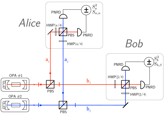
We consider the experimental setup sketched in Fig. 1. Two two-mode squeezers, or optical parametric amplifiers OPA#1 and OPA#2, are realized by using two optical parametric oscillators (OPOs) below threshold.
Refer to caption

Figure 1: Proposed experimental setup for the violation of Mermin’s inequality. OPA: optical parametric amplifier. PBS: polarizing beamsplitter. HWP: halfwave plate. PNRD: photon-number-resolving detector. Note that all optical paths in air between two consecutive PBS must be in phase, except for that of a2subscript𝑎2a_{2} which must be exactly out of phase.

Each OPA emits a two-mode squeezed, or EPR, state and each entangled mode is sent to each partner, Alice and Bob. Alice and Bob therefore each receive two independent fields, and each of their two fields is entangled with one of their partner’s fields. This double EPR state is Walls1994

|EPR2=ket𝐸𝑃superscript𝑅2absent\displaystyle\left|\,EPR^{2}\,\right\rangle= n1=0(tanhr1)n1coshr1|n1A1|n1B1n2=0(tanhr2)n2coshr2|n2A2|n2B2,superscriptsubscriptsubscript𝑛10tensor-productsuperscriptsubscript𝑟1subscript𝑛1subscript𝑟1subscriptketsubscript𝑛1𝐴1subscriptketsubscript𝑛1𝐵1superscriptsubscriptsubscript𝑛20superscriptsubscript𝑟2subscript𝑛2subscript𝑟2subscriptketsubscript𝑛2𝐴2subscriptketsubscript𝑛2𝐵2\displaystyle\sum_{n_{1}=0}^{\infty}\frac{(\tanh r_{1})^{n_{1}}}{\cosh r_{1}}\left|\,n_{1}\,\right\rangle_{A1}\left|\,n_{1}\,\right\rangle_{B1}\otimes\sum_{n_{2}=0}^{\infty}\frac{(\tanh r_{2})^{n_{2}}}{\cosh r_{2}}\left|\,n_{2}\,\right\rangle_{A2}\left|\,n_{2}\,\right\rangle_{B2}, (12)

where r1,2subscript𝑟12r_{1,2} are the squeezing parameters. We now show how this state can be recast as a perfectly entangled spin state, even for finite values of r1,2subscript𝑟12r_{1,2}. This was first pointed out by Drummond Drummond1983 and Reid et al. Reid2002 .

II.2 Spin entanglement between Alice and Bob

We use the Schwinger representation Schwinger1965 , which consists in defining the following effective spin operators

SAxsubscript𝑆𝐴𝑥\displaystyle S_{Ax} =12(a1a2+a1a2)absent12subscriptsuperscript𝑎1subscript𝑎2subscript𝑎1subscriptsuperscript𝑎2\displaystyle=\frac{1}{2}\left(a^{\dagger}_{1}a_{2}+a_{1}a^{\dagger}_{2}\right) (13)
SAysubscript𝑆𝐴𝑦\displaystyle S_{Ay} =12i(a1a2a1a2)absent12𝑖subscriptsuperscript𝑎1subscript𝑎2subscript𝑎1subscriptsuperscript𝑎2\displaystyle=\frac{1}{2i}\left(a^{\dagger}_{1}a_{2}-a_{1}a^{\dagger}_{2}\right) (14)
SAzsubscript𝑆𝐴𝑧\displaystyle S_{Az} =12(a1a1a2a2)absent12subscriptsuperscript𝑎1subscript𝑎1subscriptsuperscript𝑎2subscript𝑎2\displaystyle=\frac{1}{2}\left(a^{\dagger}_{1}a_{1}-a^{\dagger}_{2}a_{2}\right) (15)
SA2superscriptsubscript𝑆𝐴2\displaystyle S_{A}^{2} =a1a1+a2a22(a1a1+a2a22+1)absentsubscriptsuperscript𝑎1subscript𝑎1subscriptsuperscript𝑎2subscript𝑎22subscriptsuperscript𝑎1subscript𝑎1subscriptsuperscript𝑎2subscript𝑎221\displaystyle=\frac{a^{\dagger}_{1}a_{1}+a^{\dagger}_{2}a_{2}}{2}\left(\frac{a^{\dagger}_{1}a_{1}+a^{\dagger}_{2}a_{2}}{2}+1\right) (16)

for Alice, and

SBxsubscript𝑆𝐵𝑥\displaystyle S_{Bx} =12(b2b1+b2b1)absent12subscriptsuperscript𝑏2subscript𝑏1subscript𝑏2subscriptsuperscript𝑏1\displaystyle=\frac{1}{2}\left(b^{\dagger}_{2}b_{1}+b_{2}b^{\dagger}_{1}\right) (17)
SBysubscript𝑆𝐵𝑦\displaystyle S_{By} =12i(b2b1b2b1)absent12𝑖subscriptsuperscript𝑏2subscript𝑏1subscript𝑏2subscriptsuperscript𝑏1\displaystyle=\frac{1}{2i}\left(b^{\dagger}_{2}b_{1}-b_{2}b^{\dagger}_{1}\right) (18)
SBzsubscript𝑆𝐵𝑧\displaystyle S_{Bz} =12(b2b2b1b1)absent12subscriptsuperscript𝑏2subscript𝑏2subscriptsuperscript𝑏1subscript𝑏1\displaystyle=\frac{1}{2}\left(b^{\dagger}_{2}b_{2}-b^{\dagger}_{1}b_{1}\right) (19)
SB2superscriptsubscript𝑆𝐵2\displaystyle S_{B}^{2} =b1b1+b2b22(b1b1+b2b22+1)absentsubscriptsuperscript𝑏1subscript𝑏1subscriptsuperscript𝑏2subscript𝑏22subscriptsuperscript𝑏1subscript𝑏1subscriptsuperscript𝑏2subscript𝑏221\displaystyle=\frac{b^{\dagger}_{1}b_{1}+b^{\dagger}_{2}b_{2}}{2}\left(\frac{b^{\dagger}_{1}b_{1}+b^{\dagger}_{2}b_{2}}{2}+1\right) (20)

for Bob. It is easy to check that these operators satisfy the canonical commutation relations of a quantum angular momentum. The usual eigenstates are those of (S2,Sz)superscript𝑆2subscript𝑆𝑧(S^{2},S_{z}):

|sA,mAA=|nA1+nA22,nA1nA22Asubscriptketsubscript𝑠𝐴subscript𝑚𝐴𝐴subscriptketsubscript𝑛𝐴1subscript𝑛𝐴22subscript𝑛𝐴1subscript𝑛𝐴22𝐴\left|\,s_{A},m_{A}\,\right\rangle_{A}=\left|\,\frac{n_{A1}+n_{A2}}{2},\frac{n_{A1}-n_{A2}}{2}\,\right\rangle_{A}\\ (21)

for Alice, and

|sB,mBB=|nB1+nB22,nB1nB22Bsubscriptketsubscript𝑠𝐵subscript𝑚𝐵𝐵subscriptketsubscript𝑛𝐵1subscript𝑛𝐵22subscript𝑛𝐵1subscript𝑛𝐵22𝐵\left|\,s_{B},m_{B}\,\right\rangle_{B}=\left|\,\frac{n_{B1}+n_{B2}}{2},\frac{n_{B1}-n_{B2}}{2}\,\right\rangle_{B} (22)

for Bob. They can be measured in a straightforward manner if one can count photons with unity efficiency. The detectors in Fig. 1 will be photon-number-resolving superconducting transition-edge sensors, which have been installed in our laboratory at the University of Virginia, in collaboration with the groups of Sae Woo Nam at the National Institute of Standards and Technology and Aaron Miller at Albion College. Such detectors have been shown to allow photon-number resolution at quantum efficiencies exceeding 95% Lita2008 .

It is worthwhile to make explicit the physical meaning of these effective spin observables. Unsurprisingly, the total rotational energies given by observables SA,B2superscriptsubscript𝑆𝐴𝐵2S_{A,B}^{2} coincide with the total energy in Alice’s and Bob’s fields, respectively. The spin projection along z𝑧z coincides with the photon number difference between the two fields on one partner’s side. Finally, it is straightforward to see that the physical meaning of the spin projections along x𝑥x and y𝑦y is simply the phase difference between the two fields on one partner’s side, since the observables Sx,ysubscript𝑆𝑥𝑦S_{x,y} are clearly interference terms. These considerations therefore completely specify the measurement procedure Kim1998 , which we detail in the next subsection.

We can thus rewrite the double EPR state as

|EPR2=s=0m=ss(tanhr1)s+mcoshr1(tanhr2)smcoshr2|smA|smB.ket𝐸𝑃superscript𝑅2superscriptsubscript𝑠0superscriptsubscript𝑚𝑠𝑠superscriptsubscript𝑟1𝑠𝑚subscript𝑟1superscriptsubscript𝑟2𝑠𝑚subscript𝑟2subscriptket𝑠𝑚𝐴subscriptket𝑠𝑚𝐵\left|\,EPR^{2}\,\right\rangle=\sum_{s=0}^{\infty}\sum_{m=-s}^{s}\frac{(\tanh r_{1})^{s+m}}{\cosh r_{1}}\frac{(\tanh r_{2})^{s-m}}{\cosh r_{2}}\left|\,s\ m\,\right\rangle_{A}\left|\,s\ -m\,\right\rangle_{B}. (23)

This state can be put in an interesting form provided the squeezing parameters are identical r1=r2=rsubscript𝑟1subscript𝑟2𝑟r_{1}=r_{2}=r. We then obtain

|EPR2=s=0[(tanhr)scoshr]2m=ss|smA|smB.ket𝐸𝑃superscript𝑅2superscriptsubscript𝑠0superscriptdelimited-[]superscript𝑟𝑠𝑟2superscriptsubscript𝑚𝑠𝑠subscriptket𝑠𝑚𝐴subscriptket𝑠𝑚𝐵\left|\,EPR^{2}\,\right\rangle=\sum_{s=0}^{\infty}\left[\frac{(\tanh r)^{s}}{\cosh r}\right]^{2}\sum_{m=-s}^{s}\left|\,s\ m\,\right\rangle_{A}\left|\,s\ -m\,\right\rangle_{B}. (24)

This state is clearly a maximally entangled spin state at any given value of s𝑠s, which can be heralded or defined by the measurement of the total photon number on Alice’s and Bob’s sides. In addition, we can obtain the exact zero-total-spin eigenstate by phase shifting either the A2𝐴2A2 or the B2𝐵2B2 optical path by π𝜋\pi:

eiπNA2|n2A2=eiπn2|n2A2=(1)n2|n2A2,superscript𝑒𝑖𝜋subscript𝑁𝐴2subscriptketsubscript𝑛2subscript𝐴2superscript𝑒𝑖𝜋subscript𝑛2subscriptketsubscript𝑛2subscript𝐴2superscript1subscript𝑛2subscriptketsubscript𝑛2subscript𝐴2e^{-i\pi N_{A2}}\left|\,n_{2}\,\right\rangle_{A_{2}}=e^{-i\pi n_{2}}\left|\,n_{2}\,\right\rangle_{A_{2}}=(-1)^{n_{2}}\left|\,n_{2}\,\right\rangle_{A_{2}},

which yields

|EPR2=s=02s+1[(tanhr)scoshr]2|(ss)00.ket𝐸𝑃superscript𝑅2superscriptsubscript𝑠02𝑠1superscriptdelimited-[]superscript𝑟𝑠𝑟2ket𝑠𝑠00\left|\,EPR^{2}\,\right\rangle=\sum_{s=0}^{\infty}\sqrt{2s+1}\left[\frac{(\tanh r)^{s}}{\cosh r}\right]^{2}\left|\,(ss)00\,\right\rangle. (25)

Thus, the double EPR state can be made equivalent to the eigenstate of two spins s𝑠s coupled into a zero total spin. Do note that the maximal entanglement of the state is solely guaranteed by r1=r2=rsubscript𝑟1subscript𝑟2𝑟r_{1}=r_{2}=r, and in no way by the value of r𝑟r, which does not have, in particular, to be large.

II.3 Spin measurement procedure

In order to rotate the “spin analyzers” on Alice’s and Bob’s sides, we need to be able to measure the arbitrary spin component defined as

Sα=cosαSz+sinαSx.subscript𝑆𝛼𝛼subscript𝑆𝑧𝛼subscript𝑆𝑥S_{\alpha}=\cos\alpha\ S_{z}+\sin\alpha\ S_{x}. (26)

This is the purpose of the halfwave plates and subsequent polarizing beam splitters (PBS) in Fig. 1, which implement variable beamsplitters right before each set of detectors and can therefore rotate the measurement of the effective spin component from an intensity difference (Szsubscript𝑆𝑧S_{z}) measurement to an interference (say, Sxsubscript𝑆𝑥S_{x}) one. Indeed, if both waveplates are at the same angle α/4𝛼4\alpha/4 with respect to the PBS, the fields at each of Alice’s detectors will be

A1subscript𝐴1\displaystyle A_{1} =cosα2a1+sinα2a2absent𝛼2subscript𝑎1𝛼2subscript𝑎2\displaystyle=\cos\frac{\alpha}{2}\ a_{1}+\sin\frac{\alpha}{2}\ a_{2} (27)
A2subscript𝐴2\displaystyle A_{2} =sinα2a1+cosα2a2absent𝛼2subscript𝑎1𝛼2subscript𝑎2\displaystyle=-\sin\frac{\alpha}{2}\ a_{1}+\cos\frac{\alpha}{2}\ a_{2} (28)

and the expressions of the photon number on each of Alice’s detectors will be

NA1subscript𝑁𝐴1\displaystyle N_{A1} =cos2α2a1a1+sin2α2a2a2+sinα2(a1a2+a1a2)absentsuperscript2𝛼2subscriptsuperscript𝑎1subscript𝑎1superscript2𝛼2subscriptsuperscript𝑎2subscript𝑎2𝛼2subscriptsuperscript𝑎1subscript𝑎2subscript𝑎1subscriptsuperscript𝑎2\displaystyle=\cos^{2}\frac{\alpha}{2}\ a^{\dagger}_{1}a_{1}+\sin^{2}\frac{\alpha}{2}\ a^{\dagger}_{2}a_{2}+\frac{\sin\alpha}{2}\left(a^{\dagger}_{1}a_{2}+a_{1}a^{\dagger}_{2}\right) (29)
NA2subscript𝑁𝐴2\displaystyle N_{A2} =sin2α2a1a1+cos2α2a2a2sinα2(a1a2+a1a2)absentsuperscript2𝛼2subscriptsuperscript𝑎1subscript𝑎1superscript2𝛼2subscriptsuperscript𝑎2subscript𝑎2𝛼2subscriptsuperscript𝑎1subscript𝑎2subscript𝑎1subscriptsuperscript𝑎2\displaystyle=\sin^{2}\frac{\alpha}{2}\ a^{\dagger}_{1}a_{1}+\cos^{2}\frac{\alpha}{2}\ a^{\dagger}_{2}a_{2}-\frac{\sin\alpha}{2}\left(a^{\dagger}_{1}a_{2}+a_{1}a^{\dagger}_{2}\right) (30)

so that the sum and difference measurements give

NA+subscript𝑁limit-from𝐴\displaystyle N_{A+} =a1a1+a2a2SA2absentsubscriptsuperscript𝑎1subscript𝑎1subscriptsuperscript𝑎2subscript𝑎2superscriptsubscript𝑆𝐴2\displaystyle=a^{\dagger}_{1}a_{1}+a^{\dagger}_{2}a_{2}\qquad\quad\leftrightarrow\ \ \qquad S_{A}^{2} (31)
NAsubscript𝑁limit-from𝐴\displaystyle N_{A-} =2cosαSAz+2sinαSAx2SA,αabsent2𝛼subscript𝑆𝐴𝑧2𝛼subscript𝑆𝐴𝑥2subscript𝑆𝐴𝛼\displaystyle=2\cos\alpha\ S_{Az}+2\sin\alpha\ S_{Ax}\equiv 2S_{A,\alpha} (32)

and the same of course on Bob’s side. Hence, this experimental setup realizes the spin measurements of Eq. (26) for testing Mermin’s inequality.

We now turn to the core of this paper, i.e.  the investigation of nonideal spin measurements, as defined by the nonideal photon-counting which stems from optical losses in the experiment.

III Testing Mermin’s inequality in the presence of losses

III.1 Modeling loss decoherence

We model loss decoherence by considering the effect of beam splitters of transmissivity ηjsubscript𝜂𝑗\eta_{j}, j[1,4]𝑗14j\in[1,4], on the detected crosscorrelations. These beamsplitters can be assumed to be just before each detector but their position in the experiment between the source and the detector doesn’t actually matter. They just serve as—valid—models Yuen1978 ; Yuen1980 for compounded propagation and detection losses.

The situation is complicated by the fact that decoherence turns the pure state |ϕketitalic-ϕ\left|\,\phi\,\right\rangle into a statistical mixture. We must therefore use a density operator description from now on. The statistical mixture is obtained from the density operator, partially traced over the loss ports of the beamsplitter:

ρ=Tr𝑙𝑜𝑠𝑠𝑝𝑜𝑟𝑡𝑠[UBS|ϕϕ|UBS],superscript𝜌subscriptTr𝑙𝑜𝑠𝑠𝑝𝑜𝑟𝑡𝑠delimited-[]subscript𝑈𝐵𝑆ketitalic-ϕbraitalic-ϕsubscriptsuperscript𝑈𝐵𝑆\rho^{\prime}=\mathrm{Tr}_{\mathit{loss\,ports}}\left[U_{BS}\left|\,\phi\,\right\rangle\left\langle\,\phi\,\right|U^{\dagger}_{BS}\right], (33)

where UBSsubscript𝑈𝐵𝑆U_{BS} is the unitary operator describing the action of 4 beam splitters, each with two input ports (one of which occupied by a vacuum field) and two output ports [one of which is traced over in Eq. (33)]. We now turn to the detailed expression of ρsuperscript𝜌\rho^{\prime}.

III.1.1 Decohered Fock state

Modeling the effect of losses as beamsplitters of transmissivity η𝜂\eta, we can use the well-known result Caves1980 that a Fock state interfering with vacuum at a beamsplitter is turned into the “binomially entangled” output

UBS|na| 0a=k=0n(nk)12ηk2(1η)nk2|kb|nkbsubscript𝑈𝐵𝑆subscriptket𝑛𝑎subscriptket 0superscript𝑎superscriptsubscript𝑘0𝑛superscriptbinomial𝑛𝑘12superscript𝜂𝑘2superscript1𝜂𝑛𝑘2subscriptket𝑘𝑏subscriptket𝑛𝑘superscript𝑏U_{BS}\left|\,n\,\right\rangle_{a}\left|\,0\,\right\rangle_{a^{\prime}}=\sum_{k=0}^{n}\binom{n}{k}^{\frac{1}{2}}{\eta^{\frac{k}{2}}(1-\eta)^{\frac{n-k}{2}}}\left|\,k\,\right\rangle_{b}\left|\,n-k\,\right\rangle_{b^{\prime}} (34)

In the case of decoherence, only one output port is available and the other must be traced over. The initial pure-state mode a𝑎a is therefore turned into a statistical mixture described by

ρη=Trb[UBS(η)|na| 0a 0|an|aUBS(η)].subscript𝜌𝜂subscriptTrsuperscript𝑏delimited-[]subscript𝑈𝐵𝑆𝜂subscriptket𝑛𝑎subscriptket 0superscript𝑎subscriptbra 0superscript𝑎subscriptbra𝑛𝑎subscriptsuperscript𝑈𝐵𝑆𝜂\rho_{\eta}=\mathrm{Tr}_{b^{\prime}}\left[U_{BS}(\eta)\left|\,n\,\right\rangle_{a}\left|\,0\,\right\rangle_{a^{\prime}}\left\langle\,0\,\right|_{a^{\prime}}\left\langle\,n\,\right|_{a}U^{\dagger}_{BS}(\eta)\right]. (35)

Evaluating this expression yields the familiar binomial probability distribution for the output photon number

ρηsubscript𝜌𝜂\displaystyle\rho_{\eta} =k=0n(nk)ηk(1η)nk|kbk|.absentsuperscriptsubscript𝑘0𝑛binomial𝑛𝑘superscript𝜂𝑘superscript1𝜂𝑛𝑘subscriptket𝑘𝑏bra𝑘\displaystyle=\sum_{k=0}^{n}\binom{n}{k}\eta^{k}(1-\eta)^{n-k}\left|\,k\,\right\rangle_{b}\left\langle\,k\,\right|. (36)

III.1.2 Decohered arbitrary single-mode state

We now consider any superposition of Fock states |ψ=nψn|nket𝜓subscript𝑛subscript𝜓𝑛ket𝑛\left|\,\psi\,\right\rangle=\sum_{n}\psi_{n}\left|\,n\,\right\rangle. The initial density operator is thus

|ψψ|=n,nψnψn|nn|ket𝜓bra𝜓subscript𝑛superscript𝑛subscript𝜓𝑛subscriptsuperscript𝜓superscript𝑛ket𝑛brasuperscript𝑛\left|\,\psi\,\right\rangle\left\langle\,\psi\,\right|=\sum_{n,n^{\prime}}\psi_{n}\psi^{*}_{n^{\prime}}\left|\,n\,\right\rangle\left\langle\,n^{\prime}\,\right| (37)

and we can show, following the exact same procedure as before, that the partial trace associated with the decoherence process turns the operator |nn|ket𝑛brasuperscript𝑛\left|\,n\,\right\rangle\left\langle\,n^{\prime}\,\right| into the operator

Πnn=subscriptΠ𝑛superscript𝑛absent\displaystyle\Pi_{nn^{\prime}}= lk=0nk=0n(nk)12(nk)12ηk+k2(1η)nk+nk2|kbk|l|nkbnk|lbsubscript𝑙superscriptsubscript𝑘0𝑛superscriptsubscriptsuperscript𝑘0𝑛superscriptbinomial𝑛𝑘12superscriptbinomialsuperscript𝑛superscript𝑘12superscript𝜂𝑘superscript𝑘2superscript1𝜂𝑛𝑘superscript𝑛superscript𝑘2subscriptket𝑘𝑏brasuperscript𝑘subscriptinner-product𝑙𝑛𝑘superscript𝑏subscriptinner-productsuperscript𝑛superscript𝑘𝑙superscript𝑏\displaystyle\sum_{l}\sum_{k=0}^{n}\sum_{k^{\prime}=0}^{n}\binom{n}{k}^{\frac{1}{2}}\binom{n^{\prime}}{k^{\prime}}^{\frac{1}{2}}\eta^{\frac{k+k^{\prime}}{2}}(1-\eta)^{\frac{n-k+n^{\prime}-k^{\prime}}{2}}\left|\,k\,\right\rangle_{b}\left\langle\,k^{\prime}\,\right|\left\langle\,l\,\right|\left.\,n-k\,\right\rangle_{b^{\prime}}\left\langle\,n^{\prime}-k^{\prime}\,\right|\left.\,l\,\right\rangle_{b^{\prime}} (38)
=\displaystyle= k=max(0,nn)n(nk)12(nk+nn)12ηk+nn2(1η)nk|kbk+nn|,superscriptsubscript𝑘0𝑛superscript𝑛𝑛superscriptbinomial𝑛𝑘12superscriptbinomialsuperscript𝑛𝑘superscript𝑛𝑛12superscript𝜂𝑘superscript𝑛𝑛2superscript1𝜂𝑛𝑘subscriptket𝑘𝑏bra𝑘superscript𝑛𝑛\displaystyle\sum_{k=\max(0,n-n^{\prime})}^{n}\binom{n}{k}^{\frac{1}{2}}\binom{n^{\prime}}{k+n^{\prime}-n}^{\frac{1}{2}}\eta^{k+\frac{n^{\prime}-n}{2}}(1-\eta)^{n-k}\left|\,k\,\right\rangle_{b}\left\langle\,k+n^{\prime}-n\,\right|, (39)

an expression which we can make more symmetric by using the sum index change κ=k+(nn)/2𝜅𝑘superscript𝑛𝑛2\kappa=k+(n^{\prime}-n)/2 and the fact that max[±(nn)]|nn|plus-or-minus𝑛superscript𝑛𝑛superscript𝑛\max[\pm(n-n^{\prime})]\equiv|n-n^{\prime}|:

Πnn=κ=|nn|2n+n2(nκ+nn2)12(nκ+nn2)12ηκ(1η)κ+n+n2|κ+nn2bκ+nn2|.subscriptΠ𝑛superscript𝑛superscriptsubscript𝜅𝑛superscript𝑛2𝑛superscript𝑛2superscriptbinomial𝑛𝜅𝑛superscript𝑛212superscriptbinomialsuperscript𝑛𝜅superscript𝑛𝑛212superscript𝜂𝜅superscript1𝜂𝜅𝑛superscript𝑛2subscriptket𝜅𝑛superscript𝑛2𝑏bra𝜅superscript𝑛𝑛2\Pi_{nn^{\prime}}=\sum_{\kappa=\frac{|n-n^{\prime}|}{2}}^{\frac{n+n^{\prime}}{2}}\binom{n}{\kappa+\frac{n-n^{\prime}}{2}}^{\frac{1}{2}}\binom{n^{\prime}}{\kappa+\frac{n^{\prime}-n}{2}}^{\frac{1}{2}}\eta^{\kappa}(1-\eta)^{-\kappa+\frac{n+n^{\prime}}{2}}\left|\,\kappa+\frac{n-n^{\prime}}{2}\,\right\rangle_{b}\left\langle\,\kappa+\frac{n^{\prime}-n}{2}\,\right|. (40)

III.1.3 Decohered arbitrary two-mode state

We now consider an arbitrary two-mode state

|ψψ|ket𝜓bra𝜓\displaystyle\left|\,\psi\,\right\rangle\left\langle\,\psi\,\right| =n1,n2,n1,n2ψn1,n2ψn1,n2|n1n1||n2n2|absentsubscriptsubscript𝑛1subscript𝑛2subscriptsuperscript𝑛1subscriptsuperscript𝑛2tensor-productsubscript𝜓subscript𝑛1subscript𝑛2subscriptsuperscript𝜓subscriptsuperscript𝑛1subscriptsuperscript𝑛2ketsubscript𝑛1brasubscriptsuperscript𝑛1ketsubscript𝑛2brasubscriptsuperscript𝑛2\displaystyle=\sum_{n_{1},n_{2},n^{\prime}_{1},n^{\prime}_{2}}\psi_{n_{1},n_{2}}\psi^{*}_{n^{\prime}_{1},n^{\prime}_{2}}\left|\,n_{1}\,\right\rangle\left\langle\,n^{\prime}_{1}\,\right|\otimes\left|\,n_{2}\,\right\rangle\left\langle\,n^{\prime}_{2}\,\right| (41)

The action of decoherence is independent on each mode, therefore we can directly use the result of Eq. (40) to show that the operator |n1n1||n2n2|tensor-productketsubscript𝑛1brasubscriptsuperscript𝑛1ketsubscript𝑛2brasubscriptsuperscript𝑛2\left|\,n_{1}\,\right\rangle\left\langle\,n^{\prime}_{1}\,\right|\otimes\left|\,n_{2}\,\right\rangle\left\langle\,n^{\prime}_{2}\,\right| becomes

Πn1n1n2n2=subscriptΠsubscript𝑛1superscriptsubscript𝑛1subscript𝑛2superscriptsubscript𝑛2absent\displaystyle\Pi_{n_{1}n_{1}^{\prime}n_{2}n_{2}^{\prime}}=
κ1=|n1n1|2n1+n12(n1κ1+n1n12)12(n1κ1+n1n12)12η1κ1(1η1)κ1+n1+n12|κ1+n1n121κ1+n1n12|superscriptsubscriptsubscript𝜅1subscript𝑛1subscriptsuperscript𝑛12subscript𝑛1subscriptsuperscript𝑛12superscriptbinomialsubscript𝑛1subscript𝜅1subscript𝑛1subscriptsuperscript𝑛1212superscriptbinomialsubscriptsuperscript𝑛1subscript𝜅1subscriptsuperscript𝑛1subscript𝑛1212superscriptsubscript𝜂1subscript𝜅1superscript1subscript𝜂1subscript𝜅1subscript𝑛1subscriptsuperscript𝑛12subscriptketsubscript𝜅1subscript𝑛1subscriptsuperscript𝑛121brasubscript𝜅1subscriptsuperscript𝑛1subscript𝑛12\displaystyle\sum_{\kappa_{1}=\frac{|n_{1}-n^{\prime}_{1}|}{2}}^{\frac{n_{1}+n^{\prime}_{1}}{2}}\binom{n_{1}}{\kappa_{1}+\frac{n_{1}-n^{\prime}_{1}}{2}}^{\frac{1}{2}}\binom{n^{\prime}_{1}}{\kappa_{1}+\frac{n^{\prime}_{1}-n_{1}}{2}}^{\frac{1}{2}}\eta_{1}^{\kappa_{1}}(1-\eta_{1})^{-\kappa_{1}+\frac{n_{1}+n^{\prime}_{1}}{2}}\textstyle\left|\,\kappa_{1}+\frac{n_{1}-n^{\prime}_{1}}{2}\,\right\rangle_{1}\left\langle\,\kappa_{1}+\frac{n^{\prime}_{1}-n_{1}}{2}\,\right|
κ2=|n2n2|2n2+n22(n2κ2+n2n22)12(n2κ2+n2n22)12η2κ2(1η2)κ2+n2+n22|κ2+n2n222κ2+n2n22|.\displaystyle\otimes\sum_{\kappa_{2}=\frac{|n_{2}-n^{\prime}_{2}|}{2}}^{\frac{n_{2}+n^{\prime}_{2}}{2}}\binom{n_{2}}{\kappa_{2}+\frac{n_{2}-n^{\prime}_{2}}{2}}^{\frac{1}{2}}\binom{n^{\prime}_{2}}{\kappa_{2}+\frac{n^{\prime}_{2}-n_{2}}{2}}^{\frac{1}{2}}\eta_{2}^{\kappa_{2}}(1-\eta_{2})^{-\kappa_{2}+\frac{n_{2}+n^{\prime}_{2}}{2}}\textstyle\left|\,\kappa_{2}+\frac{n_{2}-n^{\prime}_{2}}{2}\,\right\rangle_{2}\left\langle\,\kappa_{2}+\frac{n^{\prime}_{2}-n_{2}}{2}\,\right|. (42)

Now that we have two field modes, we can make use of the Schwinger representation to understand the effects of optical losses on the effective spins that will be used in the final experiment. We find:

|ψψ|=s,m,s,mψs,mψs,m|smsm|,ket𝜓bra𝜓subscript𝑠𝑚superscript𝑠superscript𝑚subscript𝜓𝑠𝑚subscriptsuperscript𝜓superscript𝑠superscript𝑚ket𝑠𝑚brasuperscript𝑠superscript𝑚\displaystyle\left|\,\psi\,\right\rangle\left\langle\,\psi\,\right|=\sum_{s,m,s^{\prime},m^{\prime}}\psi_{s,m}\,\psi^{*}_{s^{\prime},m^{\prime}}\left|\,s\ m\,\right\rangle\left\langle\,s^{\prime}\ m^{\prime}\,\right|, (43)

with the same definitions as Eq. (21) for the spin numbers. In addition, we replace the summation indices κjsubscript𝜅𝑗\kappa_{j} in Eq. (42) with the spin variable (σ,μ)𝜎𝜇(\sigma,\mu) such that

σ𝜎\displaystyle\sigma =12(κ1+n1n12+κ2+n2n22)absent12subscript𝜅1subscript𝑛1subscriptsuperscript𝑛12subscript𝜅2subscript𝑛2subscriptsuperscript𝑛22\displaystyle=\frac{1}{2}\left(\kappa_{1}+\frac{n_{1}-n^{\prime}_{1}}{2}+\kappa_{2}+\frac{n_{2}-n^{\prime}_{2}}{2}\right) (44)
μ𝜇\displaystyle\mu =12(κ1+n1n12κ2n2n22)absent12subscript𝜅1subscript𝑛1subscriptsuperscript𝑛12subscript𝜅2subscript𝑛2subscriptsuperscript𝑛22\displaystyle=\frac{1}{2}\left(\kappa_{1}+\frac{n_{1}-n^{\prime}_{1}}{2}-\kappa_{2}-\frac{n_{2}-n^{\prime}_{2}}{2}\right) (45)

These expressions define both kets in Eq. (42) as the spin ket |σ,μket𝜎𝜇\left|\,\sigma,\mu\,\right\rangle and it is straightforward to show that the bras become the spin bra σ+ss,μ+mm|bra𝜎superscript𝑠𝑠𝜇superscript𝑚𝑚\left\langle\,\sigma+s^{\prime}-s,\mu+m^{\prime}-m\,\right|. Other helpful relations are

κ1subscript𝜅1\displaystyle\kappa_{1} =σ+μ+ss+mm2absent𝜎𝜇superscript𝑠𝑠superscript𝑚𝑚2\displaystyle=\sigma+\mu+\frac{s^{\prime}-s+m^{\prime}-m}{2} (46)
κ2subscript𝜅2\displaystyle\kappa_{2} =σμ+ssm+m2.absent𝜎𝜇superscript𝑠𝑠superscript𝑚𝑚2\displaystyle=\sigma-\mu+\frac{s^{\prime}-s-m^{\prime}+m}{2}. (47)

The upper bound for σ𝜎\sigma is s𝑠s and the lower bound depends on the relative numbers of photons n1subscript𝑛1n_{1} and n2subscript𝑛2n_{2}, as given in Table 1.

Table 1: Lower bounds σ𝑚𝑖𝑛subscript𝜎𝑚𝑖𝑛\sigma_{\mathit{min}} in Eq. (48).

Case σ𝑚𝑖𝑛subscript𝜎𝑚𝑖𝑛\sigma_{\mathit{min}} n1n2subscript𝑛1subscript𝑛2n_{1}\geqslant n_{2} and n1n2subscriptsuperscript𝑛1subscriptsuperscript𝑛2n^{\prime}_{1}\geqslant n^{\prime}_{2} ss𝑠superscript𝑠s-s^{\prime} n1n2subscript𝑛1subscript𝑛2n_{1}\leqslant n_{2} and n1n2subscriptsuperscript𝑛1subscriptsuperscript𝑛2n^{\prime}_{1}\leqslant n^{\prime}_{2} 0 n1n2subscript𝑛1subscript𝑛2n_{1}\geqslant n_{2} and n1n2subscriptsuperscript𝑛1subscriptsuperscript𝑛2n^{\prime}_{1}\leqslant n^{\prime}_{2} ss+mm2𝑠superscript𝑠𝑚superscript𝑚2\frac{s-s^{\prime}+m-m^{\prime}}{2} n1n2subscript𝑛1subscript𝑛2n_{1}\leqslant n_{2} and n1n2subscriptsuperscript𝑛1subscriptsuperscript𝑛2n^{\prime}_{1}\geqslant n^{\prime}_{2} ssm+m2𝑠superscript𝑠𝑚superscript𝑚2\frac{s-s^{\prime}-m+m^{\prime}}{2}

Then, the action of decoherence turns operator |smsm|ket𝑠𝑚brasuperscript𝑠superscript𝑚\left|\,s\ m\,\right\rangle\left\langle\,s^{\prime}\ m^{\prime}\,\right| in Eq. (43) into the operator

Πsmsm=subscriptΠ𝑠𝑚superscript𝑠superscript𝑚absent\displaystyle\Pi_{sms^{\prime}m^{\prime}}= σ=σ𝑚𝑖𝑛sμ=σση1σ+μ+ss+mm2η2σμ+ssm+m2(1η1)σμ+s+m(1η2)σ+μ+smsuperscriptsubscript𝜎subscript𝜎𝑚𝑖𝑛𝑠superscriptsubscript𝜇𝜎𝜎superscriptsubscript𝜂1𝜎𝜇superscript𝑠𝑠superscript𝑚𝑚2superscriptsubscript𝜂2𝜎𝜇superscript𝑠𝑠superscript𝑚𝑚2superscript1subscript𝜂1𝜎𝜇𝑠𝑚superscript1subscript𝜂2𝜎𝜇𝑠𝑚\displaystyle\sum_{\sigma=\sigma_{\mathit{min}}}^{s}\sum_{\mu=-\sigma}^{\sigma}\eta_{1}^{\sigma+\mu+\frac{s^{\prime}-s+m^{\prime}-m}{2}}\eta_{2}^{\sigma-\mu+\frac{s^{\prime}-s-m^{\prime}+m}{2}}(1-\eta_{1})^{-\sigma-\mu+s+m}(1-\eta_{2})^{-\sigma+\mu+s-m}
(s+mσ+μ)12(s+mσ+μ+ss+mm)12(smσμ)12(smσμ+ssm+m)12superscriptbinomial𝑠𝑚𝜎𝜇12superscriptbinomialsuperscript𝑠superscript𝑚𝜎𝜇superscript𝑠𝑠superscript𝑚𝑚12superscriptbinomial𝑠𝑚𝜎𝜇12superscriptbinomialsuperscript𝑠superscript𝑚𝜎𝜇superscript𝑠𝑠superscript𝑚𝑚12\displaystyle\binom{s+m}{\sigma+\mu}^{\frac{1}{2}}\binom{s^{\prime}+m^{\prime}}{\sigma+\mu+s^{\prime}-s+m^{\prime}-m}^{\frac{1}{2}}\binom{s-m}{\sigma-\mu}^{\frac{1}{2}}\binom{s^{\prime}-m^{\prime}}{\sigma-\mu+s^{\prime}-s-m^{\prime}+m}^{\frac{1}{2}}
|σ,μσ+ss,μ+mm|ket𝜎𝜇bra𝜎superscript𝑠𝑠𝜇superscript𝑚𝑚\displaystyle\left|\,\sigma,\mu\,\right\rangle\left\langle\,\sigma+s^{\prime}-s,\mu+m^{\prime}-m\,\right| (48)

The expression in Eq. (48) is thus Alice’s decohered |smsm|ket𝑠𝑚brasuperscript𝑠superscript𝑚\left|\,s\ m\,\right\rangle\left\langle\,s^{\prime}\ m^{\prime}\,\right| operator. Note that all s,m,s,m𝑠𝑚superscript𝑠superscript𝑚s,m,s^{\prime},m^{\prime} must be the same for Alice and Bob because of the quantum EPR correlations before decoherence (and, again, the finiteness of squeezing plays no role in this). This yields the final decohered entangled density operator, which will be used to compute all averages in Mermin’s inequality:

ρ=superscript𝜌absent\displaystyle\rho^{\prime}= s=0s=0τsr2τsr2m=ssm=ss(1)sm+smσa=σ𝑚𝑖𝑛sμa=σaσaσb=σ𝑚𝑖𝑛sμb=σbσbsuperscriptsubscript𝑠0superscriptsubscriptsuperscript𝑠0superscriptsubscript𝜏𝑠𝑟2superscriptsubscript𝜏superscript𝑠𝑟2superscriptsubscript𝑚𝑠𝑠superscriptsubscriptsuperscript𝑚superscript𝑠superscript𝑠superscript1𝑠𝑚superscript𝑠superscript𝑚superscriptsubscriptsubscript𝜎𝑎subscript𝜎𝑚𝑖𝑛𝑠superscriptsubscriptsubscript𝜇𝑎subscript𝜎𝑎subscript𝜎𝑎superscriptsubscriptsubscript𝜎𝑏subscript𝜎𝑚𝑖𝑛𝑠superscriptsubscriptsubscript𝜇𝑏subscript𝜎𝑏subscript𝜎𝑏\displaystyle\sum_{s=0}^{\infty}\sum_{s^{\prime}=0}^{\infty}\tau_{sr}^{2}\tau_{s^{\prime}r}^{2}\sum_{m=-s}^{s}\sum_{m^{\prime}=-s^{\prime}}^{s^{\prime}}(-1)^{s-m+s^{\prime}-m^{\prime}}\sum_{\sigma_{a}=\sigma_{\mathit{min}}}^{s}\sum_{\mu_{a}=-\sigma_{a}}^{\sigma_{a}}\sum_{\sigma_{b}=\sigma_{\mathit{min}}}^{s}\sum_{\mu_{b}=-\sigma_{b}}^{\sigma_{b}}
ηa1σa+μa+ss+mm2ηa2σaμa+ssm+m2(1ηa1)σaμa+s+m(1ηa2)σa+μa+smsuperscriptsubscript𝜂𝑎1subscript𝜎𝑎subscript𝜇𝑎superscript𝑠𝑠superscript𝑚𝑚2superscriptsubscript𝜂𝑎2subscript𝜎𝑎subscript𝜇𝑎superscript𝑠𝑠superscript𝑚𝑚2superscript1subscript𝜂𝑎1subscript𝜎𝑎subscript𝜇𝑎𝑠𝑚superscript1subscript𝜂𝑎2subscript𝜎𝑎subscript𝜇𝑎𝑠𝑚\displaystyle\quad\eta_{a1}^{\sigma_{a}+\mu_{a}+\frac{s^{\prime}-s+m^{\prime}-m}{2}}\eta_{a2}^{\sigma_{a}-\mu_{a}+\frac{s^{\prime}-s-m^{\prime}+m}{2}}(1-\eta_{a1})^{-\sigma_{a}-\mu_{a}+s+m}(1-\eta_{a2})^{-\sigma_{a}+\mu_{a}+s-m}
(s+mσa+μa)12(s+mσa+μa+ss+mm)12(smσaμa)12(smσaμa+ssm+m)12superscriptbinomial𝑠𝑚subscript𝜎𝑎subscript𝜇𝑎12superscriptbinomialsuperscript𝑠superscript𝑚subscript𝜎𝑎subscript𝜇𝑎superscript𝑠𝑠superscript𝑚𝑚12superscriptbinomial𝑠𝑚subscript𝜎𝑎subscript𝜇𝑎12superscriptbinomialsuperscript𝑠superscript𝑚subscript𝜎𝑎subscript𝜇𝑎superscript𝑠𝑠superscript𝑚𝑚12\displaystyle\quad\binom{s+m}{\sigma_{a}+\mu_{a}}^{\frac{1}{2}}\binom{s^{\prime}+m^{\prime}}{\sigma_{a}+\mu_{a}+s^{\prime}-s+m^{\prime}-m}^{\frac{1}{2}}\binom{s-m}{\sigma_{a}-\mu_{a}}^{\frac{1}{2}}\binom{s^{\prime}-m^{\prime}}{\sigma_{a}-\mu_{a}+s^{\prime}-s-m^{\prime}+m}^{\frac{1}{2}}
|σa,μaAσa+ss,μa+mm|subscriptketsubscript𝜎𝑎subscript𝜇𝑎𝐴brasubscript𝜎𝑎superscript𝑠𝑠subscript𝜇𝑎superscript𝑚𝑚\displaystyle\quad\left|\,\sigma_{a},\mu_{a}\,\right\rangle_{A}\left\langle\,\sigma_{a}+s^{\prime}-s,\mu_{a}+m^{\prime}-m\,\right|
ηb1σb+μb+ss+mm2ηb2σbμb+ssm+m2(1ηb1)σbμb+s+m(1ηb2)σb+μb+smsuperscriptsubscript𝜂𝑏1subscript𝜎𝑏subscript𝜇𝑏superscript𝑠𝑠superscript𝑚𝑚2superscriptsubscript𝜂𝑏2subscript𝜎𝑏subscript𝜇𝑏superscript𝑠𝑠superscript𝑚𝑚2superscript1subscript𝜂𝑏1subscript𝜎𝑏subscript𝜇𝑏𝑠𝑚superscript1subscript𝜂𝑏2subscript𝜎𝑏subscript𝜇𝑏𝑠𝑚\displaystyle\quad\eta_{b1}^{\sigma_{b}+\mu_{b}+\frac{s^{\prime}-s+m^{\prime}-m}{2}}\eta_{b2}^{\sigma_{b}-\mu_{b}+\frac{s^{\prime}-s-m^{\prime}+m}{2}}(1-\eta_{b1})^{-\sigma_{b}-\mu_{b}+s+m}(1-\eta_{b2})^{-\sigma_{b}+\mu_{b}+s-m}
(s+mσb+μb)12(s+mσb+μb+ss+mm)12(smσbμb)12(smσbμb+ssm+m)12superscriptbinomial𝑠𝑚subscript𝜎𝑏subscript𝜇𝑏12superscriptbinomialsuperscript𝑠superscript𝑚subscript𝜎𝑏subscript𝜇𝑏superscript𝑠𝑠superscript𝑚𝑚12superscriptbinomial𝑠𝑚subscript𝜎𝑏subscript𝜇𝑏12superscriptbinomialsuperscript𝑠superscript𝑚subscript𝜎𝑏subscript𝜇𝑏superscript𝑠𝑠superscript𝑚𝑚12\displaystyle\quad\binom{s+m}{\sigma_{b}+\mu_{b}}^{\frac{1}{2}}\binom{s^{\prime}+m^{\prime}}{\sigma_{b}+\mu_{b}+s^{\prime}-s+m^{\prime}-m}^{\frac{1}{2}}\binom{s-m}{\sigma_{b}-\mu_{b}}^{\frac{1}{2}}\binom{s^{\prime}-m^{\prime}}{\sigma_{b}-\mu_{b}+s^{\prime}-s-m^{\prime}+m}^{\frac{1}{2}}
|σb,μbBσb+ss,μb+mm|,subscriptketsubscript𝜎𝑏subscript𝜇𝑏𝐵brasubscript𝜎𝑏superscript𝑠𝑠subscript𝜇𝑏superscript𝑚𝑚\displaystyle\quad\left|\,\sigma_{b},\mu_{b}\,\right\rangle_{B}\left\langle\,\sigma_{b}+s^{\prime}-s,\mu_{b}+m^{\prime}-m\,\right|, (49)

where τsr=(tanhr)n/coshrsubscript𝜏𝑠𝑟superscript𝑟𝑛𝑟\tau_{sr}=(\tanh r)^{n}/\cosh r.

III.2 Computing Mermin’s inequality in the presence of losses

In order to evaluate the inequality in Eq. (8), we derive the expressions of the dual-measurement probability (left-hand side term) and of the crosscorrelations (right-hand side term).

III.2.1 Dual-measurement probability

We now derive the probability distribution of measurement results (sa,ma)subscript𝑠𝑎subscript𝑚𝑎(s_{a},m_{a}) and (sb,mb)subscript𝑠𝑏subscript𝑚𝑏(s_{b},m_{b}), with respective “analyzer” directions α𝛼\alpha and β𝛽\beta, in order to evaluate the left-hand term of Eq. (8). Note that each measured “spin” sa,bsubscript𝑠𝑎𝑏s_{a,b} may independently be an integer or half an odd integer. The probability distribution is

P(sa,ma,sb,mb;α,β)𝑃subscript𝑠𝑎subscript𝑚𝑎subscript𝑠𝑏subscript𝑚𝑏𝛼𝛽\displaystyle P(s_{a},m_{a},s_{b},m_{b};\alpha,\beta)
=Tr[ρ(eiαSy|samasama|eiαSy)(eiβSy|sbmbsbmb|eiβSy)]absentTrdelimited-[]tensor-productsuperscript𝜌superscript𝑒𝑖𝛼subscript𝑆𝑦ketsubscript𝑠𝑎subscript𝑚𝑎brasubscript𝑠𝑎subscript𝑚𝑎superscript𝑒𝑖𝛼subscript𝑆𝑦superscript𝑒𝑖𝛽subscript𝑆𝑦ketsubscript𝑠𝑏subscript𝑚𝑏brasubscript𝑠𝑏subscript𝑚𝑏superscript𝑒𝑖𝛽subscript𝑆𝑦\displaystyle=\mathrm{Tr}\left[\rho^{\prime}\left(e^{-i\alpha S_{y}}\left|\,s_{a}\ m_{a}\,\right\rangle\left\langle\,s_{a}\ m_{a}\,\right|e^{i\alpha S_{y}}\right)\otimes\left(e^{-i\beta S_{y}}\left|\,s_{b}\ m_{b}\,\right\rangle\left\langle\,s_{b}\ m_{b}\,\right|e^{i\beta S_{y}}\right)\right] (50)
=s,sτsr2τsr2m,m(1)sm+smσaμaσbμbabsentsubscript𝑠superscript𝑠superscriptsubscript𝜏𝑠𝑟2superscriptsubscript𝜏superscript𝑠𝑟2subscript𝑚superscript𝑚superscript1𝑠𝑚superscript𝑠superscript𝑚subscriptsubscript𝜎𝑎subscript𝜇𝑎subscriptsubscript𝜎𝑏subscript𝜇𝑏\displaystyle=\sum_{s,s^{\prime}}\tau_{sr}^{2}\tau_{s^{\prime}r}^{2}\sum_{m,m^{\prime}}(-1)^{s-m+s^{\prime}-m^{\prime}}\sum_{\sigma_{a}\ \mu_{a}}\sum_{\sigma_{b}\ \mu_{b}}
ηa1σa+μa+ss+mm2ηa2σaμa+ssm+m2ηb1σb+μb+ss+mm2ηb2σbμb+ssm+m2superscriptsubscript𝜂𝑎1subscript𝜎𝑎subscript𝜇𝑎superscript𝑠𝑠superscript𝑚𝑚2superscriptsubscript𝜂𝑎2subscript𝜎𝑎subscript𝜇𝑎superscript𝑠𝑠superscript𝑚𝑚2superscriptsubscript𝜂𝑏1subscript𝜎𝑏subscript𝜇𝑏superscript𝑠𝑠superscript𝑚𝑚2superscriptsubscript𝜂𝑏2subscript𝜎𝑏subscript𝜇𝑏superscript𝑠𝑠superscript𝑚𝑚2\displaystyle\eta_{a1}^{\sigma_{a}+\mu_{a}+\frac{s^{\prime}-s+m^{\prime}-m}{2}}\eta_{a2}^{\sigma_{a}-\mu_{a}+\frac{s^{\prime}-s-m^{\prime}+m}{2}}\eta_{b1}^{\sigma_{b}+\mu_{b}+\frac{s^{\prime}-s+m^{\prime}-m}{2}}\eta_{b2}^{\sigma_{b}-\mu_{b}+\frac{s^{\prime}-s-m^{\prime}+m}{2}}
(1ηa1)σaμa+s+m(1ηa2)σa+μa+sm(1ηb1)σbμb+s+m(1ηb2)σb+μb+smsuperscript1subscript𝜂𝑎1subscript𝜎𝑎subscript𝜇𝑎𝑠𝑚superscript1subscript𝜂𝑎2subscript𝜎𝑎subscript𝜇𝑎𝑠𝑚superscript1subscript𝜂𝑏1subscript𝜎𝑏subscript𝜇𝑏𝑠𝑚superscript1subscript𝜂𝑏2subscript𝜎𝑏subscript𝜇𝑏𝑠𝑚\displaystyle(1-\eta_{a1})^{-\sigma_{a}-\mu_{a}+s+m}(1-\eta_{a2})^{-\sigma_{a}+\mu_{a}+s-m}(1-\eta_{b1})^{-\sigma_{b}-\mu_{b}+s+m}(1-\eta_{b2})^{-\sigma_{b}+\mu_{b}+s-m}
(s+mσa+μa)12(s+mσa+μa+ss+mm)12(smσaμa)12(smσaμa+ssm+m)12superscriptbinomial𝑠𝑚subscript𝜎𝑎subscript𝜇𝑎12superscriptbinomialsuperscript𝑠superscript𝑚subscript𝜎𝑎subscript𝜇𝑎superscript𝑠𝑠superscript𝑚𝑚12superscriptbinomial𝑠𝑚subscript𝜎𝑎subscript𝜇𝑎12superscriptbinomialsuperscript𝑠superscript𝑚subscript𝜎𝑎subscript𝜇𝑎superscript𝑠𝑠superscript𝑚𝑚12\displaystyle\binom{s+m}{\sigma_{a}+\mu_{a}}^{\frac{1}{2}}\binom{s^{\prime}+m^{\prime}}{\sigma_{a}+\mu_{a}+s^{\prime}-s+m^{\prime}-m}^{\frac{1}{2}}\binom{s-m}{\sigma_{a}-\mu_{a}}^{\frac{1}{2}}\binom{s^{\prime}-m^{\prime}}{\sigma_{a}-\mu_{a}+s^{\prime}-s-m^{\prime}+m}^{\frac{1}{2}}
(s+mσb+μb)12(s+mσb+μb+ss+mm)12(smσbμb)12(smσbμb+ssm+m)12superscriptbinomial𝑠𝑚subscript𝜎𝑏subscript𝜇𝑏12superscriptbinomialsuperscript𝑠superscript𝑚subscript𝜎𝑏subscript𝜇𝑏superscript𝑠𝑠superscript𝑚𝑚12superscriptbinomial𝑠𝑚subscript𝜎𝑏subscript𝜇𝑏12superscriptbinomialsuperscript𝑠superscript𝑚subscript𝜎𝑏subscript𝜇𝑏superscript𝑠𝑠superscript𝑚𝑚12\displaystyle\binom{s+m}{\sigma_{b}+\mu_{b}}^{\frac{1}{2}}\binom{s^{\prime}+m^{\prime}}{\sigma_{b}+\mu_{b}+s^{\prime}-s+m^{\prime}-m}^{\frac{1}{2}}\binom{s-m}{\sigma_{b}-\mu_{b}}^{\frac{1}{2}}\binom{s^{\prime}-m^{\prime}}{\sigma_{b}-\mu_{b}+s^{\prime}-s-m^{\prime}+m}^{\frac{1}{2}}
σa+ss,μa+mm|eiαSy|sa,masa,ma|eiαSy|σa,μaquantum-operator-productsubscript𝜎𝑎superscript𝑠𝑠subscript𝜇𝑎superscript𝑚𝑚superscript𝑒𝑖𝛼subscript𝑆𝑦subscript𝑠𝑎subscript𝑚𝑎quantum-operator-productsubscript𝑠𝑎subscript𝑚𝑎superscript𝑒𝑖𝛼subscript𝑆𝑦subscript𝜎𝑎subscript𝜇𝑎\displaystyle\left\langle\,\sigma_{a}+{s^{\prime}-s},\mu_{a}+{m^{\prime}-m}\,\right|e^{-i\alpha S_{y}}\left|\,s_{a},m_{a}\,\right\rangle\left\langle\,s_{a},m_{a}\,\right|e^{i\alpha S_{y}}\left|\,\sigma_{a},\mu_{a}\,\right\rangle
σb+ss,μb+mm|eiβSy|sb,mbsb,mb|eiβSy|σb,μbquantum-operator-productsubscript𝜎𝑏superscript𝑠𝑠subscript𝜇𝑏superscript𝑚𝑚superscript𝑒𝑖𝛽subscript𝑆𝑦subscript𝑠𝑏subscript𝑚𝑏quantum-operator-productsubscript𝑠𝑏subscript𝑚𝑏superscript𝑒𝑖𝛽subscript𝑆𝑦subscript𝜎𝑏subscript𝜇𝑏\displaystyle\left\langle\,\sigma_{b}+{s^{\prime}-s},\mu_{b}+{m^{\prime}-m}\,\right|e^{-i\beta S_{y}}\left|\,s_{b},m_{b}\,\right\rangle\left\langle\,s_{b},m_{b}\,\right|e^{i\beta S_{y}}\left|\,\sigma_{b},\mu_{b}\,\right\rangle (51)

We now use the angular momentum selection rules for rotation matrix elements, which yields

σa+sssubscript𝜎𝑎superscript𝑠𝑠\displaystyle\sigma_{a}+{s^{\prime}-s} =σa=saabsentsubscript𝜎𝑎subscript𝑠𝑎\displaystyle=\sigma_{a}=s_{a} (52)
σb+sssubscript𝜎𝑏superscript𝑠𝑠\displaystyle\sigma_{b}+{s^{\prime}-s} =σb=sbabsentsubscript𝜎𝑏subscript𝑠𝑏\displaystyle=\sigma_{b}=s_{b} (53)

If s=s𝑠superscript𝑠s=s^{\prime}, this gives σa,b=sa,bsubscript𝜎𝑎𝑏subscript𝑠𝑎𝑏\sigma_{a,b}=s_{a,b}, respectively. However, if ss𝑠superscript𝑠s\neq s^{\prime}, no suitable σa,bsubscript𝜎𝑎𝑏\sigma_{a,b} exists, which considerably simplifies the expression by introducing a δs,ssubscript𝛿𝑠superscript𝑠\delta_{s,s^{\prime}} term. Note that mmsuperscript𝑚𝑚m^{\prime}-m is always an integer. We obtain

P(sa,ma,sb,mb;α,β)=𝑃subscript𝑠𝑎subscript𝑚𝑎subscript𝑠𝑏subscript𝑚𝑏𝛼𝛽absent\displaystyle P(s_{a},m_{a},s_{b},m_{b};\alpha,\beta)=
sτsr4m,m(1)2smmμa,μbηa1sa+μa+mm2ηa2saμa+m+m2ηb1sb+μb+mm2ηb2sbμb+m+m2subscript𝑠superscriptsubscript𝜏𝑠𝑟4subscript𝑚superscript𝑚superscript12𝑠𝑚superscript𝑚subscriptsubscript𝜇𝑎subscript𝜇𝑏superscriptsubscript𝜂𝑎1subscript𝑠𝑎subscript𝜇𝑎superscript𝑚𝑚2superscriptsubscript𝜂𝑎2subscript𝑠𝑎subscript𝜇𝑎superscript𝑚𝑚2superscriptsubscript𝜂𝑏1subscript𝑠𝑏subscript𝜇𝑏superscript𝑚𝑚2superscriptsubscript𝜂𝑏2subscript𝑠𝑏subscript𝜇𝑏superscript𝑚𝑚2\displaystyle\sum_{s}\tau_{sr}^{4}\sum_{m,m^{\prime}}(-1)^{2s-m-m^{\prime}}\sum_{\mu_{a},\mu_{b}}\eta_{a1}^{s_{a}+\mu_{a}+\frac{m^{\prime}-m}{2}}\eta_{a2}^{s_{a}-\mu_{a}+\frac{-m^{\prime}+m}{2}}\eta_{b1}^{s_{b}+\mu_{b}+\frac{m^{\prime}-m}{2}}\eta_{b2}^{s_{b}-\mu_{b}+\frac{-m^{\prime}+m}{2}}
(1ηa1)saμa+s+m(1ηa2)sa+μa+sm(1ηb1)sbμb+s+m(1ηb2)sb+μb+smsuperscript1subscript𝜂𝑎1subscript𝑠𝑎subscript𝜇𝑎𝑠𝑚superscript1subscript𝜂𝑎2subscript𝑠𝑎subscript𝜇𝑎𝑠𝑚superscript1subscript𝜂𝑏1subscript𝑠𝑏subscript𝜇𝑏𝑠𝑚superscript1subscript𝜂𝑏2subscript𝑠𝑏subscript𝜇𝑏𝑠𝑚\displaystyle(1-\eta_{a1})^{-s_{a}-\mu_{a}+s+m}(1-\eta_{a2})^{-s_{a}+\mu_{a}+s-m}(1-\eta_{b1})^{-s_{b}-\mu_{b}+s+m}(1-\eta_{b2})^{-s_{b}+\mu_{b}+s-m}
(s+msa+μa)12(s+msa+μa+mm)12(smsaμa)12(smsaμam+m)12superscriptbinomial𝑠𝑚subscript𝑠𝑎subscript𝜇𝑎12superscriptbinomial𝑠superscript𝑚subscript𝑠𝑎subscript𝜇𝑎superscript𝑚𝑚12superscriptbinomial𝑠𝑚subscript𝑠𝑎subscript𝜇𝑎12superscriptbinomial𝑠superscript𝑚subscript𝑠𝑎subscript𝜇𝑎superscript𝑚𝑚12\displaystyle\binom{s+m}{s_{a}+\mu_{a}}^{\frac{1}{2}}\binom{s+m^{\prime}}{s_{a}+\mu_{a}+m^{\prime}-m}^{\frac{1}{2}}\binom{s-m}{s_{a}-\mu_{a}}^{\frac{1}{2}}\binom{s-m^{\prime}}{s_{a}-\mu_{a}-m^{\prime}+m}^{\frac{1}{2}}
(s+msb+μb)12(s+msb+μb+mm)12(smsbμb)12(smsbμbm+m)12superscriptbinomial𝑠𝑚subscript𝑠𝑏subscript𝜇𝑏12superscriptbinomial𝑠superscript𝑚subscript𝑠𝑏subscript𝜇𝑏superscript𝑚𝑚12superscriptbinomial𝑠𝑚subscript𝑠𝑏subscript𝜇𝑏12superscriptbinomial𝑠superscript𝑚subscript𝑠𝑏subscript𝜇𝑏superscript𝑚𝑚12\displaystyle\binom{s+m}{s_{b}+\mu_{b}}^{\frac{1}{2}}\binom{s+m^{\prime}}{s_{b}+\mu_{b}+m^{\prime}-m}^{\frac{1}{2}}\binom{s-m}{s_{b}-\mu_{b}}^{\frac{1}{2}}\binom{s-m^{\prime}}{s_{b}-\mu_{b}-m^{\prime}+m}^{\frac{1}{2}}
sa,μa+mm|eiαSy|sa,masa,ma|eiαSy|sa,μaquantum-operator-productsubscript𝑠𝑎subscript𝜇𝑎superscript𝑚𝑚superscript𝑒𝑖𝛼subscript𝑆𝑦subscript𝑠𝑎subscript𝑚𝑎quantum-operator-productsubscript𝑠𝑎subscript𝑚𝑎superscript𝑒𝑖𝛼subscript𝑆𝑦subscript𝑠𝑎subscript𝜇𝑎\displaystyle\left\langle\,s_{a},\mu_{a}+{m^{\prime}-m}\,\right|e^{-i\alpha S_{y}}\left|\,s_{a},m_{a}\,\right\rangle\left\langle\,s_{a},m_{a}\,\right|e^{i\alpha S_{y}}\left|\,s_{a},\mu_{a}\,\right\rangle
sb,μb+mm|eiβSy|sb,mbsb,mb|eiβSy|sb,μb.quantum-operator-productsubscript𝑠𝑏subscript𝜇𝑏superscript𝑚𝑚superscript𝑒𝑖𝛽subscript𝑆𝑦subscript𝑠𝑏subscript𝑚𝑏quantum-operator-productsubscript𝑠𝑏subscript𝑚𝑏superscript𝑒𝑖𝛽subscript𝑆𝑦subscript𝑠𝑏subscript𝜇𝑏\displaystyle\left\langle\,s_{b},\mu_{b}+{m^{\prime}-m}\,\right|e^{-i\beta S_{y}}\left|\,s_{b},m_{b}\,\right\rangle\left\langle\,s_{b},m_{b}\,\right|e^{i\beta S_{y}}\left|\,s_{b},\mu_{b}\,\right\rangle. (54)

This expression may already be evaluated, but for simplicity we will focus on the particular case where all losses are equal ηj=ηsubscript𝜂𝑗𝜂\eta_{j}=\eta, jfor-all𝑗\forall j. In that case we get the slightly simpler expression

P(sa,ma,sb,mb;α,β)=𝑃subscript𝑠𝑎subscript𝑚𝑎subscript𝑠𝑏subscript𝑚𝑏𝛼𝛽absent\displaystyle P(s_{a},m_{a},s_{b},m_{b};\alpha,\beta)=
sτsr4m,m(1)2smmμa,μbη2(sa+sb)(1η)2(2ssasb)subscript𝑠superscriptsubscript𝜏𝑠𝑟4subscript𝑚superscript𝑚superscript12𝑠𝑚superscript𝑚subscriptsubscript𝜇𝑎subscript𝜇𝑏superscript𝜂2subscript𝑠𝑎subscript𝑠𝑏superscript1𝜂22𝑠subscript𝑠𝑎subscript𝑠𝑏\displaystyle\sum_{s}\tau_{sr}^{4}\sum_{m,m^{\prime}}(-1)^{2s-m-m^{\prime}}\sum_{\mu_{a},\mu_{b}}\eta^{2(s_{a}+s_{b})}(1-\eta)^{2(2s-s_{a}-s_{b})}
(s+msa+μa)12(s+msa+μa+mm)12(smsaμa)12(smsaμam+m)12superscriptbinomial𝑠𝑚subscript𝑠𝑎subscript𝜇𝑎12superscriptbinomial𝑠superscript𝑚subscript𝑠𝑎subscript𝜇𝑎superscript𝑚𝑚12superscriptbinomial𝑠𝑚subscript𝑠𝑎subscript𝜇𝑎12superscriptbinomial𝑠superscript𝑚subscript𝑠𝑎subscript𝜇𝑎superscript𝑚𝑚12\displaystyle\binom{s+m}{s_{a}+\mu_{a}}^{\frac{1}{2}}\binom{s+m^{\prime}}{s_{a}+\mu_{a}+m^{\prime}-m}^{\frac{1}{2}}\binom{s-m}{s_{a}-\mu_{a}}^{\frac{1}{2}}\binom{s-m^{\prime}}{s_{a}-\mu_{a}-m^{\prime}+m}^{\frac{1}{2}}
(s+msb+μb)12(s+msb+μb+mm)12(smsbμb)12(smsbμbm+m)12superscriptbinomial𝑠𝑚subscript𝑠𝑏subscript𝜇𝑏12superscriptbinomial𝑠superscript𝑚subscript𝑠𝑏subscript𝜇𝑏superscript𝑚𝑚12superscriptbinomial𝑠𝑚subscript𝑠𝑏subscript𝜇𝑏12superscriptbinomial𝑠superscript𝑚subscript𝑠𝑏subscript𝜇𝑏superscript𝑚𝑚12\displaystyle\binom{s+m}{s_{b}+\mu_{b}}^{\frac{1}{2}}\binom{s+m^{\prime}}{s_{b}+\mu_{b}+m^{\prime}-m}^{\frac{1}{2}}\binom{s-m}{s_{b}-\mu_{b}}^{\frac{1}{2}}\binom{s-m^{\prime}}{s_{b}-\mu_{b}-m^{\prime}+m}^{\frac{1}{2}}
dμa+mm,masa(α)dμa,masa(α)dμb+mm,mbsb(β)dμb,mbsb(β),subscriptsuperscript𝑑subscript𝑠𝑎subscript𝜇𝑎superscript𝑚𝑚subscript𝑚𝑎𝛼subscriptsuperscript𝑑subscript𝑠𝑎subscript𝜇𝑎subscript𝑚𝑎𝛼subscriptsuperscript𝑑subscript𝑠𝑏subscript𝜇𝑏superscript𝑚𝑚subscript𝑚𝑏𝛽subscriptsuperscript𝑑subscript𝑠𝑏subscript𝜇𝑏subscript𝑚𝑏𝛽\displaystyle d^{s_{a}}_{\mu_{a}+{m^{\prime}-m},m_{a}}(\alpha)\ d^{s_{a}}_{\mu_{a},m_{a}}(\alpha)\ d^{s_{b}}_{\mu_{b}+{m^{\prime}-m},m_{b}}(\beta)\ d^{s_{b}}_{\mu_{b},m_{b}}(\beta), (55)

with the well-known expression for the rotation matrix elements

dm1,m2s(α)subscriptsuperscript𝑑𝑠subscript𝑚1subscript𝑚2𝛼\displaystyle d^{s}_{m_{1},m_{2}}(\alpha) =sm1|eiαSy|sm2absentquantum-operator-product𝑠subscript𝑚1superscript𝑒𝑖𝛼subscript𝑆𝑦𝑠subscript𝑚2\displaystyle=\left\langle\,s\ m_{1}\,\right|e^{-i\alpha S_{y}}\left|\,s\ m_{2}\,\right\rangle
=(s+m1)!(sm1)!(s+m2)!(sm2)!(cosα2)m1+m2(sinα2)m1m2Psm1(m1m2,m1+m2)(cosα),absent𝑠subscript𝑚1𝑠subscript𝑚1𝑠subscript𝑚2𝑠subscript𝑚2superscript𝛼2subscript𝑚1subscript𝑚2superscript𝛼2subscript𝑚1subscript𝑚2subscriptsuperscript𝑃subscript𝑚1subscript𝑚2subscript𝑚1subscript𝑚2𝑠subscript𝑚1𝛼\displaystyle=\sqrt{\frac{(s+m_{1})!(s-m_{1})!}{(s+m_{2})!(s-m_{2})!}}\left(\cos\frac{\alpha}{2}\right)^{m_{1}+m_{2}}\left(\sin\frac{\alpha}{2}\right)^{m_{1}-m_{2}}P^{(m_{1}-m_{2},m_{1}+m_{2})}_{s-m_{1}}(\cos\alpha), (56)

where the last symbol denotes a Jacobi polynomial. Note that η=1𝜂1\eta=1 forces 2ssasb=02𝑠subscript𝑠𝑎subscript𝑠𝑏02s-s_{a}-s_{b}=0 and, in fact, s=sa=sb𝑠subscript𝑠𝑎subscript𝑠𝑏s=s_{a}=s_{b} since the photon numbers and therefore, spin magnitudes, are perfectly correlated between Alice and Bob. This is of course not the case when η<1𝜂1\eta<1 as photons are randomly lost between the various detectors. The ideal efficiency should of course give the same result as Mermin’s original inequality, which we will verify numerically in the next section.

III.2.2 Crosscorrelations

We now derive the expressions for the crosscorrelations on the right-hand side of Eq. (8). The arbitrary spin component of Eq. (26) can be written in terms of spin ladder operators

Sα=cosαSz+sinαS++S2subscript𝑆𝛼𝛼subscript𝑆𝑧𝛼subscript𝑆subscript𝑆2S_{\alpha}=\cos\alpha\ S_{z}+\sin\alpha\ \frac{S_{+}+S_{-}}{2} (57)

which we can use in the crosscorrelation expression

𝒞αβ=SA,αSB,β.subscript𝒞𝛼𝛽delimited-⟨⟩subscript𝑆𝐴𝛼subscript𝑆𝐵𝛽\mathcal{C}_{\alpha\beta}=\left\langle S_{A,\alpha}\,S_{B,\beta}\right\rangle. (58)

We then evaluate these matrix elements using the decohered entangled density operator ρsuperscript𝜌\rho^{\prime}.

𝒞αβ=subscript𝒞𝛼𝛽absent\displaystyle\mathcal{C}_{\alpha\beta}=\ Tr[ρ(eiαSAySAzeiαSAy)(eiβSBySBzeiβSBy)]Trdelimited-[]tensor-productsuperscript𝜌superscript𝑒𝑖𝛼subscript𝑆𝐴𝑦subscript𝑆𝐴𝑧superscript𝑒𝑖𝛼subscript𝑆𝐴𝑦superscript𝑒𝑖𝛽subscript𝑆𝐵𝑦subscript𝑆𝐵𝑧superscript𝑒𝑖𝛽subscript𝑆𝐵𝑦\displaystyle\mathrm{Tr}\left[\rho^{\prime}\left(e^{i\alpha S_{Ay}}S_{Az}e^{-i\alpha S_{Ay}}\right)\otimes\left(e^{i\beta S_{By}}S_{Bz}e^{-i\beta S_{By}}\right)\right] (59)
=\displaystyle=\ Tr[ρ(cosαSAz+sinα2(SA++SA))\displaystyle\mathrm{Tr}\left[\rho^{\prime}\left(\cos\alpha\ S_{Az}+\frac{\sin\alpha}{2}\ (S_{A+}+S_{A-})\right)\right.
(cosβSBz+sinβ2(SB++SB))].\displaystyle\ \quad\otimes\left.\left(\cos\beta\ S_{Bz}+\frac{\sin\beta}{2}\ (S_{B+}+S_{B-})\right)\right]. (60)

Again, we take all losses equal to simplify the computations. This yields

𝒞αβ=subscript𝒞𝛼𝛽absent\displaystyle\mathcal{C}_{\alpha\beta}= s=0τsr4m=ss{(1)2(sm)cosαcosβσa=σ𝑚𝑖𝑛sμa=σaσaσb=σ𝑚𝑖𝑛sμb=σbσb\displaystyle\sum_{s=0}^{\infty}\tau_{sr}^{4}\sum_{m=-s}^{s}\left\{(-1)^{2(s-m)}\cos\alpha\ \cos\beta\sum_{\sigma_{a}=\sigma_{\mathit{min}}}^{s}\sum_{\mu_{a}=-\sigma_{a}}^{\sigma_{a}}\sum_{\sigma_{b}=\sigma_{\mathit{min}}}^{s}\sum_{\mu_{b}=-\sigma_{b}}^{\sigma_{b}}\right.
η2(σa+σb)(1η)2(σaσb+2s+2m)superscript𝜂2subscript𝜎𝑎subscript𝜎𝑏superscript1𝜂2subscript𝜎𝑎subscript𝜎𝑏2𝑠2𝑚\displaystyle\qquad\qquad\qquad\qquad\eta^{2(\sigma_{a}+\sigma_{b})}(1-\eta)^{2(-\sigma_{a}-\sigma_{b}+2s+2m)}
(s+mσa+μa)(smσaμa)(s+mσb+μb)(smσbμb)μaμbbinomial𝑠𝑚subscript𝜎𝑎subscript𝜇𝑎binomial𝑠𝑚subscript𝜎𝑎subscript𝜇𝑎binomial𝑠𝑚subscript𝜎𝑏subscript𝜇𝑏binomial𝑠𝑚subscript𝜎𝑏subscript𝜇𝑏subscript𝜇𝑎subscript𝜇𝑏\displaystyle\qquad\qquad\qquad\qquad\binom{s+m}{\sigma_{a}+\mu_{a}}\binom{s-m}{\sigma_{a}-\mu_{a}}\binom{s+m}{\sigma_{b}+\mu_{b}}\binom{s-m}{\sigma_{b}-\mu_{b}}\mu_{a}\ \mu_{b}
+(1)2(sm)1sinαsinβ4σa=σ𝑚𝑖𝑛sμa=σaσaσb=σ𝑚𝑖𝑛sμb=σbσbsuperscript12𝑠𝑚1𝛼𝛽4superscriptsubscriptsubscript𝜎𝑎subscript𝜎𝑚𝑖𝑛𝑠superscriptsubscriptsubscript𝜇𝑎subscript𝜎𝑎subscript𝜎𝑎superscriptsubscriptsubscript𝜎𝑏subscript𝜎𝑚𝑖𝑛𝑠superscriptsubscriptsubscript𝜇𝑏subscript𝜎𝑏subscript𝜎𝑏\displaystyle\qquad\qquad\qquad+(-1)^{2(s-m)-1}\frac{\sin\alpha\sin\beta}{4}\sum_{\sigma_{a}=\sigma_{\mathit{min}}}^{s}\sum_{\mu_{a}=-\sigma_{a}}^{\sigma_{a}}\sum_{\sigma_{b}=\sigma_{\mathit{min}}}^{s}\sum_{\mu_{b}=-\sigma_{b}}^{\sigma_{b}}
η2(σa+σb+1)(1η)2(σaσb+2s+2m)superscript𝜂2subscript𝜎𝑎subscript𝜎𝑏1superscript1𝜂2subscript𝜎𝑎subscript𝜎𝑏2𝑠2𝑚\displaystyle\qquad\qquad\qquad\qquad\eta^{2(\sigma_{a}+\sigma_{b}+1)}(1-\eta)^{2(-\sigma_{a}-\sigma_{b}+2s+2m)}
(s+mσa+μa)12(s+m+1σa+μa+1)12(smσaμa)12(sm1σaμa1)12superscriptbinomial𝑠𝑚subscript𝜎𝑎subscript𝜇𝑎12superscriptbinomial𝑠𝑚1subscript𝜎𝑎subscript𝜇𝑎112superscriptbinomial𝑠𝑚subscript𝜎𝑎subscript𝜇𝑎12superscriptbinomial𝑠𝑚1subscript𝜎𝑎subscript𝜇𝑎112\displaystyle\qquad\qquad\qquad\qquad\binom{s+m}{\sigma_{a}+\mu_{a}}^{\frac{1}{2}}\binom{s+m+1}{\sigma_{a}+\mu_{a}+1}^{\frac{1}{2}}\binom{s-m}{\sigma_{a}-\mu_{a}}^{\frac{1}{2}}\binom{s-m-1}{\sigma_{a}-\mu_{a}-1}^{\frac{1}{2}}
(s+mσb+μb)12(s+m+1σb+μb+1)12(smσbμb)12(sm1σbμb1)12superscriptbinomial𝑠𝑚subscript𝜎𝑏subscript𝜇𝑏12superscriptbinomial𝑠𝑚1subscript𝜎𝑏subscript𝜇𝑏112superscriptbinomial𝑠𝑚subscript𝜎𝑏subscript𝜇𝑏12superscriptbinomial𝑠𝑚1subscript𝜎𝑏subscript𝜇𝑏112\displaystyle\qquad\qquad\qquad\qquad\binom{s+m}{\sigma_{b}+\mu_{b}}^{\frac{1}{2}}\binom{s+m+1}{\sigma_{b}+\mu_{b}+1}^{\frac{1}{2}}\binom{s-m}{\sigma_{b}-\mu_{b}}^{\frac{1}{2}}\binom{s-m-1}{\sigma_{b}-\mu_{b}-1}^{\frac{1}{2}}
σa(σa+1)μa(μa+1)σb(σb+1)μb(μb+1)subscript𝜎𝑎subscript𝜎𝑎1subscript𝜇𝑎subscript𝜇𝑎1subscript𝜎𝑏subscript𝜎𝑏1subscript𝜇𝑏subscript𝜇𝑏1\displaystyle\qquad\qquad\qquad\qquad\sqrt{\sigma_{a}(\sigma_{a}+1)-\mu_{a}(\mu_{a}+1)}\sqrt{\sigma_{b}(\sigma_{b}+1)-\mu_{b}(\mu_{b}+1)}
+(1)2(sm)+1sinαsinβ4σa=σ𝑚𝑖𝑛sμa=σaσaσb=σ𝑚𝑖𝑛sμb=σbσbsuperscript12𝑠𝑚1𝛼𝛽4superscriptsubscriptsubscript𝜎𝑎subscript𝜎𝑚𝑖𝑛𝑠superscriptsubscriptsubscript𝜇𝑎subscript𝜎𝑎subscript𝜎𝑎superscriptsubscriptsubscript𝜎𝑏subscript𝜎𝑚𝑖𝑛𝑠superscriptsubscriptsubscript𝜇𝑏subscript𝜎𝑏subscript𝜎𝑏\displaystyle\qquad\qquad\qquad+(-1)^{2(s-m)+1}\frac{\sin\alpha\sin\beta}{4}\sum_{\sigma_{a}=\sigma_{\mathit{min}}}^{s}\sum_{\mu_{a}=-\sigma_{a}}^{\sigma_{a}}\sum_{\sigma_{b}=\sigma_{\mathit{min}}}^{s}\sum_{\mu_{b}=-\sigma_{b}}^{\sigma_{b}}
η2(σa+σb1)(1η)2(σaσb+2s+2m)superscript𝜂2subscript𝜎𝑎subscript𝜎𝑏1superscript1𝜂2subscript𝜎𝑎subscript𝜎𝑏2𝑠2𝑚\displaystyle\qquad\qquad\qquad\qquad\eta^{2(\sigma_{a}+\sigma_{b}-1)}(1-\eta)^{2(-\sigma_{a}-\sigma_{b}+2s+2m)}
(s+mσa+μa)12(s+m1σa+μa1)12(smσaμa)12(sm+1σaμa+1)12superscriptbinomial𝑠𝑚subscript𝜎𝑎subscript𝜇𝑎12superscriptbinomial𝑠𝑚1subscript𝜎𝑎subscript𝜇𝑎112superscriptbinomial𝑠𝑚subscript𝜎𝑎subscript𝜇𝑎12superscriptbinomial𝑠𝑚1subscript𝜎𝑎subscript𝜇𝑎112\displaystyle\qquad\qquad\qquad\qquad\binom{s+m}{\sigma_{a}+\mu_{a}}^{\frac{1}{2}}\binom{s+m-1}{\sigma_{a}+\mu_{a}-1}^{\frac{1}{2}}\binom{s-m}{\sigma_{a}-\mu_{a}}^{\frac{1}{2}}\binom{s-m+1}{\sigma_{a}-\mu_{a}+1}^{\frac{1}{2}}
(s+mσb+μb)12(s+m1σb+μb1)12(smσbμb)12(sm+1σbμb+1)12superscriptbinomial𝑠𝑚subscript𝜎𝑏subscript𝜇𝑏12superscriptbinomial𝑠𝑚1subscript𝜎𝑏subscript𝜇𝑏112superscriptbinomial𝑠𝑚subscript𝜎𝑏subscript𝜇𝑏12superscriptbinomial𝑠𝑚1subscript𝜎𝑏subscript𝜇𝑏112\displaystyle\qquad\qquad\qquad\qquad\binom{s+m}{\sigma_{b}+\mu_{b}}^{\frac{1}{2}}\binom{s+m-1}{\sigma_{b}+\mu_{b}-1}^{\frac{1}{2}}\binom{s-m}{\sigma_{b}-\mu_{b}}^{\frac{1}{2}}\binom{s-m+1}{\sigma_{b}-\mu_{b}+1}^{\frac{1}{2}}
σa(σa+1)μa(μa1)σb(σb+1)μb(μb1)}\displaystyle\qquad\qquad\qquad\qquad\sqrt{\sigma_{a}(\sigma_{a}+1)-\mu_{a}(\mu_{a}-1)}\sqrt{\sigma_{b}(\sigma_{b}+1)-\mu_{b}(\mu_{b}-1)}\biggr{\}} (61)

We are now ready to make use of Eqs. (55,61) to evaluate Mermin’s inequality quantum mechanically as a function of the loss parameter, or detection efficiency, η𝜂\eta.

IV Calculation results

We evaluated Eqs. (55,61) numerically for a range of detector angles (α,β)𝛼𝛽(\alpha,\beta), efficiencies η𝜂\eta, and squeezing parameters r𝑟r. After defining an angle απ/2=βπ/2=θ𝛼𝜋2𝛽𝜋2𝜃\alpha-\pi/2=\beta-\pi/2=\theta as Mermin does, our expressions reproduce Mermin’s results exactly at perfect efficiency η=1𝜂1\eta=1. Evaluation of these probabilities at perfect efficiency is straightforward because the sum over variable s𝑠s reduces to a single term, as the (1η)2(2ssasb)superscript1𝜂22𝑠subscript𝑠𝑎subscript𝑠𝑏(1-\eta)^{2(2s-s_{a}-s_{b})} term goes to zero for all but the single spin in question. In this regime, the experimental results are exactly equivalent to those achieved by Stern-Gerlach style measurements on a spin s𝑠s particle.

In the case η<1𝜂1\eta<1, the sum in the probability over variable s𝑠s cannot be neglected. To evaluate these expressions, we cut off the sum over s𝑠s at a point determined dynamically in the computation, depending on the squeezing and the efficiency. Then, we carried the sum out further to verify that our results converged to good precision. The numerical evaluation of these expressions placed heavy demands on computational time, especially for high-squeezing, low-efficiency, or high-spin systems, all of which required summing over many values for s𝑠s. For these difficult computations, we made use of the “Dogwood” parallel computing cluster managed by the University of Virginia Alliance for Computational Science and Engineering. Most of these expressions were evaluated on 1-4 computing nodes, each equipped with two four-core, 3 GHz Intel Xeon EMT processors with 3 GB of RAM. Typical run time was anywhere from several minutes for the least demanding jobs to over 150 hours for the most demanding.

IV.1 Influence of decoherence on spin analyzer angles

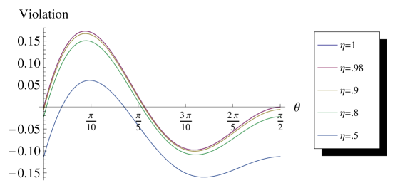
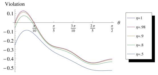
Figures 2 and 3 show the violation of Mermin’s inequality, which is defined as the difference of the right-hand and left-hand sides of Eq. (8), for different efficiencies η𝜂\eta at fixed spin s𝑠s and OPO coefficient r𝑟r. The inequality is violated when the “Violation” is positive in Figs. 2 & 3. The efficiencies decrease from the top to the bottom of the plots—higher efficiencies violate over a greater range of angles, and higher spins require higher efficiencies to produce violations.
Refer to caption

Figure 2: Plot of violation versus angle for different efficiencies for the s=1𝑠1s=1 case. Higher values constitute greater violation; negative results can be explained by a local hidden variable model. Decreasing efficiencies produce decreasing violation. Here, r=0.5𝑟0.5r=0.5.

Refer to caption

Figure 3: Plot of violation versus angle for different efficiencies for the s=2𝑠2s=2 (four photon) case. The results are much the same as in Fig. 5, except the magnitude of violation is lower. Note that there is also a smaller angular range of violation and a greater sensitivity to inefficiencies. Again, r=0.5𝑟0.5r=0.5.

Unsurprisingly, a lower efficiency η𝜂\eta results in considerably reduced violation margins for Mermin’s inequality; as detailed below, violation also decreases with an increase in either the squeezing parameter r𝑟r or the spin s𝑠s. Additionally, the optimal angle for violation appears to shift very slightly as the efficiency decreases.

It’s also important to recall that the situation considered here is perfectly symmetric. All of the detectors have equal efficiency, and the choice of optimal angle θ𝜃\theta (defined by Mermin Mermin1980 ) depends crucially on the equivalence of the two detectors: the otherwise independent detector angles α𝛼\alpha and β𝛽\beta are identical in this model. Further optimizing the violation of Mermin’s inequality over the (really four-dimensional) parameter space of the angles might yield better results for a particular choice of experimental conditions. In the results that follow, however, we only evaluated the inequality at the optimal angle for perfect detection. Thus, the violations we predicted here are, at worst, lower bounds for actual violations.

IV.2 Influence of decoherence on violation for different spins s𝑠s

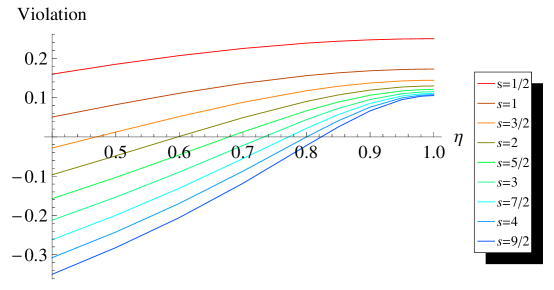
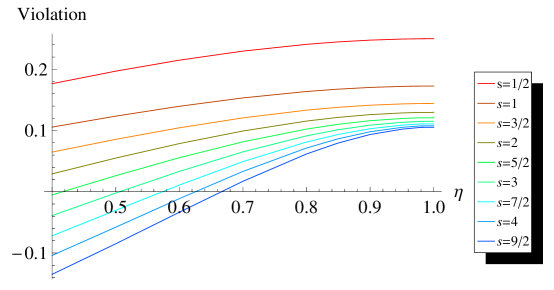
After choosing to evaluate these results at the optimal angles for η=1𝜂1\eta=1, we can examine the effect of inefficiencies more directly by plotting the violation against the efficiency, for r=0.4𝑟0.4r=0.4, Fig. 4, and r=0.2𝑟0.2r=0.2, Fig. 5. These plots are constructed by taking a single point (the maximum in the case of perfect efficiency, near the maximum for lower efficiencies) and combining these points in a plot of violation vs. η𝜂\eta. Different lines on the same plot represent, from top to bottom, different spins from s=1/2𝑠12s={1}/{2} to s=9/2𝑠92s={9}/{2} in steps of 1/212{1}/{2}.

Refer to caption

Figure 4: Plot of violation versus efficiency for different spins s𝑠s. Again, higher values constitute greater violation. Decreasing efficiencies produce decreasing violation, and lower spins violate more strongly than higher spins. Here, r=0.4𝑟0.4r=0.4.

Refer to caption

Figure 5: The same plot as Fig. 4 for r=0.2𝑟0.2r=0.2. Note that the general trends are the same, but violation is stronger. Generally, higher values for r𝑟r give lower violation for η<1𝜂1\eta<1 and vice versa.

As Figs. 4 & 5 show, as the efficiency decreases, all but the lowest spins fail to violate the inequality; the higher the spins, the more deleterious the effect of inefficiency on violation. In Fig. 5, though, all spins tend to violate more strongly than in Fig. 4, especially at low efficiencies. This trend is general—the lower the squeezing parameter r𝑟r, the less effect inefficiency seems to have on violating the inequality.

IV.3 Joint influences of decoherence and squeezing

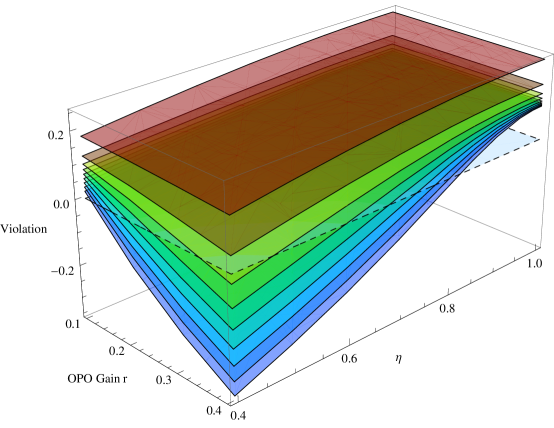
Many of our results can be summarized in the plot of Fig. 6, which again shows the dependence of the violation of Mermin’s inequality on r𝑟r and η𝜂\eta. Note that Figs. 4 & 5 are cross-sections of the Fig. 6 at constant r𝑟r, and that Figs. 2 & 3 have their maxima represented as single points on Fig. 6. Crucially, violations of Mermin’s inequality are predicted for all of these spins under a range of experimentally attainable conditions.
Refer to caption

Figure 6: This plot compares the effect of both squeezing r𝑟r and efficiency η𝜂\eta on the extent of violation. The nine surfaces show the predicted violation for the nine different spins. The top surface is that for s=12𝑠12s=\frac{1}{2}. The next surface is that for s=1𝑠1s=1, and so on, through s=9/2𝑠92s={9}/{2}. Note that the surfaces are labeled with the same color scheme as in Fig. 5 and Fig. 4—these two plots are just the cross sections through the two planes r=0.2𝑟0.2r=0.2 and r=0.4𝑟0.4r=0.4 in this figure. As a reference, a plane is also plotted at zero violation.

There are several trends in these data. First, the extent of violation of the inequality decreases monotonically as the detection efficiency decreases. This was expected. The extent of the decrease, however, depends both on the amount of squeezing and on the total spin itself. On the one hand, low spins almost always violate under the range of conditions plotted here, and have little dependence on either parameter (η𝜂\eta or r𝑟r). Higher spin systems violate less strongly—even in the ideal case of perfect efficiency—and the extent of violation decreases much more rapidly with η𝜂\eta than for lower spin systems. That exacerbated sensitivity of high-spin quantum systems to decoherence is not too surprising either. However, it is important to mention here that several inequalities since Mermin’s time make violation more robust by remedying one or more of these issues. Garg and Mermin later produced an inequality whose angular range of violation does not decrease with increasing spin Garg1982 , and more recent work has produced simple inequalities that are violated even for arbitrarily large spin Peres1992 ; Kaszlikowski2002 ; Collins2002 approaching the maximum possible violation for a 2×2×d22𝑑2\times 2\times d Bell-type experiment Landau1987 ; Durt2001 ; Cirelson1980 . The CGLMP inequality Collins2002 in particular, produces large violations even for large spins and also appears to be resistant to noise in the form of Werner states. We’ve begun exploring the CGLMP inequality in our optical framework, but the form of the inequality makes incorporating loss more computationally intensive than in Mermin’s 1980 inequality. In future work, we plan to address the optical realization of these newer high-spin inequalities.

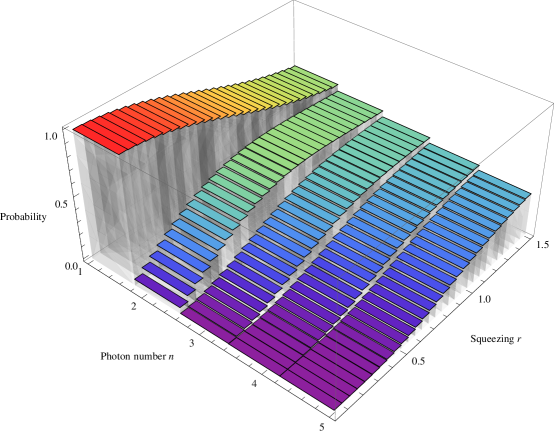
Finally, we see from Fig. 6 that a given spin s𝑠s produced by a strongly squeezed source is much more sensitive to decoherence than the same spin s𝑠s produced by a weakly squeezed source. In the case of perfect detectors, the amount of squeezing doesn’t affect the extent of the violations, but a weakly squeezed state actually produces greater violations than a highly squeezed state if the efficiency is low. This is a much less intuitive result if we associate a more highly squeezed state with less classical behavior, and thus expect a more highly squeezed state to produce greater violations. Our result can be simply explained by the fact that the photon-number distribution of the output fields depends strongly on the squeezing parameter: in EPR states as produced by the OPO, the probability amplitude of a given Fock state is τs,r=(tanhr)n/coshrsubscript𝜏𝑠𝑟superscript𝑟𝑛𝑟\tau_{s,r}=(\tanh r)^{n}/\cosh r , which in both limits goes as a decaying exponential in r𝑟r. So, if the OPO is barely squeezing, the probability for generating a total photon number, or spin state s𝑠s, is much larger than the probability of generating even the next larger spin, whereas, as r𝑟r increases, all of the photon-number states become equally probable, as displayed in Fig. 7.
Refer to caption

Figure 7: Plot of the relative probability of producing a certain photon number in a Fock state as a function of the squeezing r𝑟r. As the squeezing increases, generating larger and larger photon number states becomes more and more probable.

Inefficiencies thus effect a sort of “crossover” between the photon-number states, with a strength increasing as the inefficiency increases: the beamsplitters that model losses annihilate photons from the signal field, which reduces the total spin corresponding to that Fock state in the Schwinger representation. Then, because the measured results are partitioned into individual spin-s𝑠s subspaces before checking for violation, the measured distribution of projections in a given subspace depends both on the distribution in that subspace and on the distribution in higher subspaces, because the higher subspaces will couple to the lower subspaces with an interaction strength determined by the beamsplitter reflection coefficient, or inefficiency of the detector. The relative amplitudes of the two subspaces are therefore crucially important: on the one hand, even if there is strong coupling between the two subspaces through an inefficient detector, if the lower spin subspace has a significantly higher associated probability amplitude, then the effect of the higher spin subspace will be negligible, and this is what happens in the low-squeezing case. If, on the other hand, there is high squeezing, then the two spin subspaces have comparable probability amplitudes and there is a large effect if the detectors are inefficient. For imperfect detectors, higher squeezing thus causes many of the same effects as lower efficiency because both cause a lower-spin subspace to have increased coupling to a higher spin subspace.

Nonetheless, it’s important to remember that there is a significant practical difference between increased squeezing and decreased efficiency. Although theoretically, lower squeezing produces higher violations given inefficient detectors, with low squeezing the OPA produces high photon number states much less frequently. So, there’s a tradeoff: low squeezing will produce higher violations than high squeezing in a nonideal detection case, but one will have to wait much longer to see the violations in an experiment. Increasing the efficiency allows for increased squeezing, which is crucially important for violating any high-spin inequality in a reasonable experimental timeframe.

V Conclusion

Our results show that it appears quite feasible to violate Mermin’s high-spin Bell inequality under a range of experimentally viable conditions. After converting the photon number distribution produced by an optical parametric oscillator from the Fock basis to the spin basis, we find that the state could be written as combination of singlet states typically used to violate Bell-type inequalities. Incorporating inefficiencies into our probabilities by considering the effect of loss through beamsplitters allows us to determine the effect of actual experimental parameters on the outcome of our tests. In particular, we find that Mermin’s inequality is violated for s=1/2𝑠12s={1}/{2} to s=9/2𝑠92s={9}/{2} under a wide range of experimentally realizable efficiencies and squeezing parameters.

In the future, we hope to build on these results by performing an experimental violation of these inequalities using the setup described previously. We hope also to examine other high-dimensional inequalities such as that of Collins, Gisin, Linden, Massar, and PopescuCollins2002 which—though more computationally intensive in this framework—may offer greater violations and increased resistance to experimental imperfections like loss and noise.

This work was supported by NSF grants PHY-0960047 and PHY-0855632, and by the FINESSE program of Raytheon BBN, under the DARPA “Information in a Photon” program. RE was partially supported by an Echols Scholar Ingrassia Research grant at the University of Virginia.

References

  • (1) J. S. Bell, “On the Einstein-Podolsky-Rosen paradox,” Physics 1, 195 (1964).
  • (2) N. D. Mermin, “Quantum mechanics vs local realism near the classical limit: A Bell inequality for spin s𝑠s,” Phys. Rev. D 22, 356 (1980).
  • (3) D. Collins, N. Gisin, N. Linden, S. Massar, and S. Popescu, “Bell Inequalities for Arbitrarily High-Dimensional Systems,” Phys. Rev. Lett. 88, 040404 (2002).
  • (4) N. D. Mermin, “From Cbits to Qbits: Teaching computer scientists quantum mechanics,” American Journal of Physics 71, 23 (2003).
  • (5) A. Aspect, P. Grangier, and G. Roger, “Experimental Realization of Einstein-Podolsky-Rosen-Bohm Gedankenexperiment: A New Violation of Bell’s Inequalities,” Phys. Rev. Lett. 49, 91 (1982).
  • (6) A. Aspect, J. Dalibard, and G. Roger, “Experimental Test of Bell’s Inequalities Using Time- Varying Analyzers,” Phys. Rev. Lett. 49, 1804 (1982).
  • (7) G. Weihs, T. Jennewein, C. Simon, H. Weinfurter, and A. Zeilinger, “Violation of Bell’s Inequality under Strict Einstein Locality Conditions,” Phys. Rev. Lett. 81, 5039 (1998).
  • (8) M. A. Rowe, D. Kielpinski, V. Meyer, C. A. Sackett, W. M. Itano, C. Monroe, and D. J. Wineland, “Experimental violation of a Bell’s inequality with efficient detection,” Nature 409, 791 (2001).
  • (9) T. Scheidl et al., “Violation of local realism with freedom of choice,” PNAS 107, 19708 (2010).
  • (10) J. C. Howell, A. Lamas-Linares, and D. Bouwmeester, “Experimental Violation of a Spin-1 Bell Inequality Using Maximally Entangled Four-Photon States,” Phys. Rev. Lett. 88, 030401 (2002).
  • (11) P. D. Drummond, “Violations of Bell’s Inequality in Cooperative States,” Phys. Rev. Lett. 50, 1407 (1983).
  • (12) M. D. Reid, W. J. Munro, and F. De Martini, “Violation of multiparticle Bell inequalities for low- and high-flux parametric amplification using both vacuum and entangled input states,” Phys. Rev. A 66, 033801 (2002).
  • (13) C. C. Gerry and J. Albert, “Finite violations of a Bell inequality for high spin: An optical realization,” Phys. Rev. A 72, 043822 (2005).
  • (14) J. Schwinger, in Quantum theory of angular momentum, L. C. Biedenharn and H. V. Dam, eds., (Academic Press, 1965), Chap. On angular momentum,  pp. 229–279.
  • (15) J. F. Clauser, M. A. Horne, A. Shimony, and R. A. Holt, “Proposed Experiment to Test Local Hidden-Variable Theories,” Phys. Rev. Lett. 23, 880 (1969).
  • (16) A. Peres, Quantum Theory: Concepts and Methods (Springer, 1995).
  • (17) N. Gisin and A. Peres, “Maximal violation of Bell’s inequality for arbitrarily large spin,” Phys. Lett. A 162, 15 (1992).
  • (18) K. Banaszek and K. Wódkiewicz, “Nonlocality of the Einstein-Podolsky-Rosen state in the Wigner representation,” Phys. Rev. A 58, 4345 (1998).
  • (19) D. F. Walls and G. J. Milburn, Quantum Optics (Springer, Berlin, 1994).
  • (20) A. E. Lita, A. J. Miller, and S. W. Nam, “Counting near-infrared single-photons with 95% efficiency,” Opt. Expr. 16, 3032 (2008).
  • (21) T. Kim, O. Pfister, M. J. Holland, J. Noh, and J. L. Hall, “Influence of decorrelation on Heisenberg-limited interferometry using quantum correlated photons,” Phys. Rev. A 57, 4004 (1998).
  • (22) H. P. Yuen and J. H. Shapiro, “Quantum statistics of homodyne and heterodyne detection,” in Coherence and Quantum Optics IV, L. Mandel and E. Wolf, eds., pp. 719–727 (Plenum, New York, 1978).
  • (23) H. P. Yuen and J. H. Shapiro, “Optical Communication with Two-Photon Coherent States- Part III: Quantum Measurements Realizable with Photoemissive Detectors,” IEEE Trans. Inform. Theory 26, 78 (1980).
  • (24) C. Caves, “Quantum-Mechanical Radiation-Pressure Fluctuations in an Interferometer,” Phys. Rev. Lett. 45, 75 (1980).
  • (25) A. Garg and N. D. Mermin, “Bell Inequalities with a Range of Violation that Does Not Diminish as the Spin Becomes Arbitrarily Large,” Phys. Rev. Lett. 49, 901 (1982).
  • (26) A. Peres, “Finite violation of a Bell inequality for arbitrarily large spin,” Phys. Rev. A 46, 4413 (1992).
  • (27) D. Kaszlikowski, L. C. Kwek, J.-L. Chen, M. Żukowski, and C. H. Oh, “Clauser-Horne inequality for three-state systems,” Phys. Rev. A 65, 032118 (2002).
  • (28) L. J. Landau, “On the violation of Bell’s inequality in quantum theory,” Phys. Lett. A 120, 54 (1987).
  • (29) T. Durt, D. Kaszlikowski, and M. Żukowski, “Violations of local realism with quantum systems described by N-dimensional Hilbert spaces up to N=16𝑁16N=16,” Phys. Rev. A 64, 024101 (2001).
  • (30) B. S. Cirel’son, “Quantum generalizations of Bell’s inequality,” Lett. Math. Phys. 4, 93 (1980).