Extracting the Distribution Amplitudes of the ${\bm{\rho}}$ meson from the Color Glass Condensate

Abstract:

We extract the twist-$2$ and twist-$3$ Distribution Amplitudes (DAs) of the $\rho$ meson using the HERA data on diffractive $\rho$ photoproduction. We do so using several Colour Glass Condensate (CGC) inspired and a Regge inspired dipole models. We find that our extracted twist-$2$ DA is not much model dependent and is consistent with QCD Sum Rules and lattice predictions. The extracted twist-$3$ DA is more model dependent but is still consistent with the Sum Rules prediction.

1 Introduction

In previous papers [1, 2], we extracted the light-cone wavefunctions of the $\rho$ meson and the corresponding twist-$2$ Distribution Amplitude (DA) using the precise HERA data [3, 4] on diffractive $\rho$ photoproduction. In reference [1], we found that the extracted twist-$2$ DA, which is sensitive to the longitudinal light-cone wavefunction, is broader than the asymptotic form $z(1-z)$ and agrees very well with QCD Sum Rules predictions. We showed in reference [2] that this conclusion is not much model dependent. On the other hand, we also found that the data prefer a transverse wavefunction with end-point enhancement [1] although the degree of such an enhancement is model dependent [2].

In this paper, we extend our study in two ways. First, we shall repeat our fits using a CGC-inspired dipole model with a more realistic description of saturation effects than the dipole models we used previously [1, 2]. Second, we extend the analysis beyond twist-$2$ by extracting also the twist-$3$ DA which is sensitive to the scalar part of the transverse light-cone wavefunction. We shall then compare our extracted twist-$2$ and $3$ DAs with lattice [5] and QCD Sum Rules predictions [6].

In references [1, 2], we fit the data using models for the dipole cross section which have been previously constrained by $F_{2}$ data and which also give a good description of the diffractive structure function ($F_{2}^{D(3)}$) data [7, 8]. Such models may be called “forward models” since, by the optical theorem, the dipole cross section is equal to the forward dipole-proton elastic scattering amplitude. Such models do account for saturation, but in a way independent of the momentum transfer $t$ or the impact parameter $b$.

More realistic dipole models take into account the $t$ or $b$-dependence of saturation effects and have been proposed in references [9, 10, 11]. Here, we shall use the model by Marquet, Peschanski and Soyez [10] and refer to it as the t-CGC model. Given the limited $Q^{2}\in[0,41]~{}\mbox{GeV}^{2}$ range of the HERA data on diffractive $\rho$ production to which we fit, we do not consider DGLAP evolution [12, 11].

2 Amplitudes and cross-sections

In the dipole model [13, 14], the imaginary part of the amplitude for diffractive $\rho$ production is given by [10]:

$$\Im\mbox{m}\mathcal{A}_{\lambda}(s,t;Q^{2})=\sum_{h,\bar{h}}\int\mathrm{d}^{2}\mathbf{r}\;\mathrm{d}z\;\Psi^{\gamma^{*},\lambda}_{h,\bar{h}}(r,z;Q^{2})\Psi^{\rho,\lambda}_{h,\bar{h}}(r,z)^{*}e^{-iz\mathbf{r}.\mathbf{\Delta}}\mathcal{N}(x,\mathbf{r},\mathbf{\Delta})\;,$$ (1)

where $t=-|\mathbf{\Delta}|^{2}$. $\Psi^{\gamma^{*},\lambda}_{h,\bar{h}}(r,z;Q^{2})$ and $\Psi^{\rho,\lambda}_{h,\bar{h}}(r,z)$ denote the light-cone wavefunctions of the photon and $\rho$-meson respectively while $\mathcal{N}(x,\mathbf{r},\mathbf{\Delta})$ is the dipole-proton scattering amplitude.

We choose the dimensionless variable $x$ carrying the energy dependence of the dipole-proton elastic amplitude $\mathcal{N}(x,\mathbf{r},\mathbf{\Delta})$ to be a modified Bjorken-$x$:

$$x=x_{\mathrm{Bj}}\left(1+\frac{4m_{f}^{2}}{Q^{2}}\right)$$ (2)

with a phenomenological quark mass of $m_{f}=0.14~{}\mbox{GeV}$. This choice coincides with $x_{\mathrm{Bj}}$ at high $Q^{2}$ and replaces the latter at low $Q^{2}$. We should point out that the optimal choice for the dimensionless variable that carries the energy dependence of the dipole-proton amplitude remains an open and interesting problem [15]. For instance, it can be argued that the dipole-proton amplitude should not depend at all on the photon’s virtuality [16, 17].

Assuming that $\mathcal{N}(x,\mathbf{r},\mathbf{\Delta})=\mathcal{N}(x,r,\mathbf{\Delta})$, the angular integration can be carried out giving

$$\Im\mbox{m}\mathcal{A}_{\lambda}(s,t;Q^{2})=2\pi\sum_{h,\bar{h}}\int\mathrm{d}r\;\mathrm{d}z\;rJ_{0}(rz\Delta)\;\Psi^{\gamma^{*},\lambda}_{h,\bar{h}}(r,z;Q^{2})\Psi^{\rho,\lambda}_{h,\bar{h}}(r,z)^{*}\mathcal{N}(x,r,\mathbf{\Delta})\;.$$ (3)

Note that by setting $t=0$ in equation (1), we recover the forward amplitude used in references [1, 2], i.e.

$$\left.\Im\mbox{m}\,\mathcal{A}_{\lambda}(s,t;Q^{2})\right|_{t=0}=s\sum_{h,\bar{h}}\int\mathrm{d}^{2}{\mathbf{r}}\;\mathrm{d}z\;\Psi^{\gamma,\lambda}_{h,\bar{h}}(r,z;Q^{2})\hat{\sigma}(x,r)\Psi^{\rho,\lambda}_{h,\bar{h}}(r,z)^{*}$$ (4)

where we have introduced the dipole cross-section

$$\hat{\sigma}(x,r)\equiv\frac{\mathcal{N}(x,r,\mathbf{0})}{s}=\frac{1}{s}\int\mathrm{d}^{2}\mathbf{b}\;\tilde{\mathcal{N}}(x,r,\mathbf{b})\;.$$ (5)

This means that the dipole cross-section is independent of the impact parameter and that any modelling of saturation at the level of this cross-section is necessarily $t$-independent. Nevertheless, the dipole cross-section can be extracted using the high quality $F_{2}$ data and can then be used to predict the imaginary part of the forward amplitude for diffractive $\rho$ production and thus the forward differential cross-section:

$$\left.\frac{\mathrm{d}\sigma_{\lambda}}{\mathrm{d}t}\right|_{t=0}=\frac{1}{16\pi}(\Im\mathrm{m}\mathcal{A}_{\lambda}(s,0))^{2}\;(1+\beta_{\lambda}(0)^{2})~{},$$ (6)

where $\beta_{\lambda}(0)$ is the ratio of real to imaginary parts of the forward amplitude and is computed as in reference [1]. The $t$-dependence can be restored as suggested by experiment [3]:

$$\frac{d\sigma_{\lambda}}{dt}=\left.\frac{d\sigma_{\lambda}}{dt}\right|_{t=0}\times\exp(-B|t|)$$ (7)

where

$$B=N\left(14.0\left(\frac{1~{}\mathrm{GeV}^{2}}{Q^{2}+M_{\rho}^{2}}\right)^{0.2}+1\right)$$ (8)

with $N=0.55$ GeV^-2. Note that in doing this, we are assuming that it is a reasonable approximation to consider the ratio of real to imaginary part of the the amplitude to be independent of $t$, i.e. $\beta_{\lambda}(0)\approx\beta_{\lambda}(t)$.

In the non-forward case,

$$\frac{d\sigma_{\lambda}}{dt}=\frac{1}{16\pi}(\Im\mathrm{m}\mathcal{A}_{\lambda}(s,t))^{2}\;(1+\beta_{\lambda}(t)^{2})~{},$$ (9)

where $\beta_{\lambda}(t)$ is now the ratio of real to imaginary parts of the non-forward amplitude and is computed in the same way as $\beta_{\lambda}(0)$. This differential cross-section is measured at HERA [3, 4].

The total cross-section, which is also measured at HERA, is obtained by integrating either (7) or equation (9) over $t$. In the former case, this integration is trivially performed analytically for each polarisation and the total cross-section is taken to be $\sigma=\sigma_{L}+\epsilon\sigma_{T}$. In the non-forward case, we integrate equation (9) numerically over $t$ to obtain the total cross-section.

3 Dipole models

In principle, the dipole-proton scattering amplitude $\tilde{\mathcal{N}}(x,r,b)$ can be obtained by solving the Balitsky-Kovchegov (BK) equation [18, 19, 20] which itself can be derived within the Colour Glass Condensate (CGC) formalism [21, 22, 23, 24, 25]. However, work is still in progress to implement in a satisfactory way the impact-parameter dependence in the BK equation [26]. On the other hand, an approximate solution for the forward dipole-proton amplitude has been proposed several years ago by Iancu, Itakura and Munier [27]:

$$\mathcal{N}(rQ_{s},x,0) = {\cal N}_{0}\left(\frac{rQ_{s}}{2}\right)^{2\left[\gamma_{s}+\frac{\ln(2/rQ_{s})}{\kappa\lambda\ln(1/x)}\right]}\hskip 28.45274pt\mathrm{for}\hskip 28.45274ptrQ_{s}\leq 2$$ (10)

$$= \{1-\exp[-a\ln^{2}(brQ_{s})]\}\hskip 28.45274pt\mathrm{for}\hskip 28.45274ptrQ_{s}>2~{},$$

where the saturation scale $Q_{s}\equiv(x_{0}/x)^{\lambda/2}$ GeV. The dipole cross-section is then given by $\hat{\sigma}(rQ_{s},x)=\sigma_{0}\mathcal{N}(rQ_{s},x,0)$. In reference [27], the anomalous dimension $\gamma_{s}$ was fixed to its LO BFKL value of $0.63$ while the free parameters $\sigma_{0}$, $x_{0}$ and $\lambda$ are determined by fitting to the $F_{2}$ data, without a charm contribution. When charm was included in reference [11], it was found that the saturation scale decreases dramatically. We used this fit in reference [2] where we referred to it as CGC[$0.63$]. However, Soyez later showed that letting the anomalous dimension $\gamma_{s}$ vary freely also gives a good $F_{2}$ fit with no significant decrease in the saturation scale [28]. The resulting value of $\gamma_{s}$ is $0.74$, close to the value obtained with the RG-improved NLO BFKL kernel  [28]. Kowalski and Watt confirmed the Soyez fit in reference [9] and we used their fitted parameters in reference [2] where we referred to it as the CGC[$0.74$] fit. This model has been extended by Marquet, Peschanski and Soyez to include a $t$-dependence in the saturation scale resulting in what we now refer to as the t-CGC model. In the t-CGC model [10],

$$\mathcal{N}(rQ_{s}(t),\mathbf{r},t)=\mathcal{N}(rQ_{s}(t),\mathbf{r},0)\times\exp(-B|t|)$$ (11)

where

$$Q_{s}(t)=(x_{0}/x)^{\lambda/2}(1+c\sqrt{|t|})\;.$$ (12)

The t-CGC model has two additional free parameters ($c$ and $B$) compared to its forward counterpart, i.e. CGC[$0.74$]. In reference [10], these parameters were fixed by a global fit to a subset of the vector meson ($\rho$,$\phi$ and $J/\Psi$) production data including the earlier $\rho$ data from H1 [29]. The authors of reference [10] selected those data that were were not too sensitive to the precise shape of the meson wavefunction and did not include the $\sigma_{L}/\sigma_{T}$ data. As shown in table 1, all other parameters, including the anomalous dimension $\gamma_{s}$, have the same values as in the forward case. This ensures that the quality of the $F_{2}$ fit is unaltered in the t-CGC model compared to that with the CGC[$0.74$] model.

The CGC models are based on perturbative QCD and, for that reason, the original fits to $F_{2}$ were in the range $Q^{2}\in[0.25,45]~{}\mbox{GeV}^{2}$, thereby excluding the available data in the low $Q^{2}$ range, $Q^{2}\in[0.045,0.20]~{}\mbox{GeV}^{2}$, a kinematic region where perturbation theory is not reliable [9]. In these fits the light quark mass was neglected compared to $Q^{2}$ so that the dipole-proton amplitude is evaluated at $x=x_{\mathrm{Bj}}$ when computing the light quark contribution to the structure function [9]. By using equation (2), we shall dare to extrapolate the use of the CGC dipole models to low $Q^{2}$, including $Q^{2}=0$. In order to legitimate such a procedure, we verify that these models still describe the $F_{2}$ data in the extended range $Q^{2}\in[0.045,45]~{}\mbox{GeV}^{2}$, where the numerical difference between $x$ given by (2) and $x_{\mathrm{Bj}}$ can be significant. The resulting $\chi^{2}/\mbox{d.p}$ values thus obtained are shown in the last column of table 1. They indicate that it is reasonable to extrapolate the use of the CGC models to low $Q^{2}$, together with the modified Bjorken-$x$ given by equation (2).

Finally, we shall also use the Regge-inspired FSSat dipole model [30], for which the original $F_{2}$ fits were inclusive of the low $Q^{2}$ data, i.e. with $Q^{2}\in[0.045,45]~{}\mbox{GeV}^{2}$. This model falls in the category of forward models, like CGC[$0.63$] and CGC[$0.74$], where saturation effects are assumed to be independent of momemtum transfer.

Note that we are using here simple phenomenological parametrizations for the dipole-proton scattering amplitude subject to the requirement that they fit the $F_{2}$ data. Such simple parametrizations are convenient for extracting the meson light-cone wavefunction. We do not consider here the more sophisticated solutions to the BK equation with running coupling [31, 32] or the dipole cascade model [33].

CGC $F_{2}$ fits

$$\begin{array}[c]{|c|c|c|c|c|c|c|c|c|}\hline\cr\mbox{Model}&\gamma_{s}&x_{0}&\lambda&\sigma_{0}[\mbox{mb}]&B~{}\mbox{GeV}^{-2}&c~{}\mbox{GeV}^{-1}&\chi^{2}/133~{}\mbox{d.p}&\chi^{2}/156~{}\mbox{d.p}\\ \hline\cr\mbox{CGC[$0.63$]}&0.63~{}(\mbox{fixed})&1.09\times 10^{-7}&0.170&37.4&-&-&119/133&135/156\\ \hline\cr\mbox{CGC[$0.74$]}&0.74&1.63\times 10^{-5}&0.216&27.4&-&-&113/133&145/156\\ \hline\cr\mbox{t-CGC}&0.74&1.63\times 10^{-5}&0.216&27.4&3.754&4.077&113/133&145/156\\ \hline\cr\end{array}$$

Table 1: The fitted parameters of the CGC dipole models obtained from fits to $F_{2}$ with $Q^{2}\in[0.25,45]~{}\mbox{GeV}^{2}$ and $x_{\mathrm{Bj}}\leq 0.01$. For each model, the first $\chi^{2}/\mbox{d.p}$ value is obtained when the model is fitted to $F_{2}$ data with $Q^{2}\in[0.25,45]~{}\mbox{GeV}^{2}$. The second $\chi^{2}/\mbox{d.p}$ value is a prediction of the fitted model when tested in the extended range $Q^{2}\in[0.045,45]~{}\mbox{GeV}^{2}$.

All the forward models we consider also give a good description of the diffractive structure function ($F_{2}^{D(3)}$) data [8, 7]. The non forward models have been applied to describe a number of processes [34, 35] including (in the approach of reference [9]) inclusive hadron production, for which the first LHC data are now available [36, 37].

4 Light-cone wavefunctions

By analogy with the photon’s light-cone wavefunction, the $\rho$ meson wavefunction can be factorised into a spinor and scalar part [38]. In momentum space,

$$\Psi^{\rho,\lambda}_{h,\bar{h}}(z,\mathbf{k})=\sqrt{\frac{N_{c}}{4\pi}}S_{h,\bar{h}}^{\rho,\lambda}(z,\mathbf{k})\phi_{\lambda}(z,\mathbf{k})$$ (13)

where

$$S_{h,\bar{h}}^{\rho,\lambda}(z,\mathbf{k})=\frac{\bar{u}_{h}(zP^{+},-\mathbf{k})}{\sqrt{z}}e^{\lambda}.\gamma\frac{v_{\bar{h}}((1-z)P^{+},\mathbf{k})}{\sqrt{(1-z)}}$$ (14)

where $P^{+}$ is the “plus” component of the $4$-momentum of the meson given by

$$P^{\mu}=\left(P^{+},\frac{M_{\rho}^{2}}{2P^{+}},0_{\perp}\right)\;.$$ (15)

Using the longitudinal polarisation vector

$$e^{L}=\left(\frac{P^{+}}{M_{\rho}},-\frac{M_{\rho}}{2P^{+}},0_{\perp}\right)$$ (16)

we can write

$$S_{h,\bar{h}}^{\rho,L}(z,\mathbf{k})=[S_{h,\bar{h}}^{\rho,L}(z,\mathbf{k})]_{+}+[S_{h,\bar{h}}^{\rho,L}(z,\mathbf{k})]_{-}$$ (17)

where [39]

$$[S_{h,\bar{h}}^{\rho,L}(z,\mathbf{k})]_{+}=-\frac{M_{\rho}}{2P^{+}}\left[\frac{\bar{u}_{h}}{\sqrt{z}}\gamma^{+}\frac{v_{\bar{h}}}{\sqrt{1-z}}\right]=-M_{\rho}\delta_{h,-\bar{h}}$$ (18)

and

$$[S_{h,\bar{h}}^{\rho,L}(z,\mathbf{k})]_{-}=\frac{P^{+}}{M_{\rho}}\left[\frac{\bar{u}_{h}}{\sqrt{z}}\gamma^{-}\frac{v_{\bar{h}}}{\sqrt{(1-z)}}\right]=-\frac{m_{f}^{2}+\mathbf{k}^{2}}{z(1-z)M_{\rho}}\delta_{h,-\bar{h}}$$ (19)

so that

$$S_{h,\bar{h}}^{\rho,L}(z,\mathbf{k})=-\frac{1}{M_{\rho}z(1-z)}\left[z(1-z)M^{2}_{\rho}+m_{f}^{2}+\mathbf{k}^{2}\right]\delta_{h,-\bar{h}}\;.$$ (20)

To evaluate the transverse spinor wavefunction, we use the polarisation vector

$$e^{T}=\frac{1}{\sqrt{2}}\left(0,0,\mathbf{e_{\perp}^{\pm}}\right)~{}\hskip 28.45274pt~{}\mbox{with}\hskip 28.45274pt\mathbf{e_{\perp}^{\pm}}=(1,\pm i)$$ (21)

to obtain [39]

$$S_{h,\bar{h}}^{\rho,T(\pm)}(z,\mathbf{k})=\pm\frac{\sqrt{2}}{z(1-z)}\{[z\delta_{h\pm,\bar{h}\mp}-(1-z)]\delta_{h\mp,\bar{h}\pm}ke^{\pm i\theta_{k}}+m_{f}\delta_{h\pm,\bar{h}\pm}\}$$ (22)

where we have used the polar representation of the transverse momentum, i.e. $\mathbf{k}=ke^{i\theta_{k}}$.

Taking the two-dimensional Fourier transforms of equation (13), we obtain the $r$-space light-cone wavefunctions [38]:

$$\Psi^{\rho,L}_{h,\bar{h}}(r,z)=-\sqrt{\frac{N_{c}}{4\pi}}\delta_{h,-\bar{h}}\frac{1}{M_{\rho}z(1-z)}[z(1-z)M^{2}_{\rho}+m_{f}^{2}-\nabla_{r}^{2}]\phi_{L}(r,z)$$ (23)

where $\nabla_{r}^{2}\equiv\frac{1}{r}\partial_{r}+\partial^{2}_{r}$, and

$$\Psi^{\rho,T(\gamma=\pm)}_{h,\bar{h}}(r,z)=\pm\sqrt{\frac{N_{c}}{4\pi}}\frac{\sqrt{2}}{z(1-z)}[ie^{\pm i\theta_{r}}(z\delta_{h\pm,\bar{h}\mp}-(1-z)\delta_{h\mp,\bar{h}\pm})\partial_{r}+m_{f}\delta_{h\pm,\bar{h}\pm}]\phi_{T}(r,z).$$ (24)

Previous work [38, 10, 9, 33] has argued that a reasonable assumption for the scalar part of the light-cone wavefunction for the $\rho$ is of the form

$$\phi^{{\mathrm{BG}}}_{\lambda}(r,z) = \mathcal{N}_{\lambda}\;4[z(1-z)]^{b_{\lambda}}\sqrt{2\pi R_{\lambda}^{2}}\;\exp\left(\frac{m_{f}^{2}R_{\lambda}^{2}}{2}\right)\exp\left(-\frac{m_{f}^{2}R_{\lambda}^{2}}{8[z(1-z)]^{b_{\lambda}}}\right)$$

$$\times\exp\left(-\frac{2[z(1-z)]^{b_{\lambda}}r^{2}}{R_{\lambda}^{2}}\right)\;,$$

which is referred to as the “Boosted Gaussian” (BG) wavefunction. These light-cone wavefunctions are normalised:

$$\int\mathrm{d}^{2}{\mathbf{r}}\mathrm{d}z|\Psi^{\rho,\lambda}(r,z)|^{2}=1\;,$$ (26)

where we have defined

$$|\Psi^{\rho,\lambda}(r,z)|^{2}\equiv\sum_{h,\bar{h}}|\Psi^{\rho,\lambda}_{h,\bar{h}}(r,z)|^{2}\;.$$ (27)

This normalisation condition embodies the assumption that the $\rho$ consists of the leading $q\bar{q}$ Fock state only. In addition, the longitudinal light-cone wavefunction is subject to the leptonic decay width constraint [38]:

$$\sqrt{2}f_{\rho}M_{\rho}=\frac{N_{c}}{\pi}\int_{0}^{1}\mathrm{d}z\left.[z(1-z)M^{2}_{\rho}+m_{f}^{2}-\nabla_{r}^{2}]\frac{\phi_{L}(r,z)}{z(1-z)}\right|_{r=0}\;,$$ (28)

where the decay constant $f_{\rho}$ is simply related to the experimentally measured electronic decay width $\Gamma_{\rho\rightarrow e^{+}e^{-}}$ of the $\rho$ [1].

5 Fitting the HERA data

In the original BG wavefunction, $b_{L}=b_{T}=1$ and $R_{L}^{2}=R_{T}^{2}=12.9~{}\mbox{GeV}^{-2}$ so that the leptonic decay width and the normalisation constraints are satisfied. However, when this BG wavefunction is used in conjunction with either the FSSat or any of the CGC models, none of them is able to give a good quantitative agreement with the current HERA data. This situation is considerably improved by letting $R_{\lambda}$ and $b_{\lambda}$ vary freely and this enhances end-point contributions. We also investigate the requirement for additional end-point enhancement in the transverse wavefunction by using a scalar wavefunction of the form

$$\phi_{T}(r,z)=\phi^{{\mathrm{BG}}}_{T}(r,z)\times[1+c_{T}\xi^{2}+d_{T}\xi^{4}]$$ (29)

where $\xi=2z-1$.

We fit to the same data set as in reference [1], i.e. to total cross-section data, the ratio of longitudinal to transverse cross-section data and the decay constant datum for the longitudinally polarised meson, i.e. to a total of $76$ data points. For the non-forward models, we also include the differential cross-section data with $|t|\leq 0.5~{}\mbox{GeV}^{2}$ ($46$ data points) resulting in a total of $122$ data points. As in reference [1], we rescale the overall normalisation of the data down by $5\%$ which is consistent with the experimental uncertainty.

Note that for the non-forward t-CGC model, we make use of the current data on the differential cross-section to refit the parameters controlling the $t$-dependence. This means that there are $2$ additional free parameters, $B$ and $c$, compared to the forward FSSat, CGC[$0.63$] and CGC[$0.74$] fits.

Our best fit parameters and resulting $\chi^{2}/\mbox{d.o.f}$ are given in table 2. For the t-CGC model, we find two successful fits which we refer to as t-CGC and t-CGC(alt.). We choose to record the alternative t-CGC fit because we extract from it a qualitatively different shape for the transverse wavefunction: the parameters $c_{T}$ and $d_{T}$ go negative in this fit.

We note that our fitted values for the parameters controlling the $t$-dependence are $B=3.159(3.229)~{}\mbox{GeV}^{-2}$ and $c=1.146(1.262)~{}\mbox{GeV}^{-2}$, where the number in brackets corresponds to the alternative t-CGC fit. The values for $c$ are lower than that obtained in reference  [10] and which we quote in table 1.

Our fits to the HERA data are shown in figures 3 and 4 for the total cross-section, in figure 5 for the $\sigma_{L}/\sigma_{T}$ ratio. In figures 6 and 7 we show the t-CGC fit to the differential cross-section data as well as the predictions of the forward models FSSat, CGC[$0.63$] and CGC[$0.74$].

Best fits for the meson wavefunction

$$\begin{array}[c]{|c|c|c|c|c|c|c|c|c|}\hline\cr\mbox{Reference}&\mbox{Model}&R_{L}^{2}&R_{T}^{2}&b_{L}&b_{T}&c_{T}&d_{T}&\chi^{2}/\mbox{d.o.f}\\ \hline\cr\mbox{\cite[cite]{[\@@bibref{}{Forshaw:2010py,Boer:2011fh}{}{}]}}&\mbox{FSSat}&26.76&27.52&0.5665&0.7468&0.3317&1.310&68/70\\ \hline\cr\mbox{\cite[cite]{[\@@bibref{}{Boer:2011fh}{}{}]}}&\mbox{CGC}[0.63]&27.31&31.92&0.5522&0.7289&1.6927&2.1457&67/70\\ \hline\cr\mbox{\cite[cite]{[\@@bibref{}{Boer:2011fh}{}{}]}}&\mbox{CGC}[0.74]&26.67&21.30&0.5697&0.7929&0&0&64/72\\ \hline\cr\mbox{This paper}&\mbox{t-CGC}&29.63&21.64&0.5018&0.7396&0&0&114/116(72/75)\\ \hline\cr\mbox{This paper}&\mbox{t-CGC (alt.)}&29.68&20.96&0.5004&0.7314&-0.1601&-0.1656&112/114(70/75)\\ \hline\cr\end{array}$$

Table 2: Best fit wavefunction parameters and resulting $\chi^{2}/\mbox{d.o.f}$ obtained with each dipole model. For the non-forward t-CGC model, the partial $\chi^{2}/\mbox{d.p}$ for the total cross-section and ratio data is given in brackets.

In figures 1 and 2, we show the extracted light-cone wavefunctions squared, as defined by equation (27), and evaluated at $r=0$. Figure 1 confirms that the longitudinal wavefunction is not much model-dependent. On the other hand, figure 2 shows that the data allow for a wide range of end-point enhancement in the transverse wavefunction.

Additional theoretical constraints on the $\rho$ light-cone wavefunction can be obtained from QCD Sum Rules and lattice QCD. More precisely, these non-perturbative methods can predict the moments of the DA at a low non-perturbative scale. In order to use these constraints we must first establish the relationship between the DA and the light-cone wavefunction. We shall then be in a position to compare the DA predicted by each of our extracted wavefunctions with QCD Sum Rules and lattice predictions.

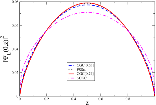
Figure 1: The longitudinal light-cone wavefunction squared evaluated at $r=0$. Solid: CGC[$0.74$], Dotted: FSSat, Dashed: CGC[$0.63$], Dot-dashed: t-CGC. The alternative t-CGC(alt.) fit is indistinguishable from the t-CGC fit.

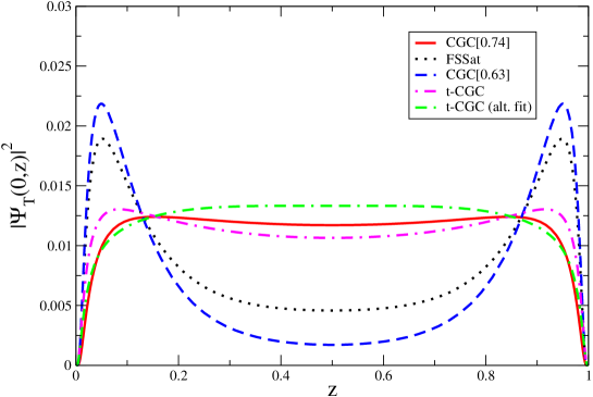
Figure 2: The transverse light-cone wavefunction squared evaluated at $r=0$. Solid: CGC[$0.74$], Dotted: FSSat, Dashed: CGC[$0.63$], Dot-dashed: t-CGC, dash-dash-dotted: t-CGC(alt.).

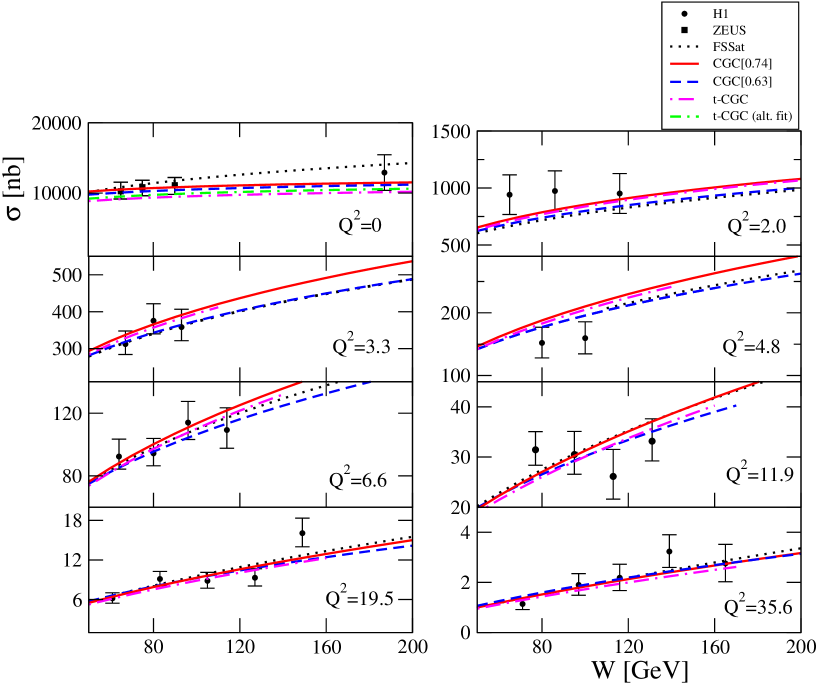
Figure 3: Fits to the HERA cross-section data. Solid: CGC[0.74], dotted: FSSat, dashed: CGC[0.63], dot-dashed: t-CGC. The alternative t-CGC(alt.) fit is only shown at $Q^{2}=0~{}\mbox{GeV}^{2}$ since at higher $Q^{2}$ it is indistinguishable from the t-CGC fit.

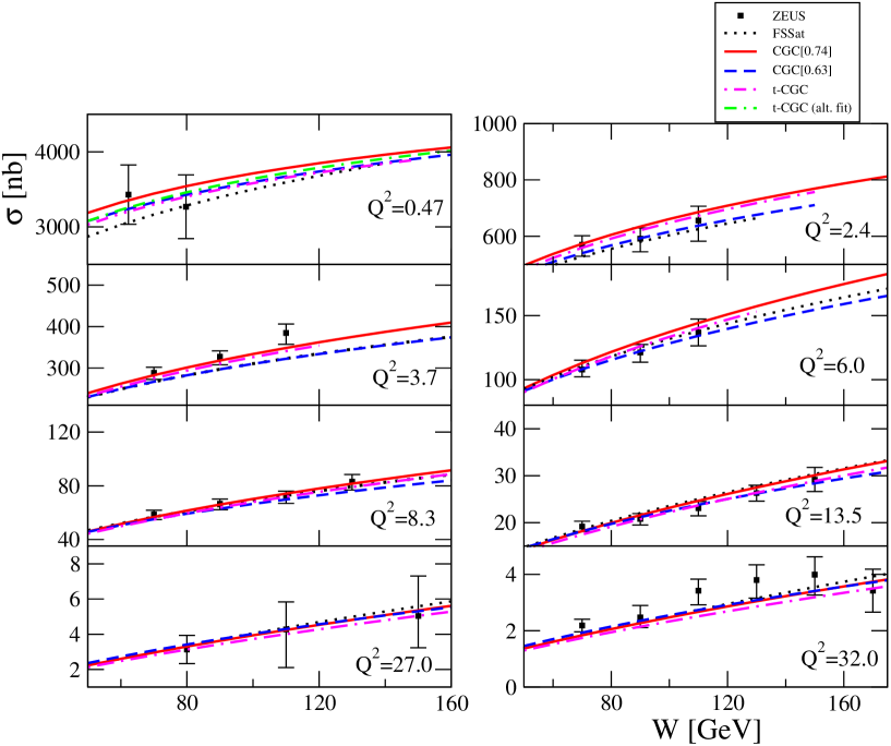
Figure 4: Fits to the ZEUS total cross-section. Solid: CGC[0.74], dotted: FSSat, dashed: CGC[0.63], dot-dashed: t-CGC. The alternative t-CGC fit is only shown at $Q^{2}=0.47~{}\mbox{GeV}^{2}$ since at higher $Q^{2}$ it is indistinguishable from the t-CGC fit.

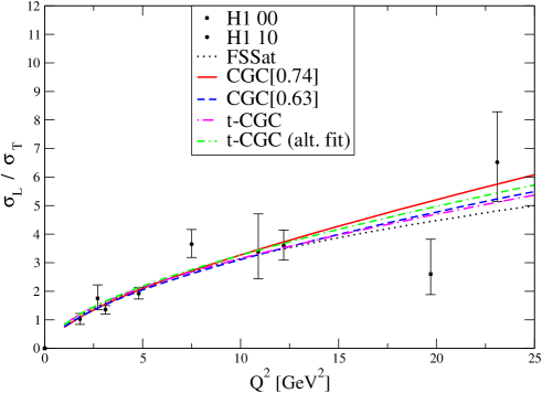
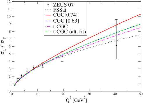
Figure 5: The $\sigma_{L}/\sigma_{T}$ data are at $W=75$ GeV for H1 and $W=90$ GeV for ZEUS. Solid: CGC[0.74], dotted: FSSat, dashed: CGC[0.63], dot-dashed: t-CGC, dash-dash-dotted: t-CGC(alt.).

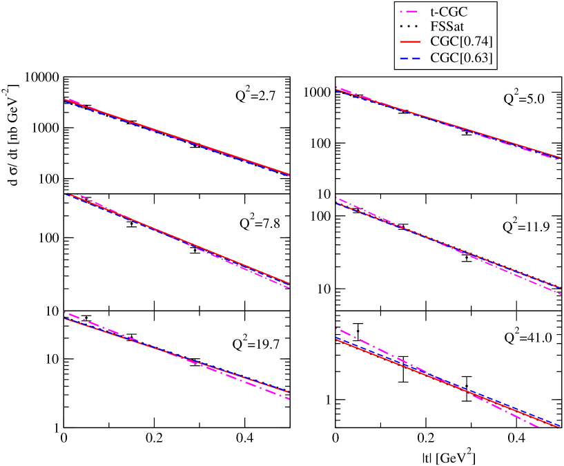
Figure 6: Dot-dashed: t-CGC fit to the differential cross-section data from ZEUS in the range $0\leq|t|\leq 0.5~{}\mbox{GeV}^{2}$. At these values of $Q^{2}$ the alternative t-CGC(alt.) fit is indistinguishable from the t-CGC fit and is not shown here. Also shown are the predictions of the forward models: Solid: CGC[0.74], dotted: FSSat, dashed: CGC[0.63].

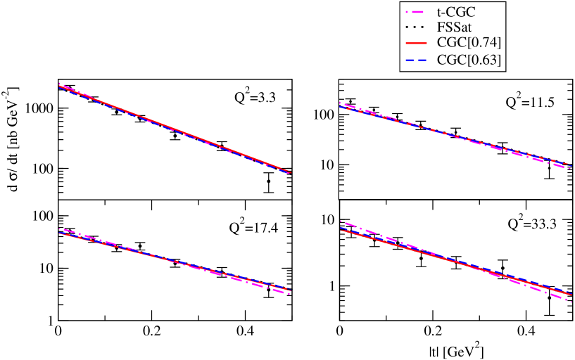
Figure 7: Dot-dashed: t-CGC fit to the differential cross-section data from H1 in the range $0\leq|t|\leq 0.5~{}\mbox{GeV}^{2}$. At these values of $Q^{2}$ the alternative t-CGC(alt.) fit is indistinguishable from the t-CGC fit and is not shown here. Also shown are the predictions of the forward models: Solid: CGC[0.74], dotted: FSSat, dashed: CGC[0.63].

6 Distribution Amplitudes

Light-cone DAs appear in the operator product expansion of vacuum-to-meson transition matrix elements of quark-antiquark non-local gauge invariant operators at light-like separations: [44]

$$\langle 0|\bar{q}(0)[0,x]\gamma^{\mu}q(x)|\rho(P,\lambda)\rangle = \sqrt{2}f_{\rho}M_{\rho}\frac{e_{\lambda}\cdot x}{P\cdot x}\,P^{\mu}\int_{0}^{1}\mathrm{d}u\,e^{-iuP\cdot x}\phi_{\parallel}(u,\mu)$$ (30)

$${}+\left(e_{\lambda}^{\mu}-P^{\mu}\frac{e_{\lambda}\cdot x}{P\cdot x}\right)\sqrt{2}f_{\rho}M_{\rho}\int_{0}^{1}\mathrm{d}u\,e^{-iuP\cdot x}\,g_{\perp}(u,\mu)$$

$${}+\{\cdots\}$$

where $\mu$ is the renormalization scale, $x\cdot x=0$. The gauge link

$$[0,x]=\mbox{\rm Pexp}[ig\!\!\int_{0}^{1}\!\!\mathrm{d}t\,(-x)_{\mu}A^{\mu}((1-t)x)],$$ (31)

ensures the gauge invariance of the matrix elements. According to the classification of Ball and Braun [42, 44], $\phi_{\parallel}$ is twist-$2$ and $g_{\perp}$ is twist-$3$. The $\{\cdots\}$ in equation (30) stand for higher twist contributions [42, 44] which we do not consider here.

The $\mu$-dependent DAs

$$\varphi=\{\phi_{\parallel},g_{\perp}\}$$ (32)

satisfy the following normalisation condition:

$$\int_{0}^{1}\mathrm{d}u\;\varphi(u,\mu)=1\;.$$ (33)

This guarantees that in the local limit $x\rightarrow 0$, (30) becomes

$$\langle 0|\bar{q}(0)\gamma^{\mu}q(0)|\rho(P,\lambda)\rangle=\sqrt{2}f_{\rho}M_{\rho}e^{\mu}_{\lambda}$$ (34)

thereby recovering the definition of the decay constant $f_{\rho}$.

In order to establish a connection between these DAs and the light-cone wavefunctions of the $\rho$, we need to apply the equal light-cone time condition, $x^{+}=0$ and choose the light-cone gauge $A^{+}=0$. We can therefore rewrite equation (30) as

$$\langle 0|\bar{q}(0)\gamma^{\mu}q(0,x^{-},0_{\perp})|\rho(P,\lambda)\rangle = \sqrt{2}f_{\rho}M_{\rho}\frac{e_{\lambda}\cdot x}{P^{+}x^{-}}\,P^{\mu}\int_{0}^{1}\mathrm{d}u\;e^{-iuP^{+}x^{-}}\phi_{\parallel}(u,\mu)$$ (35)

$$+ \sqrt{2}f_{\rho}M_{\rho}\left(e_{\lambda}^{\mu}-P^{\mu}\frac{e_{\lambda}\cdot x}{P^{+}x^{-}}\right)\int_{0}^{1}\mathrm{d}u\;e^{-iuP^{+}x^{-}}g_{\perp}(u,\mu)$$

To isolate $\phi_{\parallel}$, we take $\mu=+$ with $\lambda=L$ in equation (35) and obtain

$$\langle 0|\bar{q}(0)\gamma^{+}q(x^{-})|\rho(P,L)\rangle=\sqrt{2}f_{\rho}P^{+}\int\mathrm{d}u\;e^{-iuP^{+}x^{-}}\phi_{\parallel}(u,\mu)\;.$$ (36)

On the other hand, to isolate $g_{\perp}$, we take the scalar product of equation (35) with the complex conjugate of the meson’s transverse polarization vector to arrive at

$$\langle 0|\bar{q}(0)e_{T}^{*}\cdot\gamma q(x^{-})|\rho(P,T)\rangle=\sqrt{2}f_{\rho}M_{\rho}\int\mathrm{d}u\;e^{-iuP^{+}x^{-}}g_{\perp}(u,\mu)\;.$$ (37)

Taking the Fourier transform of the above matrix elements with respect to the longitudinal light-cone distance $x^{-}$ yields:

$$\phi_{\parallel}(z,\mu)=\frac{1}{\sqrt{2}f_{\rho}}\int\mathrm{d}x^{-}e^{izP^{+}x^{-}}\langle 0|\bar{q}(0)\gamma^{+}q(x^{-})|\rho(P,L)\rangle$$ (38)

and

$$g_{\perp}(z,\mu)=\frac{P^{+}}{\sqrt{2}f_{\rho}M_{\rho}}\int\mathrm{d}x^{-}e^{izP^{+}x^{-}}\langle 0|\bar{q}(0)e^{T*}.\gamma q(x^{-})|\rho(P,T)\rangle\;.$$ (39)

We now wish to express the matrix elements on the right-hand-sides of the above equations (38) and (39) in terms of the meson’s light-cone wavefunction given by equation (13). To do so, we use the Fock expansion

$$|\rho(P,\lambda)\rangle=\sqrt{4\pi N_{c}}\sum_{h,\bar{h}}\int\frac{\mathrm{d}k^{+}\mathrm{d}^{2}\mathbf{k}}{16\pi^{3}\sqrt{k^{+}(P^{+}-k^{+})}}\Psi^{\rho,\lambda}_{h,\bar{h}}(k^{+}/P^{+},\mathbf{k})\hat{b}_{h}^{\dagger}(k^{+},\mathbf{k})\hat{d}_{\bar{h}}^{\dagger}((P^{+}-k^{+}),-\mathbf{k})|0\rangle$$ (40)

and the mode expansion

$$q(0,x^{-},\mathbf{0})=\int\left[\frac{\mathrm{d}k^{+}\mathrm{d}^{2}\mathbf{k}}{16\pi^{3}k^{+}}\right]\sum_{\alpha}[\hat{b}_{\alpha}(k^{+},\mathbf{k})u_{\alpha}(k^{+},\mathbf{k})e^{-ik^{+}x^{-}}+\hat{d}^{\dagger}_{\alpha}(k^{+},\mathbf{k})v_{\alpha}(k^{+},\mathbf{k})e^{ik^{+}x^{-}}]$$ (41)

together with the equal light-cone time anticommutation relations

$$\{\hat{b}^{\dagger}_{h}(k^{+},\mathbf{k}),\hat{b}_{h^{\prime}}(k^{+\prime},\mathbf{k}^{\prime})\}_{x^{+}=0}=16\pi^{3}k^{+}\delta(k^{+}-k^{+\prime})\delta^{2}(\mathbf{k}-\mathbf{k}^{\prime})\delta_{hh^{\prime}}~{}\mbox{etc},$$ (42)

in order to express the meson-to-vacuum matrix elements as

$$\langle 0|\bar{q}(0)\gamma^{\mu}q(x^{-})|\rho(P,\lambda)\rangle = \sqrt{4\pi N_{c}}\sum_{h,\bar{h}}\int\left[\frac{\mathrm{d}k^{+}\mathrm{d}^{2}\mathbf{k}\Theta(|\mathbf{k}|<\mu)}{16\pi^{3}\sqrt{k^{+}(P^{+}-k^{+})}}\right]\Psi^{\rho,\lambda}_{h,\bar{h}}(k^{+}/P^{+},\mathbf{k})$$ (43)

$$\times \bar{v}_{\bar{h}}(P^{+}-k^{+},-\mathbf{k})\gamma^{\mu}u_{h}(k^{+},\mathbf{k})e^{-ik^{+}x^{-}}\;.$$

Here we have identified the renormalization scale $\mu$ with the ultraviolet cut-off on transverse momenta [45, 46].

Taking the Fourier transform with respect to the light-cone distance $x^{-}$ allows us to carry out the integral over $k^{+}$, which in turn fixes the plus-momentum of the quark to be $zP^{+}$ and so

$$P^{+}\int\mathrm{d}x^{-}e^{ix^{-}zP^{+}}\langle 0|\bar{q}(0)\gamma^{\mu}q(x^{-})|\rho(P,\lambda)\rangle = \sqrt{4\pi N_{c}}\sum_{h,\bar{h}}\int^{|\mathbf{k}|<\mu}\frac{\mathrm{d}^{2}\mathbf{k}}{16\pi^{3}}\Psi^{\rho,\lambda}_{h,\bar{h}}(z,\mathbf{k})$$

$$\times \left\{\frac{\bar{v}_{\bar{h}}((1-z)P^{+},-\mathbf{k})}{\sqrt{(1-z)}}\gamma^{\mu}\frac{u_{h}(zP^{+},\mathbf{k})}{\sqrt{z}}\right\}\;.$$

We can now take the scalar product with the meson’s transverse polarisation vector to obtain

$$P^{+}\int\mathrm{d}x^{-}e^{ix^{-}zP^{+}}\langle 0|\bar{q}(0)e^{T*}.\gamma q(x^{-})|\rho(P,T)\rangle=N_{c}\sum_{h,\bar{h}}\int^{|\mathbf{k}|<\mu}\frac{\mathrm{d}^{2}\mathbf{k}}{16\pi^{3}}|S_{h,\bar{h}}^{\rho,T}(z,\mathbf{k})|^{2}\phi_{T}(z,\mathbf{k})$$ (45)

and with the help of equation (39), we can deduce that

$$g_{\perp}(z,\mu)=\frac{N_{c}}{\sqrt{2}f_{\rho}M_{\rho}}\sum_{h,\bar{h}}\int^{|\mathbf{k}|<\mu}\frac{\mathrm{d}^{2}\mathbf{k}}{16\pi^{3}}|S_{h,\bar{h}}^{\rho,T}(z,\mathbf{k})|^{2}\phi_{T}(z,\mathbf{k})\;.$$ (46)

On the other hand, if we consider $\lambda=L$ and $\mu=+$, equation (6) becomes

$$\int dx^{-}e^{ix^{-}zP^{+}}\langle 0|\bar{q}(0)\gamma^{+}q(x^{-})|\rho(P,L)\rangle=-2N_{c}\sum_{h,\bar{h}}\int^{|\mathbf{k}|<\mu}\frac{\mathrm{d}^{2}\mathbf{k}}{16\pi^{3}}S_{h,\bar{h}}^{\rho,L}(z,\mathbf{k})\phi_{L}(z,\mathbf{k})\delta_{h,-\bar{h}}$$ (47)

and so

$$\phi_{\parallel}(z,\mu)=-\frac{2N_{c}}{\sqrt{2}f_{\rho}}\sum_{h,\bar{h}}\int^{|\mathbf{k}|<\mu}\frac{\mathrm{d}^{2}\mathbf{k}}{16\pi^{3}}S_{h,\bar{h}}^{\rho,L}(z,\mathbf{k})\phi_{L}(z,\mathbf{k})\delta_{h,-\bar{h}}\;.$$ (48)

Using equations (20) and (22), we can rewrite (46) and (48) as

$$g_{\perp}(z,\mu)=\frac{N_{c}}{2\pi\sqrt{2}f_{\rho}M_{\rho}}\int^{|\mathbf{k}|<\mu}\frac{\mathrm{d}^{2}\mathbf{k}}{(2\pi)^{2}}[m_{f}^{2}+(z^{2}+(1-z)^{2})\mathbf{k}^{2}]\frac{\phi_{T}(z,\mathbf{k})}{z^{2}(1-z)^{2}}$$ (49)

and

$$\phi_{\parallel}(z,\mu)=\frac{N_{c}}{\pi M_{\rho}\sqrt{2}f_{\rho}}\int^{|\mathbf{k}|<\mu}\frac{\mathrm{d}^{2}\mathbf{k}}{(2\pi)^{2}}[M_{\rho}^{2}z(1-z)+m_{f}^{2}+\mathbf{k}^{2}]\frac{\phi_{L}(z,\mathbf{k})}{z(1-z)}$$ (50)

respectively.

Finally, inserting the Fourier transform pairs

$$\int\mathrm{d}^{2}\mathbf{r}\;e^{-i\mathbf{k}\cdot\mathbf{r}}\phi_{\lambda}(z,\mathbf{r})=\phi_{\lambda}(z,\mathbf{k})$$ (51)

and

$$\int\mathrm{d}^{2}\mathbf{r}e^{-i\mathbf{k}\cdot\mathbf{r}}\{-\nabla^{2}\phi_{\lambda}(z,\mathbf{r})\}=\mathbf{k}^{2}\phi_{\lambda}(z,\mathbf{k})$$ (52)

in (49) and (50) and carrying out the integration over $|\mathbf{k}|$, we arrive at

$$\phi_{\parallel}(z,\mu)=\frac{N_{c}}{\pi\sqrt{2}f_{\rho}M_{\rho}}\int\mathrm{d}r\mu J_{1}(\mu r)[M_{\rho}^{2}z(1-z)+m_{f}^{2}-\nabla_{r}^{2}]\frac{\phi_{L}(r,z)}{z(1-z)}$$ (53)

and

$$g_{\perp}(z,\mu)=\frac{N_{c}}{2\pi\sqrt{2}f_{\rho}M_{\rho}}\int\mathrm{d}r\mu J_{1}(\mu r)\left[(m_{f}^{2}-(z^{2}+(1-z)^{2})\nabla_{r}^{2}\right]\frac{\phi_{T}(r,z)}{z^{2}(1-z)^{2}}\;.$$ (54)

Equations (53) and (54) are our main results. They show that the DAs can be expressed in terms of the scalar parts of the light-cone wavefunctions.

Note that in the limit $\mu\rightarrow\infty$, equation (53) becomes

$$\phi_{\parallel}(z,\infty)=\frac{N_{c}}{\pi\sqrt{2}f_{\rho}M_{\rho}}\left.[M_{\rho}^{2}z(1-z)+m_{f}^{2}-\nabla_{r}^{2}]\frac{\phi_{L}(r,z)}{z(1-z)}\right|_{r=0}$$ (55)

so that the decay width constraint given by equation (28) implies that our extracted twist-$2$ DA $\phi_{\parallel}$ satisfies the normalisation condition given by equation (33). On the other hand, our extracted twist-$3$ DA $g_{\perp}$ satisfies only approximately this normalisation condition.

7 Comparison with Sum Rules and lattice predictions

To make contact with Sum Rules predictions, we expand the twist-$2$ DA in Gegenbauer polynomials, i.e.[44]

$$\phi_{||}(z,\mu)=6z(1-z)\left[1+\sum_{j=2,4,...}a_{j}^{||}(\mu)C_{j}^{3/2}(\xi)\right]\;,$$ (56)

where $C_{j}^{3/2}$ are the Gegenbauer polynomials. The factor $z(1-z)$ is the weight function over which the Gegenbauer polynomials are orthogonal. Keeping only the lowest conformal spin contribution in the expansion yields

$$\phi_{\parallel}(z,\mu)=6z(1-z)\left[1+a_{2}^{\parallel}(\mu)\,\frac{3}{2}(5\xi^{2}-1)\right]\;.$$ (57)

Similarly an explicit expression for the twist-$3$ DA is[44]

$$g_{\perp}(z,\mu) = \frac{3}{4}(1+\xi^{2})+\left(\frac{3}{7}\,a_{2}^{\parallel}(\mu)+5\zeta_{3}(\mu)\right)\left(3\xi^{2}-1\right)$$ (58)

$${}+\left[\frac{9}{112}\,a_{2}^{\parallel}(\mu)+\frac{15}{64}\,\zeta_{3}(\mu)\Big{(}3\,\omega_{3}^{V}(\mu)-\omega_{3}^{A}(\mu)\Big{)}\right]\left(3-30\xi^{2}+35\xi^{4}\right)\;.$$

The QCD sum rules estimates for the various non-perturbative parameters have been updated in reference [6]: $a_{2}^{||}=0.15\pm 0.07$, $\zeta_{3}=0.030\pm 0.010$, $\omega_{3}^{V}=5.0\pm 2.4$ and $\omega_{3}^{A}=-3.0\pm 1.4$, at a scale of $\mu=1$ GeV. Their perturbative evolution with the scale $\mu$ are explicitly given in reference [44]. As $\mu\rightarrow\infty$, all these parameters vanish and we obtain the asymptotic DAs given by

$$\phi_{\parallel}(z,\infty)=6z(1-z)$$ (59)

and

$$g_{\perp}(z,\infty)=\frac{3}{4}(1+\xi^{2})\;.$$ (60)

We are now able to compare our extracted DAs computed using equation (53) and (54) with the QCD Sum Rule prediction given by equation (57) and (58) respectively. We first confirm our earlier observation [1] that our extracted DA hardly evolves with the scale $\mu$ when $\mu\geq 1$ GeV, i.e. it neglects the perturbatively known $\mu$-dependence. Given the limited $Q^{2}$ range of the HERA data to which we fit ($\sqrt{Q^{2}}<7~{}$ GeV), our extracted DA should thus be viewed as a parametrization at some low scale $\mu\sim 1$ GeV.

We compare in figure 8 our extracted twist-$3$ DAs with the Sum Rule DA at two values of $\mu$: $1$ and $3$ GeV. Note that we obtain the DA at $3$ GeV by evolving the DA at $1$ GeV to leading logarithmic accuracy [44]. All the distributions show an enhanced end-point compared to the asymptotic DA given by equation (60) and which is also shown on the plot. Note that the non-monotonic behaviour of the Sum Rule distribution is not physical and is due to the truncation in the Gegenbauer expansion.

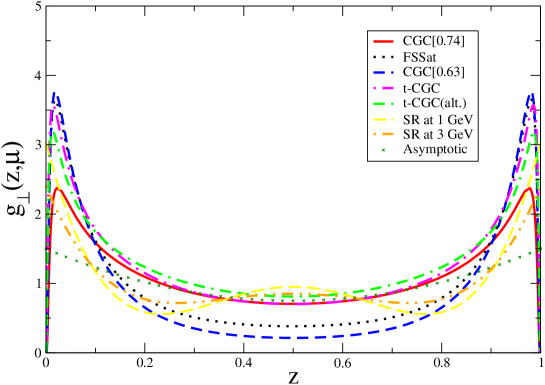
Figure 8: The extracted twist-$3$ DAs compared to the QCD Sum Rules predictions. Dotted: FSSat; Solid: CGC[$0.74$]; Dashed: CGC[$0.63$]; Dot-dashed: t-CGC; Dash-dash-dotted: t-CGC (alt.); Long-dashed: Sum Rules at $1$ GeV; Dot-dot-dashed: Sum Rules at $3$ GeV. Crosses: Asymptotic.

In figure 9, we show our extracted twist-$2$ DAs which are sensitive to the longitudinal wavefunction, i.e. computed using equation (53). Similar predictions appeared in reference [1, 2] for the FSSat and the forward CGC models. We now also show the twist-$2$ DA extracted with the non-forward t-CGC model and in addition we use equation (53) to compute the DA instead of assuming that the DA is simply proportional to the scalar light-cone wavefunction integrated over transverse momentum [47].

The extracted DAs are all consistent with the QCD Sum Rule prediction at $1$ GeV, given the size of the uncertainty on the parameter $a_{2}^{\parallel}$. Table 3 compares the corresponding second moments of the twist-$2$ DA given by

$$\langle\xi^{2}\rangle_{\mu}=\int_{0}^{1}\mathrm{d}z\;\xi^{2}\phi_{\parallel}(z,\mu)\;.$$ (61)

We also show in this table the prediction of the old Boosted Gaussian wavefunction which does not fit the HERA data.

Moments of the leading twist DA at the scale $\mu$

$$\begin{array}[c]{|c|c|c|c|}\hline\cr\mbox{Reference}&\mbox{Approach}&\mbox{Scale}~{}\mu&\langle\xi^{2}\rangle_{\mu}\\ \hline\cr\mbox{\cite[cite]{[\@@bibref{}{Forshaw:2010py}{}{}]}}&\mbox{Old BG prediction}&\sim 1~{}\mbox{GeV}&0.181\\ \hline\cr\mbox{This paper}&\mbox{FSSat fit}&\sim 1~{}\mbox{GeV}&0.267\\ \hline\cr\mbox{This paper}&\mbox{CGC[$0.74$]}&\sim 1~{}\mbox{GeV}&0.266\\ \hline\cr\mbox{This paper}&\mbox{CGC[$0.63$]}&\sim 1~{}\mbox{GeV}&0.271\\ \hline\cr\mbox{This paper}&\mbox{t-CGC}&\sim 1~{}\mbox{GeV}&0.286\\ \hline\cr\mbox{\cite[cite]{[\@@bibref{}{Boyle:2008nj}{}{}]}}&\mbox{Lattice}&2~{}\mbox{GeV}&0.24(4)\\ \hline\cr\mbox{\cite[cite]{[\@@bibref{}{Ball:2007zt}{}{}]}}&\mbox{Sum Rules}&1~{}\mbox{GeV}&0.254\\ \hline\cr\mbox{\cite[cite]{[\@@bibref{}{Ball:2007zt}{}{}]}}&\mbox{Sum Rules}&3~{}\mbox{GeV}&0.237\\ \hline\cr&6z(1-z)&\infty&0.2\\ \hline\cr\end{array}$$

Table 3: Our extracted values for $\langle\xi^{2}\rangle_{\mu}$, compared to predictions based on the QCD Sum Rules or lattice QCD. Note that the Sum Rules prediction at $\mu=1$ GeV has an uncertainty of $\pm 0.024$ corresponding to the uncertainty of $0.07$ in $a_{2}^{\parallel}$.

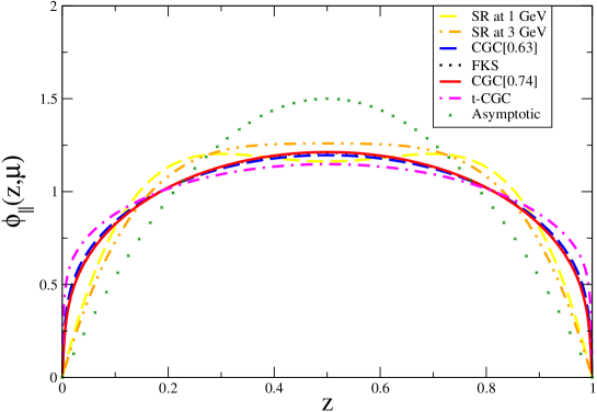
Figure 9: The extracted leading twist-$2$ DAs compared to the Sum Rule predictions. Dotted: FSSat; Solid: CGC[$0.74$]; Dashed: CGC[$0.63$]; Dot-dashed: t-CGC; Long-dashed: Sum Rules at $1$ GeV; Dot-dot-dashed: Sum Rules at $3$ GeV. Crosses: Asymptotic.

8 Conclusions

We have extracted the leading twist-$2$ and subleading twist-$3$ Distribution Amplitudes of the $\rho$ meson using the HERA data. We find that the twist-$2$ DA is not much model dependent where as the data allow for a family of extracted twist-$3$ DAs with a varying degree of end-point enhancement. The extracted DAs are consistent with the QCD Sum Rules and lattice predictions.

In its present form, our parametrization for the DA lacks the perturbative QCD evolution. Improving this would enable a more precise comparison with Sum Rules and the lattice.

9 Acknowledgements

R.S. acknowledges the hospitality of the Particle Physics Group of the University of Manchester where parts of this work were carried out. We thank M. Diehl for useful discussions. This research is supported by the UK’s STFC.

References

• [1] J. R. Forshaw and R. Sandapen, Extracting the rho meson wavefunction from HERA data, JHEP 11 (2010) 037, [arXiv:1007.1990].
• [2] D. Boer et. al., Gluons and the quark sea at high energies: distributions, polarization, tomography, arXiv:1108.1713.
• [3] ZEUS Collaboration, S. Chekanov et. al., Exclusive $\rho^{0}$ production in deep inelastic scattering at HERA, PMC Phys. A1 (2007) 6, [arXiv:0708.1478].
• [4] The H1 Collaboration, Diffractive Electroproduction of $\rho$ and $\phi$ Mesons at HERA, JHEP 05 (2010) 032, [arXiv:0910.5831].
• [5] RBC Collaboration, P. A. Boyle et. al., Parton Distribution Amplitudes and Non-Perturbative Renormalisation, PoS LATTICE2008 (2008) 165, [arXiv:0810.1669].
• [6] P. Ball, V. M. Braun, and A. Lenz, Twist-4 Distribution Amplitudes of the K and $\phi$ Mesons in QCD, JHEP 08 (2007) 090, [arXiv:0707.1201].
• [7] J. R. Forshaw, R. Sandapen, and G. Shaw, Further success of the colour dipole model, JHEP 11 (2006) 025, [hep-ph/0608161].
• [8] C. Marquet, A unified description of diffractive deep inelastic scattering with saturation, Phys. Rev. D76 (2007) 094017, [arXiv:0706.2682].
• [9] G. Watt and H. Kowalski, Impact parameter dependent colour glass condensate dipole model, Phys. Rev. D78 (2008) 014016, [arXiv:0712.2670].
• [10] C. Marquet, R. B. Peschanski, and G. Soyez, Exclusive vector meson production at HERA from QCD with saturation, Phys. Rev. D76 (2007) 034011, [hep-ph/0702171].
• [11] H. Kowalski, L. Motyka, and G. Watt, Exclusive diffractive processes at HERA within the dipole picture, Phys. Rev. D74 (2006) 074016, [hep-ph/0606272].
• [12] J. Bartels, K. J. Golec-Biernat, and H. Kowalski, A modification of the saturation model: DGLAP evolution, Phys. Rev. D66 (2002) 014001, [hep-ph/0203258].
• [13] N. N. Nikolaev and B. G. Zakharov, Colour transparency and scaling properties of nuclear shadowing in deep inelastic scattering, Z. Phys. C49 (1991) 607–618.
• [14] A. H. Mueller and B. Patel, Single and double BFKL pomeron exchange and a dipole picture of high-energy hard processes, Nucl. Phys. B425 (1994) 471–488, [hep-ph/9403256].
• [15] L. Motyka, K. Golec-Biernat, and G. Watt, Dipole models and parton saturation in ep scattering, arXiv:0809.4191.
• [16] C. Ewerz, A. von Manteuffel, and O. Nachtmann, On the Energy Dependence of the Dipole-Proton Cross Section in Deep Inelastic Scattering, arXiv:1101.0288.
• [17] J. R. Forshaw, G. Kerley, and G. Shaw, Extracting the dipole cross-section from photo- and electro-production total cross-section data, Phys. Rev. D60 (1999) 074012, [hep-ph/9903341].
• [18] I. Balitsky, Operator expansion for high-energy scattering, Nucl. Phys. B463 (1996) 99–160, [hep-ph/9509348].
• [19] Y. V. Kovchegov, Small-x F2 structure function of a nucleus including multiple pomeron exchanges, Phys. Rev. D60 (1999) 034008, [hep-ph/9901281].
• [20] Y. V. Kovchegov, Unitarization of the BFKL pomeron on a nucleus, Phys. Rev. D61 (2000) 074018, [hep-ph/9905214].
• [21] J. Jalilian-Marian, A. Kovner, A. Leonidov, and H. Weigert, The BFKL equation from the Wilson renormalization group, Nucl. Phys. B504 (1997) 415–431, [hep-ph/9701284].
• [22] J. Jalilian-Marian, A. Kovner, A. Leonidov, and H. Weigert, The Wilson renormalization group for low x physics: Towards the high density regime, Phys. Rev. D59 (1999) 014014, [hep-ph/9706377].
• [23] E. Iancu, A. Leonidov, and L. D. McLerran, Nonlinear gluon evolution in the color glass condensate. I, Nucl. Phys. A692 (2001) 583–645, [hep-ph/0011241].
• [24] E. Iancu, A. Leonidov, and L. D. McLerran, The renormalization group equation for the color glass condensate, Phys. Lett. B510 (2001) 133–144, [hep-ph/0102009].
• [25] H. Weigert, Unitarity at small Bjorken x, Nucl. Phys. A703 (2002) 823–860, [hep-ph/0004044].
• [26] J. Berger and A. Stasto, Numerical solution of the nonlinear evolution equation at small x with impact parameter and beyond the LL approximation, Phys. Rev. D83 (2011) 034015, [arXiv:1010.0671].
• [27] E. Iancu, K. Itakura, and S. Munier, Saturation and BFKL dynamics in the HERA data at small x, Phys. Lett. B590 (2004) 199–208, [hep-ph/0310338].
• [28] G. Soyez, Saturation QCD predictions with heavy quarks at HERA, Phys. Lett. B655 (2007) 32–38, [arXiv:0705.3672].
• [29] H1 Collaboration, C. Adloff et. al., Elastic electroproduction of $\rho$ mesons at HERA, Eur. Phys. J. C13 (2000) 371–396, [hep-ex/9902019].
• [30] J. R. Forshaw and G. Shaw, Gluon saturation in the colour dipole model?, JHEP 12 (2004) 052, [hep-ph/0411337].
• [31] J. L. Albacete and Y. V. Kovchegov, Solving High Energy Evolution Equation Including Running Coupling Corrections, Phys. Rev. D75 (2007) 125021, [arXiv:0704.0612].
• [32] J. L. Albacete, N. Armesto, J. G. Milhano, and C. A. Salgado, Non-linear QCD meets data: A global analysis of lepton- proton scattering with running coupling BK evolution, Phys. Rev. D80 (2009) 034031, [arXiv:0902.1112].
• [33] C. Flensburg, G. Gustafson, and L. Lonnblad, Elastic and quasi-elastic $pp$ and $\gamma^{*}p$ scattering in the Dipole Model, Eur. Phys. J. C60 (2009) 233–247, [arXiv:0807.0325].
• [34] M. V. T. Machado, Nuclear DVCS at small-x using the color dipole phenomenology, Eur. Phys. J. C59 (2009) 769–776, [arXiv:0810.3665].
• [35] V. P. Goncalves, M. S. Kugeratski, M. V. T. Machado, and F. S. Navarra, Exclusive vector meson production in electron-ion collisions, Phys. Rev. C80 (2009) 025202, [arXiv:0905.1143].
• [36] E. Levin and A. H. Rezaeian, Gluon saturation and inclusive hadron production at LHC, Phys. Rev. D82 (2010) 014022, [arXiv:1005.0631].
• [37] P. Tribedy and R. Venugopalan, Saturation models of HERA DIS data and inclusive hadron distributions in p+p collisions at the LHC, Nucl. Phys. A850 (2011) 136–156, [arXiv:1011.1895].
• [38] J. R. Forshaw, R. Sandapen, and G. Shaw, Colour dipoles and $\rho$, $\phi$ electroproduction, Phys. Rev. D69 (2004) 094013, [hep-ph/0312172].
• [39] G. P. Lepage and S. J. Brodsky, Exclusive Processes in Perturbative Quantum Chromodynamics, Phys. Rev. D22 (1980) 2157.
• [40] J. Nemchik, N. N. Nikolaev, E. Predazzi, and B. G. Zakharov, Color dipole phenomenology of diffractive electroproduction of light vector mesons at HERA, Z. Phys. C75 (1997) 71–87, [hep-ph/9605231].
• [41] P. Ball and V. M. Braun, The $\rho$ Meson Light-Cone Distribution Amplitudes of Leading Twist Revisited, Phys. Rev. D54 (1996) 2182–2193, [hep-ph/9602323].
• [42] P. Ball and V. M. Braun, Handbook of higher twist distribution amplitudes of vector mesons in QCD, hep-ph/9808229.
• [43] I. V. Anikin, D. Y. Ivanov, B. Pire, L. Szymanowski, and S. Wallon, QCD factorization of exclusive processes beyond leading twist: $\gamma^{*T}\rightarrow\rho^{T}$ impact factor with twist three accuracy, Nucl. Phys. B828 (2010) 1–68, [arXiv:0909.4090].
• [44] P. Ball and V. M. Braun, Higher twist distribution amplitudes of vector mesons in QCD: Twist-4 distributions and meson mass corrections, Nucl. Phys. B543 (1999) 201–238, [hep-ph/9810475].
• [45] J. B. Kogut and L. Susskind, Parton models and asymptotic freedom, Phys. Rev. D9 (1974) 3391–3399.
• [46] M. Diehl, Generalized parton distributions in impact parameter space, Eur. Phys. J. C25 (2002) 223–232, [hep-ph/0205208].
• [47] S. J. Brodsky, L. Frankfurt, J. F. Gunion, A. H. Mueller, and M. Strikman, Diffractive leptoproduction of vector mesons in QCD, Phys. Rev. D50 (1994) 3134–3144, [hep-ph/9402283].