The $L$-$\sigma$ Relation of Local Hii Galaxies

Abstract

We present for the first time a new data set of emission line widths for 118 star-forming regions in Hii galaxies (HiiGs). This homogeneous set is used to investigate the $L$-$\sigma$ relation in conjunction with optical spectrophotometric observations. We were able to classify their nebular emission line profiles due to our high resolution spectra. Peculiarities in the line profiles such as sharp lines, wings, asymmetries, and in some cases more than one component in emission were verified. From a new independent homogeneous set of spectrophotometric data we derived physical condition parameters and performed the statistical principal component analysis. We have investigated the potential role of metallicity (O/H), H$\beta$ equivalent width ($W_{\scriptsize\mbox{H}\beta}$) and ionization ratio [OIII]/[OII] to account for the observational scatter of $L$-$\sigma$ relation. Our results indicate that the $L$-$\sigma$ relation for HiiGs is more sensitive to the evolution of the current starburst event (short-term evolution) and dated by $W_{\scriptsize\mbox{H}\beta}$ or even the [OIII]/[OII] ratio. The long-term evolution measured by O/H also plays a potential role in determining the luminosity of the current burst for a given velocity dispersion and age as previously suggested. Additionally, galaxies showing Gaussian line profiles present more tight correlations indicating that they are best targets for the application of the parametric relations as an extragalactic cosmological distance indicator. Best fits for a restricted homogeneous sample of 45 HiiGs provide us a set of new extragalactic distance indicators with an RMS scatter compatible with observational errors of $\delta\log L_{\scriptsize\mbox{H}\alpha}$ = 0.2 dex or 0.5 mag. Improvements may still come from future optimized observational programs to reduce the observational uncertainties on the predicted luminosities of HiiGs in order to achieve the precision required for the application of these relations as tests of cosmological models.

1 Introduction

Giant Hii regions (GHiiRs) and Hii galaxies (HiiGs) have been intensively studied for almost forty years not only because they are natural laboratories to test astrophysical models (Stasińska & Izotov, 2003, and references therein) but also because they present tight scaling relations which can be useful as extragalactic distance estimators (Melnick et al., 2000; Melnick, 2003; Siegel et al., 2005; Plionis et al., 2009).

The correlations between nebular diameter, luminosity ($L$) and velocity dispersion ($\sigma$) of the ionized gas in GHiiRs were found by Melnick (1977, 1978, 1979) and further investigated by Terlevich & Melnick (1981). Several other works from independent groups have confirmed the existence of these relations for GHiiRs in the Local Group’s magellanic irregular galaxies and in some nearby spirals but there is no agreement about the calibration coefficients (slope and zero point), mainly due to different sample selection, observational data quality and linear fit algorithms (Hippelein, 1986; Melnick et al., 1987; Arsenault & Roy, 1988; Fuentes-Masip et al., 2000; Bosch et al., 2002; Rozas et al., 2006). For HiiGs these studies are more scarce. The first $L$-$\sigma$ calibration was obtained by Melnick, Terlevich, & Moles (1988) (hereafter MTM) with an RMS scatter of $\delta\log L_{\scriptsize\mbox{H}\beta}\sim 0.30$, which is a landmark for follow up achievements. In fact, part of this observed scatter has been proposed to be associated with a second parameter, namely oxygen abundance (MTM) or core radius (Telles & Terlevich, 1993).

Despite the fact that the physical origin of the observed supersonic line widths has been a topic of intense debate in the literature, with no consensus (Terlevich & Melnick, 1981; Tenorio-Tagle et al., 1993; Chu & Kennicutt, 1994; Scalo & Chappell, 1999; Melnick et al., 1999; Tenorio-Tagle et al., 2006; Bordalo et al., 2009), the $L$-$\sigma$ relation remains potentially as a powerful alternative empirical extragalactic distance estimator to the classical Tully-Fisher for spirals and $D_{\scriptsize\mbox{n}}$-$\sigma$ relations for ellipticals. This is still more exciting since Tully-Fisher and $D_{\scriptsize\mbox{n}}$-$\sigma$ relations can only be applied up to redshift $\sim$ 1, where the relation is less affected by natural galaxy evolution with the look-back time (Fernández Lorenzo et al., 2011, 2010). On the other hand, light curves of Supernovae Type Ia (SNIa), which are today the most used technique to obtain such cosmological distances encounters lack of target objects at redshifts above $\sim 1.2$ (Riess et al., 2007).

There are, therefore, two possible roles for the $L$-$\sigma$ relation: (1) to obtain distances to nearby galaxies, mainly in the Local Group, where peculiar velocities are significant compared to cosmological recession velocities and distances to nearby galaxy clusters, where HiiGs can be found in their neighborhood; (2) to obtain distances to intermediate and high redshift galaxies (cosmological distances) to probe the dark energy equation of state parameter through Hubble diagram analysis. Several issues, however, should be further investigated for this latter goal with precision required in the era of “concordance cosmology”: (i) the origin of $\sigma$ - the physical mechanism which produces the observed supersonic motions in the ISM (e.g. gravity, turbulence, feedback, stochastic effects of the ISM, etc.); (ii) the validity of the relation to high redshifts - the identification of bona-fide HiiGs at great distances due to the conspicuous emission lines should allow the validity test, once a homogeneous set of kinematic and spectrophotometric data is gathered; (iii) systematic effects - evolutionary and other effects may affect the relation and may be parameterized (e.g. age of the starburst, metallicity, etc.); (iv) observational errors - spectrophotometric calibration, distance, line width, errors may still be suppressed so that the calibration can be competitive with other distance indicators of cosmological interest, and so that the intrinsic scatter in the relation can be assessed; (v) zero-point calibration - further improvement of the zero-point for HiiGs may be achieved by a revision of the distances for GHiiRs in view of modern observations, and at the same time, test the hypothesis that both classes follow the same relation as proposed by MTM.

Several recent works have investigated the kinematics of star-forming galaxies at high redshifts $z\sim 2-3$ (Law et al., 2009; Erb et al., 2004; Pettini et al., 2001). These authors have shown that most of the galaxies found exhibit high local velocity dispersions $\sim 60-100$ km s^-1, suggesting that even for those galaxies with clear velocity gradients, rotation about a preferred kinematic axis may not be the dominant means of physical support. This is also been confirmed in local HiiGs (Moiseev et al., 2010; Bordalo et al., 2009; Martínez-Delgado et al., 2007; Maíz-Apellániz et al., 1999). Despite the fact that most of these distant galaxies have suffered a more violent, and probably continuous star-formation, which led them to become the normal galaxies found in the local Universe, many of their juvenile physical properties are very similar to those found in local HiiGs. These provide us, therefore, empirical support to speculate about the ambitious goal for using the $L$-$\sigma$ relation to determine distances of high redshift galaxies.

In this paper, we present for the first time a large homogeneous data set of emission line width measurements of over 100 local HiiGs ($z$ $<$ 0.1), doubling the sample of MTM with velocity widths obtained from high resolution spectra. These were combined with a complete set of spectrophotometric data obtained mostly from Kehrig, Telles, & Cuisinier (2004) (hereafter KTC) to produce a new calibration for the $L$-$\sigma$ relation. We investigated the potential role of different systematic effects over the $L$-$\sigma$ relation, such as age, metallicity, aperture and non-Gaussianity of the emission line profiles. We argue that the detailed study of these effects is crucial to identify a homogeneous sample for which the relation is valid, and bring light on its physical interpretation.

The paper is organized as follows. Section 2 describes the data, observations and reductions. The results are presented in §3. In §4 we present our data analysis. We present a discussion about our results in §5 and summarize the conclusions in §6. The Hubble Constant adopted throughout this work is $H_{0}$ = 71 km s^-1 Mpc^-1.

2 Data Sample, Observations and Reductions

2.1 The Sample

We have selected most objects from the Spectrophotometric Catalogue of Hii Galaxies (SCHG) (Terlevich et al., 1991, hereafter T91). It contains many galaxies from Curtis Schmidt-Thin Prism Survey of Tololo (Smith et al., 1976, Tol) and University of Michigan Survey (MacAlpine et al., 1977, UM). The SCHG also contains a few galaxies from the Fairall, Markarian and Zwicky lists (Fairall, 1980; Markarian, 1967; Zwicky et al., 1966, F80, MRK, Zw, respectively). We have also selected HiiGs from smaller surveys such as those produced by Kunth et al. (1981) (POX), Maza et al. (1991) (CTS) and Surace & Comte (1998) (SC98). Cambridge UK Schmidt galaxies (Cam) have been selected from Campbell et al. (1986). Note that some of the HiiGs had their names cataloged in more than one of these lists. Additionally, we have selected some classical starburst galaxies — spiral galaxies with Hii nuclear regions or simply nuclear starburst galaxies — from Montreal Blue Galaxy Survey (MBG) (Coziol et al., 1993). However, the objects NGC 6970, IC 5154, ESO 533-G 014 and MCG -01-57-017 were only presented in a private list from Roger Coziol. Nuclear starburst galaxies are also often present in HiiGs lists due to their similar optical spectroscopic properties (for example, UM 477 and MRK 710). Thus our sample consists of 120 starburst regions in galaxies for which we have obtained line widths from optical high spectral resolution spectroscopy.

Figure 1: The redshift distribution of our sample containing 120 objects. The mean of the distribution is 0.0222, whereas the median is 0.0167.

This sample is not complete in a statistical sense. It is heterogeneous in nature comprising four orders of magnitude in H$\alpha$ luminosity range. Figure 1 shows the redshift distribution of our sample. The mean of the distribution is 0.022, and the median is 0.017. The study including all these galaxies is fundamental to investigate the range of the starburst magnitude for which the $L$-$\sigma$ relation is valid. This is, to date, the largest sample of HiiGs ever studied in order to test and calibrate the local $L$-$\sigma$ relation. This has been possible due to the private agreement between the Observatório Nacional-MCT and the European Southern Observatory (ESO) for the dedicated use of the 1.52m and 2.2m telescopes at La Silla, Chile.

2.2 High Spectral Resolution Spectroscopy

HiiGs are mostly compact objects and the young starburst regions in the cores of these systems dominate the main observational properties, i.e. emission line fluxes and their widths (Telles et al., 2001). More recently, Bordalo et al. (2009) have confirmed with a spatially resolved kinematics study of the prototypical HiiG II Zw 40, using 3D integral field spectroscopy, that the line width measured in the nuclear core is the same as the line width measured over the whole extent of the starburst region, indicating that this kinematic core contains information about the overall dynamics of the warm gas.

Figure 2: Optical wavelength calibrated spectrum of CTS 1006 obtained with the FEROS spectrograph. FEROS is an optical echelle spectrograph covering a wide range in wavelength, thus the most intense lines are shown in separated boxes.

We have decided to use the Fiber-fed Extended Range Optical Spectrograph (FEROS) installed initially on the 1.52m and, later, on the ESO 2.2m telescope at La Silla Observatory in Chile, for the first time to observe galaxies, increasing our sample to the present 120 objects. The target fiber was positioned over the brightest region (nuclear core) of the galaxies. FEROS consists of two fibers coupled to the Cassegrain focus of the telescope by micro lenses, providing a spectral resolution of R = 48000 ($\sigma_{\scriptsize\mbox{inst}}$ = 2.50$\pm$0.20 km s^-1, $\sigma$ = FWHM/2.355). Each of the two fibers has a projected 2.7″ entrance aperture and the target and sky are recorded simultaneously.

The echelle FEROS spectrum covers the whole optical region 3560-9200Å. We have observed 103 galaxies with this instrument in five observational runs in the period between November 2000 and April 2007. The FEROS spectra were recorded in a 2048 $\times$ 4096 15$\mu$m pixel CCD. The basic reduction, extraction and dispersion calibration of the spectra were done by a pipeline routine in MIDAS (François, 1999). It processes Bias and Flat Field calibration in a standard way and applies dispersion calibration to the object spectra from information of a thorium-argon-neon lamp spectrum. The final spectrum is calibrated only in wavelength. Line widths for Balmer H$\beta$ (4861 Å), H$\alpha$ (6563 Å) and [OIII] $\lambda\lambda$4959,5007 were measured for most of the galaxies observed. For four galaxies (Tol 0226-390, CTS 1004, Cam 08-28A and CTS 1038) it was not possible to measure H$\alpha$ widths due to regions of bad pixels in the CCD. An example of a wavelength calibrated FEROS spectrum is shown in Figure 2.

Figure 3: Optical calibrated spectrum of UM 499 obtained with the Coudé spectrograph.

Additional line widths were obtained with the 1.60m telescope at Pico dos Dias Observatory (LNA/Brazil) using a Coudé spectrograph and the 600 l/mm diffraction grating, resulting in a spectral resolution at 6500 Å of 0.75 Å and 0.90 Å (instrumental FWHM) when CCD 48 and CCDs 101/106 were used, respectively. These correspond to $\sigma_{\scriptsize\mbox{inst}}=14.7$ and 17.6 km s^-1, respectively. We observed in the region 6400-6900 Å to obtain line width measurements of the H$\alpha$ line emission. The slit used was 1″ for all observations. We obtained data from five observational runs between February 1997 and March 1999.

Coudé data were reduced in a standard procedure for slit spectra in CCD using IRAF. We used the CCDRED package for Bias and Flat Field reduction and the SPECRED package for extraction and calibration procedures. We extracted the spectra from the brightest knot of the galaxies along the slit. An example of a calibrated Coudé spectrum is shown in Figure 3. The ASCII data files of all line profiles analyzed in this work are available at http://www.on.br/astro/etelles/lsigma.

Table 1 lists all observations including FEROS ones and observations with the spectrograph. Columns 1, 2 and 3 give the galaxy name, and their coordinates (J2000). Columns 4, 5, 6 and 7 show the observation log for the Coudé spectrograph and Columns 8, 9 and 10 show the observation log for the FEROS spectrograph, describing the total exposure times, number of exposures, the detector used (only for Coudé) and date of observations, respectively. The last column 11 shows alternative names for the galaxy.

Table 1: Journal of observations.

			Coudé				FEROS
Galaxy	$\alpha$(2000)	$\delta$(2000)	Total Exp.	Number	Detector	Obs.	Total Exp.	Number	Obs.	Other
			Time ($s$)	of Exp.	(CCD)	Date	Time ($s$)	of Exp.	Date	Name
UM 238 (catalog )	00h24m42.3s	+01d44m02s					3600	1	21/07/2001
MBG 00463-0239 (catalog )	00h48m53.2s	-02d22m55s	3600	3	106	13/09/1998				MRK 557
UM 304 (catalog )	01h06m54.0s	+01d56m44s	5400	3	48	28/07/1997	5400	2	23/11/2000
Tol 0104-388 (catalog )	01h07m02.1s	-38d31m52s					5400	1	10/01/2002	CTS 1001
UM 306 (catalog )	01h10m35.0s	+02d06m51s					5400	2	23/11/2000
UM 307 (catalog )	01h11m30.7s	+01d19m16s	1800	1	48	29/07/1997
UM 323 (catalog )	01h26m46.6s	-00d38m46s					5400	2	21/11/2000
Tol 0127-397 (catalog )	01h29m15.8s	-39d30m38s	1200	1	106	17/09/1998	5400	1	20/11/2000
Tol 0140-420 (catalog )	01h43m03.1s	-41d49m41s					5400	2	24/11/2000
UM 137 (catalog )	01h46m23.9s	+04d16m11s					5400	1	21/07/2001
UM 151 (catalog )	01h57m38.8s	+02d25m24s					3600	1	21/07/2001	MRK 1169
UM 382 (catalog )	01h58m09.3s	-00d06m38s					3600	1	22/07/2001
MBG 01578-6806 (catalog )	01h59m06.0s	-67d52m13s	1200	1	106	12/09/1998				NGC 802
UM 391 (catalog )	02h03m30.4s	+02d33m59s	6000	5	106	14/09/1998	5400	2	22/11/2000	MRK 585
			2400	2	106	15/09/1998
UM 395 (catalog )	02h06m56.8s	+01d41m52s					5400	2	24/11/2000
UM 396 (catalog )	02h07m26.5s	+02d56m55s					5400	2	22/11/2000
UM 408 (catalog )	02h11m23.4s	+02d20m30s					5400	2	22/11/2000
UM 417 (catalog )	02h19m30.2s	-00d59m11s					4200	1	22/07/2001
Tol 0226-390 (catalog )	02h28m12.3s	-38d49m20s	2400	2	106	14/09/1998	7200	2	20/11/2000
CTS 1003 (catalog )	02h32m43.7s	-39d34m27s					5400	1	09/01/2002	Tol 0230-397
MBG 02411-1457 (catalog )	02h43m29.2s	-14d45m16s	4800	4	106	12/09/1998				NGC 1076
Tol 0242-387 (catalog )	02h44m37.9s	-38d34m54s					6300	1	23/07/2001
CTS 1004 (catalog )	03h08m43.3s	-40d24m28s					5400	1	09/01/2002	Tol 0306-405
							4800	2	23/11/2000
CTS 1005 (catalog )	03h59m08.9s	-39d06m25s					3600	1	07/01/2002	Cam 0357-3915
Tol 0440-381 (catalog )	04h42m08.1s	-38d01m11s	2400	2	106	17/09/1998	3600	2	20/11/2000
CTS 1006 (catalog )	04h42m09.5s	-45d25m12s					3600	1	10/01/2002
CTS 1007 (catalog )	04h46m49.4s	-30d08m58s					6000	2	22/11/2000
CTS 1008 (catalog )	04h51m39.6s	-31d53m06s					7200	2	21/11/2000
Tol 0505-387 (catalog )	05h07m00.8s	-38d38m58s					4800	2	23/11/2000
Tol 0510-400 (catalog )	05h11m56.3s	-39d59m47s					5400	1	09/01/2002
Tol 0528-383 (catalog )	05h29m57.4s	-38d18m07s					3600	2	20/11/2000
II ZW 40 (catalog )	05h55m42.6s	+03d23m32s	3600	3	101	05/02/1997	4200	1	21/11/2000
							900	1	28/03/2001
Tol 0559-393 (catalog )	06h00m43.9s	-39d19m07s					3600	1	23/11/2000
Tol 0610-387 (catalog )	06h12m14.2s	-38d46m23s					5400	2	24/11/2000
Tol 0614-375 (catalog )	06h16m13.8s	-37d36m37s					3600	1	16/04/2007
Tol 0633-415 (catalog )	06h35m10.2s	-41d33m42s					4800	2	22/11/2000
							3600	1	14/04/2007
Tol 0645-376 (catalog )	06h46m50.1s	-37d43m22s	1800	1	101	04/02/1997	2700	1	20/11/2000
MRK 1201 (catalog )	07h25m45.7s	+29d57m10s					3600	1	31/03/2001
Cam 0840+1201 (catalog )	08h42m20.9s	+11d50m00s					6000	2	24/11/2000
Cam 0840+1044 (catalog )	08h42m36.6s	+10d33m14s					2700	1	29/03/2001
Cam 08-28A (catalog )	08h45m33.5s	+16d05m46s					1800	1	01/04/2001	MRK 702
MRK 710 (catalog )	09h54m49.5s	+09d16m16s	5400	3	101	05/02/1997	1800	1	01/04/2001	NGC 3049
MRK 711 (catalog )	09h55m11.3s	+13d25m46s					5400	1	07/01/2002
Tol 0957-278 (catalog )	09h59m21.2s	-28d08m00s	7200	4	101	06/02/1997	1800	1	28/03/2001	Tol 2
Tol 1004-296NW (catalog )	10h06m33.1s	-29d56m09s	1200	2	101	03/02/1998
Tol 1004-296SE (catalog )	10h06m33.1s	-29d56m09s	600	1	101	03/02/1998
Tol 1008-286 (catalog )	10h10m18.1s	-28d57m48s					3600	1	14/04/2007	Tol 4
CTS 1011 (catalog )	10h19m21.2s	-22d08m35s					2700	1	01/04/2001
CTS 1012 (catalog )	10h21m21.0s	-21d36m27s					3600	1	14/04/2007
CTS 1013 (catalog )	10h25m05.9s	-19d46m57s					2700	1	28/03/2001
Tol 1025-285 (catalog )	10h27m25.5s	-28d47m33s					5400	2	29/03/2001	Tol 6
Haro 24 (catalog )	10h27m55.4s	+19d29m26s					3600	1	13/04/2007	II Zw 47
CTS 1014 (catalog )	10h35m05.4s	-27d20m08s					4500	1	14/04/2007	Tol 1032-2704
CTS 1016 (catalog )	10h37m30.6s	-24d08m41s					3600	1	31/03/2001
CTS 1017 (catalog )	10h37m40.4s	-25d58m00s					5400	1	09/01/2002
CTS 1018 (catalog )	10h38m06.5s	-26d21m56s					3600	1	31/03/2001
CTS 1019 (catalog )	10h41m03.7s	-22d34m24s					1800	1	01/04/2001
CTS 1020 (catalog )	10h47m44.3s	-20d57m49s					2700	1	01/04/2001
CTS 1022 (catalog )	10h48m40.2s	-19d26m57s					3600	1	29/03/2001
$[$F80$]$ 30 (catalog )	10h56m09.1s	+06d10m22s					1800	1	31/03/2001	MRK 1271,Tol 1053+064
MRK 36 (catalog )	11h04m58.3s	+29d08m23s					1800	1	31/03/2001	Haro 4
UM 439 (catalog )	11h36m36.8s	+00d48m58s	3000	3	101	04/02/1998	3600	1	13/04/2007
UM 448 (catalog )	11h42m12.4s	+00d20m03s	4800	4	101	06/02/1997	3600	1	13/04/2007	MRK 1304
Tol 1147-283 (catalog )	11h50m03.2s	-28d40m17s					3600	1	28/03/2001	Tol 17
UM 455 (catalog )	11h50m23.8s	-00d31m41s					2700	1	31/03/2001
UM 456 (catalog )	11h50m36.3s	-00d34m03s					3600	1	13/04/2007
UM 461 (catalog )	11h51m33.3s	-02d22m22s					1800	1	31/03/2001
UM 463 (catalog )	11h52m47.5s	-00d40m08s					3600	1	01/04/2001
CTS 1026 (catalog )	12h05m59.3s	-27d00m56s					3600	1	14/04/2007
UM 477 (catalog )	12h08m11.1s	+02d52m42s	2400	3	101	03/02/1998	3600	1	10/01/2002	MRK 1466,NGC 4123
UM 483 (catalog )	12h12m14.7s	+00d04m20s					5400	1	22/07/2001	MRK 1313
CTS 1027 (catalog )	12h15m18.3s	+05d45m40s					3600	1	16/04/2007	Haro 6
MRK 1318 (catalog )	12h19m09.9s	+03d51m21s	1800	2	106	14/03/1999	3600	1	29/03/2001	Haro 8
CTS 1028 (catalog )	12h23m16.6s	+04d50m09s					3600	1	01/04/2001	Tol 1220+051,[F80] 34
UM 499 (catalog )	12h25m42.8s	+00d34m21s	2400	2	101	04/02/1997
			1200	1	101	05/02/1997
Tol 1223-359 (catalog )	12h25m46.9s	-36d14m01s					3600	1	28/03/2001	Tol 65
Haro 30 (catalog )	12h37m41.1s	+27d07m46s					3600	1	13/04/2007	MRK 650,IC 3600
[SC98] 01 (catalog )	13h04m15.2s	-22d52m53s					3600	1	29/03/2001
CTS 1029 (catalog )	13h06m05.1s	-22d37m22s					6300	2	30/03/2001	[SC98] 09
[SC98] 11 (catalog )	13h06m19.3s	-22d58m49s					4500	1	16/04/2007
UM 559 (catalog )	13h17m42.8s	-01d00m01s					3600	1	28/03/2001
[SC98] 68 (catalog )	13h21m50.0s	-22d28m31s					3600	1	31/03/2001
UM 570 (catalog )	13h23m47.4s	-01d32m52s					4500	1	22/07/2001
[SC98] 88 (catalog )	13h25m33.0s	-26d02m50s					4500	1	29/03/2001
CTS 1030 (catalog )	13h25m33.3s	-25d55m33s					3600	1	14/04/2007	[SC98] 84
POX 186 (catalog )	13h25m48.6s	-11d36m38s					4500	1	01/04/2001
							4500	1	13/04/2007
CTS 1031 (catalog )	13h25m58.5s	-23d38m09s					4500	1	16/04/2007	[SC98] 91
Tol 1345-420 (catalog )	13h48m22.2s	-42d21m15s	600	1	106	14/03/1999	3600	1	30/03/2001	Tol 111
CTS 1033 (catalog )	13h49m44.8s	-18d11m28s					3600	1	13/04/2007
Tol 1400-397 (catalog )	14h03m05.7s	-40d02m28s					7200	1	23/07/2001	Tol 115
UM 649 (catalog )	14h14m27.7s	-00d28m08s					5400	1	21/07/2001
CTS 1034 (catalog )	14h19m32.4s	-27d35m08s					5400	2	28/03/2001
II ZW 70 (catalog )	14h50m56.5s	+35d34m18s					1400	1	28/03/2001	MRK 829
CTS 1035 (catalog )	14h57m19.7s	-22d23m35s					3600	1	30/03/2001
							3600	1	31/03/2001
CTS 1037 (catalog )	15h15m44.0s	-18d18m52s					4300	1	13/04/2007
Cam 1543+0907 (catalog )	15h45m38.6s	+09d03m28s					3600	1	31/03/2001
Tol 1924-416 (catalog )	19h27m58.2s	-41d34m32s	3600	2	48	28/07/1997
Tol 1939-419 (catalog )	19h33m32.0s	-41d50m56s					3100	1	16/04/2007
Tol 1937-423 (catalog )	19h40m58.6s	-42d15m45s	2400	2	106	16/09/1998	5400	1	21/07/2001
CTS 1038 (catalog )	19h54m52.6s	-32d56m40s					4500	1	01/04/2001
CTS 1039 (catalog )	20h05m51.3s	-45d28m42s					3600	1	16/04/2007
Tol 2010-382 (catalog )	20h14m06.4s	-38d07m41s	5400	3	48	29/07/1997	3600	1	14/04/2007
Tol 2019-405 (catalog )	20h23m06.2s	-40d20m33s					5400	1	21/07/2001
Tol 2041-394 (catalog )	20h44m50.8s	-39d13m17s					5400	1	22/07/2001
NGC 6970 (catalog )	20h52m09.4s	-48d46m40s	2400	2	48	28/07/1997
MBG 20533-4410 (catalog )	20h56m43.4s	-43d59m10s	4800	4	48	28/07/1997				NGC 6983
Tol 2122-408 (catalog )	21h25m46.9s	-40d39m12s	4800	4	106	16/09/1998	3600	1	21/11/2000
Tol 2138-405 (catalog )	21h41m21.8s	-40d19m06s					5400	1	23/07/2001
Tol 2138-397 (catalog )	21h41m38.4s	-39d31m30s					1800	1	16/04/2007
Tol 2146-391 (catalog )	21h49m48.2s	-38d54m09s					5400	1	21/07/2001
MBG 21567-1645 (catalog )	21h59m26.1s	-16d30m44s	5400	3	48	29/07/1997				NGC 7165
MBG 22012-1550 (catalog )	22h03m56.3s	-15d36m00s	5400	3	48	29/07/1997
IC 5154 (catalog )	22h04m30.3s	-66d06m45s	2400	2	106	12/09/1998
ESO 533-G 014 (catalog )	22h19m50.6s	-26d20m30s	3600	3	106	12/09/1998
MCG -01-57-017 (catalog )	22h38m13.5s	-07d02m05s	2400	2	106	14/09/1998
Tol 2240-384 (catalog )	22h43m32.4s	-38d11m24s					5400	1	22/07/2001
							3600	1	23/07/2001
MBG 23121-3807 (catalog )	23h14m52.3s	-37d51m20s	8700	8	106	11/09/1998
Tol 2326-405 (catalog )	23h28m49.4s	-40d15m26s					4500	1	23/07/2001
UM 167 (catalog )	23h36m14.1s	+02d09m19s	3600	2	48	29/07/1997				MRK 538, NGC 7714
UM 191 (catalog )	23h56m59.6s	-02d05m02s	5400	3	48	29/07/1997	7200	2	21/11/2000	MRK 542
			2400	2	106	13/09/1998
			4800	4	106	14/09/1998

2.3 Spectrophotometry

Most of the spectrophotometric data used in this work comes from KTC with 91 objects in common with our FEROS plus Coudé sample. Their data were obtained from a Boller & Chivens spectrograph on the 1.52m ESO telescope. The spectra cover 4000Å in the optical range centered at 5700Å. They have a spectral resolution of 5Å and the entrance slit was 2″. KTC observed with a long slit and in some cases they extracted more than one spectrum for a galaxy, representing different bright regions spatially separated. Additional and complementary data were obtained from recent works and the references will be cited below. Emission line fluxes and equivalent widths of permitted and forbidden line fluxes were gathered from these sources to derive the physical parameters, such as extinction coefficient, ionization ratio, electron temperature and density and oxygen abundance.

Table 2: Measurements of redshifts, distances and line widths from FEROS and Coudé spectra. The last column indicates the class of the galaxies discussed in the text.

Galaxy	$z_{\scriptsize\mbox{hel}}$	$D$	FWHM	FWHM	FWHM	FWHM	FWHM	Class
		Mpc	H$\beta$	[OIII] 4959Å	[OIII] 5007Å	H$\alpha$	H$\alpha$ (Coudé)
UM 238	0.01427	55.3	0.844	0.775	0.785	1.158	-	G
MBG 00463-0239	0.01328	51.4	-	-	-	-	3.200	I
UM 304	0.01570	61.7	3.063	3.556	3.444	4.140	4.107	C
Tol 0104-388	0.02263	92.4	1.914	1.880	1.988	2.618	-	I
UM 306	0.01649	65.1	0.846	0.703	0.736	1.147	-	G
UM 307	0.02249	90.4	-	-	-	-	2.772	G
UM 323	0.00648	23.0	0.873	0.853	0.786	1.143	-	G′
Tol 0127-397	0.01735	70.3	1.510	1.420	1.440	1.950	2.045	G′
Tol 0140-420	0.02205	89.9	1.193	1.092	1.104	1.510	-	C
UM 137	0.00591	20.8	-	-	0.676	0.962	-	G
UM 151	0.01607	63.9	1.196	0.892	1.066	1.760	-	G
UM 382	0.01206	47.0	0.812	0.772	0.742	1.028	-	G
MBG 01578-6806	0.00490	19.8	-	-	-	-	1.669	G
UM 391	0.02101	84.9	2.291	-	3.188	3.168	3.320	C
UM 395	0.02234	90.6	1.255	1.281	1.206	1.711	-	G′
UM 396	0.02078	84.0	1.134	1.099	1.110	1.517	-	G′
UM 408	0.01153	45.0	0.867	0.661	0.681	1.165	-	G′
UM 417	0.00872	33.3	0.639	0.544	0.606	0.994	-	G′
Tol 0226-390	0.04771	199.2	3.620	3.410	3.346	-	4.219	I
CTS 1003	0.01684	68.9	1.055	1.005	1.000	1.452	-	G
MBG 02411-1457	0.00686	26.1	-	-	-	-	2.047	G
Tol 0242-387	0.12635	531.5	4.252	4.966	4.949	5.664	-	I
CTS 1004	0.04734	198.3	1.804	1.780	1.831	-	-	I
CTS 1005	0.07441	313.3	2.082	1.963	1.964	2.772	-	I
Tol 0440-381	0.04082	172.2	1.440	1.308	1.310	1.967	2.776	C
CTS 1006	0.02072	87.5	1.492	1.341	1.360	2.032	-	G′
CTS 1007	0.04130	174.2	1.255	1.123	1.108	1.648	-	G′
CTS 1008	0.06106	257.7	2.030	1.891	1.910	2.693	-	G′
Tol 0505-387	0.02897	122.6	0.967	0.812	0.906	1.269	-	G′
Tol 0510-400	0.04132	174.9	1.425	1.282	1.281	1.795	-	G′
Tol 0528-383	0.01163	49.8	0.826	0.760	0.794	1.188	-	G′
II ZW 40	0.00258	11.8	1.329	1.277	1.300	1.826	1.951	I
Tol 0559-393	0.04478	190.3	2.073	1.713	1.929	2.677	-	G
Tol 0610-387	0.00575	25.7	0.771	-	0.929	1.199	-	G
Tol 0614-375	0.03157	134.8	1.820	2.045	2.036	2.646	-	G′
Tol 0633-415	0.01640	71.1	1.310	1.223	1.251	1.705	-	G′
Tol 0645-376	0.02579	110.9	1.229	1.228	1.198	1.708	1.670	G′
MRK 1201	0.01857	80.6	1.843	-	-	2.491	-	G
Cam 0840+1201	0.02938	128.2	1.510	1.397	1.400	1.945	-	G′
Cam 0840+1044	0.01044	48.0	0.752	0.549	0.573	0.999	-	G′
Cam 08-28A	0.05304	227.8	2.090	1.797	1.856	-	-	I
MRK 710	0.00502	25.9	2.201	-	2.127	2.708	2.697	C
MRK 711	0.01944	86.7	3.685	3.418	3.499	5.046	-	I
Tol 0957-278	0.00334	18.8	1.031	1.051	1.044	1.503	1.543	I
Tol 1004-296NW	0.00370	20.2	-	-	-	-	1.943	I
Tol 1004-296SE	0.00359	19.8	-	-	-	-	1.738	G
Tol 1008-286	0.01384	63.1	1.054	1.010	1.008	1.455	-	G′
CTS 1011	0.01207	55.9	0.921	0.823	0.837	1.241	-	G′
CTS 1012	0.01089	50.9	0.787	0.650	0.646	1.051	-	G′
CTS 1013	0.02688	118.5	1.390	1.346	1.380	1.774	-	C
Tol 1025-285	0.03073	134.5	2.356	-	2.438	2.986	-	G
Haro 24	0.04327	187.3	1.770	1.587	1.759	2.565	-	I
CTS 1014	0.05895	253.8	2.333	1.778	1.849	2.803	-	I
CTS 1016	0.03450	150.6	1.456	1.323	1.410	2.203	-	I
CTS 1017	0.03544	154.5	1.186	1.176	1.176	1.598	-	G′
CTS 1018	0.03925	170.6	1.453	1.313	1.316	1.977	-	G
CTS 1019	0.06651	285.8	1.888	1.895	1.936	2.761	-	G′
CTS 1020	0.01248	57.7	1.393	1.365	1.399	1.911	-	G′
CTS 1022	0.01369	62.9	0.974	0.839	0.854	1.427	-	G
$[$F80$]$ 30	0.00335	18.2	0.903	0.741	0.749	1.205	-	G′
MRK 36	0.00212	13.2	0.782	0.687	0.717	1.051	-	G′
UM 439	0.00382	21.3	0.805	0.708	0.711	1.103	1.444	G′
UM 448	0.01834	82.6	2.947	3.043	3.017	4.143	3.376	C
Tol 1147-283	0.00626	31.2	0.793	0.799	0.724	1.113	-	G′
UM 455	0.01306	60.3	0.998	0.746	0.740	1.518	-	I
UM 456	0.00572	29.3	0.757	0.631	0.643	1.017	-	G′
UM 461	0.00352	20.0	0.669	0.512	0.519	0.912	-	G′
UM 463	0.00468	24.9	0.849	0.680	0.676	1.057	-	G′
CTS 1026	0.00577	29.2	1.710	1.689	1.705	2.284	-	G
UM 477	0.00422	22.8	2.243	-	2.860	3.019	3.038	C
UM 483	0.00792	38.4	0.816	0.776	0.744	1.105	-	I
CTS 1027	0.00674	33.4	0.892	0.799	0.821	1.217	-	I
MRK 1318	0.00504	26.2	0.756	0.680	0.695	1.052	1.448	G′
CTS 1028	0.01776	79.9	1.141	1.074	1.098	1.520	-	C
UM 499	0.00707	34.8	-	-	-	-	2.520	I
Tol 1223-359	0.00930	44.2	0.828	0.681	0.707	1.163	-	G′
Haro 30	0.01552	69.5	1.746	1.887	1.845	2.428	-	I
$[$SC98$]$ 01	0.01041	48.4	0.975	0.791	0.720	1.185	-	G′
CTS 1029	0.03633	157.8	-	-	-	1.787	-	G
$[$SC98$]$ 11	0.03104	135.5	1.317	1.285	1.244	1.801	-	I
UM 559	0.00429	22.5	0.794	0.676	0.687	1.103	-	G′
$[$SC98$]$ 68	0.02377	104.7	1.274	1.346	1.300	1.758	-	G
UM 570	0.02249	99.3	0.930	0.884	0.867	1.291	-	G′
$[$SC98$]$ 88	0.01454	65.6	1.066	0.896	0.860	1.491	-	I
CTS 1030	0.01505	67.7	1.221	1.213	1.212	1.668	-	C
POX 186	0.00415	21.9	0.715	0.584	0.586	0.984	-	G′
CTS 1031	0.04525	195.3	1.338	1.296	1.386	1.770	-	I
Tol 1345-420	0.00807	37.5	0.877	0.743	0.791	1.188	1.655	G′
CTS 1033	0.01549	69.4	1.921	1.935	1.939	2.602	-	C
Tol 1400-397	0.03101	134.3	1.352	1.299	1.368	1.922	-	G′
UM 649	0.02611	113.9	1.152	0.935	1.018	1.480	-	G
CTS 1034	0.02292	100.2	-	1.091	1.037	1.533	-	G
II ZW 70	0.00406	19.2	0.901	0.794	0.823	1.377	-	G′
CTS 1035	0.02848	123.2	1.164	1.120	1.086	1.409	-	G
CTS 1037	0.02130	92.5	1.562	1.530	1.513	2.074	-	I
Cam 1543+0907	0.03766	160.8	1.293	1.186	1.179	1.716	-	G′
Tol 1924-416	0.00952	38.4	-	-	-	-	2.065	I
Tol 1939-419	0.02525	104.8	-	-	0.962	1.336	-	G
Tol 1937-423	0.00932	37.4	1.022	0.768	0.888	1.262	1.874	G
CTS 1038	0.04984	208.0	-	2.123	2.136	-	-	I
CTS 1039	0.04486	187.4	1.693	1.704	1.722	2.287	-	I
Tol 2010-382	0.02026	83.0	1.506	-	1.480	1.899	2.166	G′
Tol 2019-405	0.01495	60.6	1.095	0.978	0.996	1.300	-	I
Tol 2041-394	0.02576	106.0	-	1.178	1.121	1.627	-	G
NGC 6970	0.01751	71.6	-	-	-	-	2.594	C
MBG 20533-4410	0.01714	69.7	-	-	-	-	3.075	C
Tol 2122-408	0.01480	59.4	1.114	1.052	1.071	1.416	1.717	G
Tol 2138-405	0.05802	241.7	2.445	2.468	2.496	3.444	-	C
Tol 2138-397	0.01570	63.0	0.996	0.998	0.900	1.391	-	G′
Tol 2146-391	0.02953	121.3	1.154	0.935	0.991	1.503	-	I
MBG 21567-1645	0.01738	68.8	-	-	-	-	5.513	C
MBG 22012-1550	0.04227	173.9	-	-	-	-	5.074	C
IC 5154	0.01068	43.7	-	-	-	-	2.035	G
ESO 533-G 014	0.00873	32.6	-	-	-	-	1.317	G
MCG -01-57-017	0.00962	35.6	-	-	-	-	1.567	G
Tol 2240-384	0.07584	316.6	2.082	2.112	2.196	2.940	-	C
MBG 23121-3807	0.00945	36.2	-	-	-	-	1.777	G
Tol 2326-405	0.05515	229.3	-	-	1.556	2.456	-	I
UM 167	0.00928	34.0	-	-	-	-	3.925	G
UM 191	0.02427	97.4	1.265	-	1.584	1.798	2.000	G′

3 Results

3.1 Line Widths and Velocity Dispersions

We have measured the emission line widths from our high spectral resolution observations by fitting single Gaussians to the observed line profiles using the SPLOT routine of IRAF. The H$\alpha$ line for the Coudé spectra were measured and H$\alpha$, H$\beta$ and [OIII] $\lambda\lambda$4959,5007 lines for FEROS spectra were detected and measured for almost all galaxies. All observed FWHM, uncorrected for instrumental width, are presented in Table 2.

In several cases a single Gaussian fit did not adequately represent the observed profile. Some present irregularities such as prominent wings and multiple components. Different methodologies to obtain line widths such as multiple Gaussians or Gauss-Hermite (Riffel, 2010, and references therein) fits are viable approaches to the problem of modeling real emission line profiles, and were tested. For instance, Gauss-Hermite fits provide single width measurements that are well compared with single Gaussian fit measurements, and they are less sensitive to small asymmetries. In the case of profiles with a dominant broad component or with double peaks, multiple Gaussians or Gauss-Hermite methodologies provide better fits. However, the interpretation of the model parameters is not obvious. Further detailed analysis with more data is needed to resolve this issue, but it is beyond the scope of this paper. Here, we are interested in the simplest methodology to measure the line widths that may provide us with a robust kinematic measurement of the starburst region as a whole.

As a simple alternative to deal with this problem, we classified galaxies depending on their line profiles using the following criterion:

• Gaussian Profile - Symmetrical lines well represented by a single Gaussian fit. These profiles occur in 62% of galaxies in our sample.

• Irregular Profile - Asymmetrical lines showing prominent wings and generally peaked. These occur in 29% of our sample.

• Profile with Components - These clearly show more than one component in emission, normally double-peak lines with similar intensities, occurring in 17% of our sample.

Our classification was done by eye comparison between the single Gaussian fit and the observed line profile, therefore it has an intrinsic subjectiveness even though interesting for early and qualitative purposes in this work. Since we have for most galaxies the four strong emission lines, we checked them all to classify the galaxy. Figure 4 presents some examples of prototypical H$\alpha$ profiles of the three classes defined. All galaxies were classified including those showing low signal-to-noise (S/N) in their emission line profiles. Some galaxies may have been classified as presenting Gaussian profiles simply because the line wings were not well sampled. The spectra from FEROS were used in priority to Coudé ones to classify those galaxies observed with both instruments. The galaxies were assigned as letter G for Gaussian and I for irregular profiles, and C for profiles with components. The respective class for each galaxy is shown in the last column of Table 2. We will return to this point later in Section 4.2 using a semi-quantitative analysis of line profile classifications to select a more homogeneous sample.

Figure 4: Examples of the three classes of line profiles visually identified. (first row) Galaxies with nearly Gaussian profiles; (second row) galaxies with irregular profiles; (third row) galaxies with line profiles clearly showing components. The dotted narrow lines in all of the left-hand boxes represent the FEROS instrumental profile, $\sigma_{\scriptsize\mbox{inst}}=2.50$ km s^-1. The dashed lines represent single Gaussian fits to the observed profiles.

Figure 5: (left) Testing the consistency of measurements between $\sigma$ derived from H$\alpha$ and H$\beta$ (FEROS); (center) $\sigma_{\scriptsize\mbox{[OIII]5007\AA}}$ and $\sigma_{\scriptsize\mbox{[OIII]4959\AA}}$; (right) H$\alpha$ from FEROS ($x$) and Coudé ($y$). Tol 0440-381 and UM 448 noted in the right plot present the most discrepant measurements possibly due to different position covered by observations.

We derived the radial velocity dispersions ($\sigma$) from the observed FWHM presented in Table 2. The observed velocity dispersions ($\sigma_{\scriptsize\mbox{obs}}$) in km s^-1 were corrected by the instrumental ($\sigma_{\scriptsize\mbox{inst}}$), and thermal broadening ($\sigma_{\scriptsize\mbox{th}}$), assuming a Maxwellian velocity distribution of the hydrogen and oxygen atoms,

$$\sigma_{\scriptsize\mbox{th}}=\sqrt{\frac{kT_{e}}{m}},$$

where $k$ is the Boltzmann constant, $T_{e}$ is the electronic temperature in Kelvin and $m$ is the mass of the atom. We used $T_{e}(\mbox{OIII})$ presented in Table 3 to derive $\sigma_{\scriptsize\mbox{th}}$ for all galaxies. For those galaxies where $T_{e}$ was not directly determined or found in literature we assumed a mean value of 14000 K. For H lines from FEROS spectra we also corrected $\sigma_{\scriptsize\mbox{obs}}$ by the fine structure broadening ($\sigma_{\scriptsize\mbox{fs}}$): 3.20 km s^-1 for H$\alpha$ and 2.40 km s^-1 for H$\beta$ as adopted by García-Díaz et al. (2008). The velocity dispersion of interest here and sometimes called “non-thermal” velocity dispersion, was calculated by

$$\sigma=\sqrt{\sigma_{\scriptsize\mbox{obs}}^{2}-\sigma_{\scriptsize\mbox{inst}}^{2}-\sigma_{\scriptsize\mbox{th}}^{2}-\sigma_{\scriptsize\mbox{fs}}^{2}}.$$

For the FEROS, $\sigma_{\scriptsize\mbox{inst}}$ = 2.5 km s^-1, while for Coudé, $\sigma_{\scriptsize\mbox{inst}}$ = 14.7 km s^-1 and = 17.6 km s^-1, depending on the instrumentation used (see Section 2.2). The correction due to $\sigma_{\scriptsize\mbox{th}}$ for H lines varies between 9.5 and 12.5 km s^-1, and for the O lines, between 2 and 3 km s^-1. We estimated the error in $\sigma$ due to uncertainties in $T_{e}$ as being $\delta\sigma_{\scriptsize\mbox{H}}<0.3$ km s^-1 and $\delta\sigma_{\scriptsize\mbox{O}}<0.1$ km s^-1.

Table 3: H$\alpha$ integrated fluxes, H$\beta$ extinction coefficients, H$\beta$ equivalent widths, ionization ratios [OIII]/[OII], O/H ratios and electron densities and temperatures.

Galaxy	$F_{\scriptsize\mbox{H}\alpha}$	$C_{\scriptsize\mbox{H}\beta}$	$W_{\scriptsize\mbox{H}\beta}$	[OIII]/[OII]	$N_{e}$	$T_{e}$	12+	Ref.
	(erg s-1 cm-2)		Å		cm-3	$10^{4}$K	$\log(\mbox{O}/\mbox{H})$
UM 238	2.0e-14	0.23	36	3.31	867	1.53	7.89	1,1,1,1,1,1,18
MBG 00463-0239	8.2e-14	0.38	10	0.19	374	1.40	8.70	1,1,1,1,1,22,16
UM 304	1.5e-13	1.09	-	-	204	1.40	-	14,2,-,-,22,22,-
Tol 0104-388	4.7e-14	0.19	60	1.14	846	1.49	7.96	1,1,1,1,1,1,18
UM 306	3.1e-14	0.08	24	2.21	27	1.16	8.18	1,1,1,1,1,1,18
UM 307	1.1e-13	0.25	23	0.67	983	1.40	8.43	1,1,1,1,1,22,16
UM 323	2.6e-14	0.85	21	0.90	27	1.76	7.92	1,1,1,1,1,1,18
Tol 0127-397	4.1e-14	0.51	-	-	204	1.40	-	14,2,-,-,22,22,-
Tol 0140-420	2.3e-14	0.00	56	1.98	27	1.28	8.06	1,1,1,1,1,1,18
UM 137	1.5e-14	0.37	4	0.55	27	1.40	8.25	1,1,1,1,1,22,17
UM 151	2.6e-14	0.41	20	0.79	94	1.40	8.47	1,1,1,15,1,22,17
UM 382	1.9e-14	0.18	135	10.90	45	1.62	7.82	6,6,6,6,6,6,6
MBG 01578-6806	-	-	-	-	204	1.40	-	-,-,-,-,22,22,-
UM 391	5.1e-14	0.54	14	0.35	27	1.40	8.40	1,1,1,1,1,22,16
UM 395	1.6e-14	0.49	6	0.42	579	1.40	8.63	1,1,1,1,1,22,17
UM 396	3.7e-14	0.00	153	5.85	27	1.22	8.18	1,1,1,1,1,1,18
UM 408	2.0e-14	0.06	33	3.66	207	1.33	8.02	1,1,1,1,1,1,18
UM 417	5.8e-15	0.45	46	7.65	27	1.40	8.04	1,1,1,1,1,22,17
Tol 0226-390	1.0e-13	0.31	115	3.03	193	1.16	8.15	1,1,1,1,1,1,18
CTS 1003	2.2e-14	0.24	-	-	204	1.40	7.90	3,3,-,-,22,22,3
MBG 02411-1457	4.7e-14	0.76	2	0.15	132	1.40	8.26	1,1,1,1,1,22,16
Tol 0242-387	1.1e-13	0.78	-	-	204	1.40	8.23	2,2,-,-,22,22,19
CTS 1004	3.5e-14	0.00	77	3.83	101	1.21	8.14	1,1,1,1,1,1,18
CTS 1005	4.3e-14	0.16	134	11.14	204	1.46	7.91	1,1,1,1,22,1,18
Tol 0440-381	5.5e-14	0.11	29	1.77	27	1.53	7.96	1,1,1,1,1,1,18
CTS 1006	1.4e-13	0.15	70	2.88	27	1.28	8.04	1,1,1,1,1,1,18
CTS 1007	4.3e-14	0.01	-	-	204	1.40	7.83	3,3,-,-,22,22,3
CTS 1008	5.7e-14	0.24	140	6.04	278	1.21	8.16	1,1,1,1,1,1,18
Tol 0505-387	1.1e-14	0.35	10	0.66	27	1.40	8.50	1,1,1,1,1,22,17
Tol 0510-400	3.3e-14	0.19	64	2.39	227	1.40	8.25	1,1,1,1,1,22,16
Tol 0528-383	3.7e-14	0.35	21	1.86	133	1.48	7.96	1,1,1,1,1,1,18
II ZW 40	3.5e-13	0.61	184	10.98	217	1.31	8.07	1,1,1,1,1,1,18
Tol 0559-393	4.5e-14	0.35	-	-	204	1.40	-	2,2,-,-,22,22,-
Tol 0610-387	1.1e-14	0.93	4	0.44	27	1.40	8.56	1,1,1,2,1,22,17
Tol 0614-375	6.9e-14	1.25	-	-	204	1.40	7.86	2,2,-,-,22,22,20
Tol 0633-415	1.1e-13	0.40	83	4.59	67	1.25	8.14	1,1,1,21,1,21,4
Tol 0645-376	2.9e-14	0.19	28	1.58	27	1.78	7.77	1,1,1,1,1,1,18
MRK 1201	3.9e-14	0.52	8	0.50	1467	1.40	9.36	1,1,1,1,1,22,16
Cam 0840+1201	1.1e-13	0.03	105	3.53	27	1.32	7.98	1,1,1,1,1,1,18
Cam 0840+1044	2.1e-14	0.25	44	7.85	27	1.58	7.73	1,1,1,1,1,1,18
Cam 08-28A	1.5e-13	0.28	37	1.60	97	1.11	8.13	1,1,1,1,1,1,18
MRK 710	4.5e-13	0.50	29	0.23	184	1.40	8.95	1,1,1,1,1,22,16
MRK 711	1.9e-13	0.54	28	1.61	460	1.40	8.79	1,1,1,2,1,22,17
Tol 0957-278	2.0e-13	0.17	36	1.92	74	1.24	8.02	1,1,1,1,1,1,18
Tol 1004-296NW	7.4e-13	0.40	62	3.50	122	1.04	8.28	1,1,1,1,1,1,18
Tol 1004-296SE	5.0e-13	0.30	52	2.69	69	1.08	8.20	1,1,1,1,1,1,18
Tol 1008-286	5.1e-14	1.05	123	9.55	395	1.30	8.17	1,1,1,21,1,21,4
CTS 1011	6.2e-14	0.34	93	3.80	233	1.28	8.18	1,1,1,1,1,1,18
CTS 1012	6.3e-14	0.01	-	-	204	1.40	8.41	3,3,-,-,22,22,3
CTS 1013	1.7e-14	0.00	38	3.40	185	1.29	8.08	1,1,1,1,1,1,18
Tol 1025-285	4.0e-14	0.79	9	0.31	27	1.40	8.71	1,1,1,2,1,22,17
Haro 24	4.8e-14	0.57	11	0.88	27	1.40	8.23	1,1,1,1,1,22,17
CTS 1014	2.2e-14	0.01	-	-	204	1.40	7.98	3,3,-,-,22,22,3
CTS 1016	1.7e-14	0.19	26	1.24	27	1.40	8.36	1,1,1,1,1,22,3
CTS 1017	2.2e-14	0.22	161	6.68	247	1.46	7.98	1,1,1,1,1,1,18
CTS 1018	1.8e-14	0.16	58	2.43	140	1.40	7.97	1,1,1,1,1,1,18
CTS 1019	4.2e-14	0.22	90	3.87	27	1.11	8.22	1,1,1,1,1,1,18
CTS 1020	1.5e-13	0.33	109	2.94	101	1.12	8.25	1,1,1,1,1,1,18
CTS 1022	2.6e-14	0.43	57	1.53	147	1.33	8.09	1,1,1,1,1,1,18
$[$F80$]$ 30	2.9e-13	0.00	97	5.07	215	1.41	7.99	1,1,1,7,1,7,7
MRK 36	1.5e-13	0.08	62	3.48	96	1.38	7.89	1,1,1,1,1,1,18
UM 439	1.2e-13	0.05	49	4.30	27	1.39	8.01	1,1,1,1,1,1,18
UM 448	7.3e-13	0.40	48	1.16	151	1.08	8.17	1,1,1,1,1,1,18
Tol 1147-283	5.6e-14	0.20	40	1.08	79	1.51	7.88	1,1,1,1,1,1,18
UM 455	2.0e-14	0.48	29	4.32	27	1.73	7.74	1,1,1,1,1,1,18
UM 456	8.9e-14	0.06	44	3.09	27	1.41	7.95	1,1,1,1,1,1,18
UM 461	1.1e-13	0.05	155	9.43	115	1.66	7.77	1,1,1,1,1,1,18
UM 463	3.3e-14	0.17	74	6.08	102	1.32	7.92	1,1,1,20,1,11,11
CTS 1026	1.0e-12	0.33	-	-	204	1.40	8.30	3,3,-,-,22,22,3
UM 477	2.6e-13	0.88	17	0.34	979	1.40	9.12	1,1,1,1,1,22,16
UM 483	4.7e-14	0.45	19	0.84	133	1.71	7.85	1,1,1,11,1,11,11
CTS 1027	1.5e-13	0.08	50	1.88	63	1.01	8.35	8,8,8,8,8,8,8
MRK 1318	2.2e-13	0.27	68	1.70	78	1.01	8.27	1,1,1,1,1,1,18
CTS 1028	4.5e-14	0.57	82	3.90	344	1.40	8.05	1,1,1,1,1,1,18
UM 499	6.1e-13	0.55	24	0.45	611	1.40	8.82	1,1,1,1,1,22,16
Tol 1223-359	7.5e-14	0.16	129	7.18	27	1.73	7.54	1,1,1,12,1,12,12
Haro 30	6.1e-14	0.00	28	0.93	103	1.54	7.67	1,1,1,1,1,1,18
$[$SC98$]$ 01	1.8e-14	0.14	34	1.39	45	1.40	8.27	1,1,1,1,1,22,17
CTS 1029	1.9e-14	0.29	35	1.05	489	1.40	8.42	1,1,1,1,1,22,3
$[$SC98$]$ 11	-	-	-	-	204	1.40	-	-,-,-,-,22,22,-
UM 559	5.0e-14	0.00	535	4.92	204	1.58	7.72	1,1,1,1,22,9,9
$[$SC98$]$ 68	2.1e-14	0.52	22	0.76	343	1.40	8.49	1,1,1,1,1,22,17
UM 570	3.1e-14	0.00	180	43.00	204	1.83	7.71	1,1,1,9,22,9,9
$[$SC98$]$ 88	1.9e-14	0.29	20	1.24	339	1.41	8.02	1,1,1,1,1,1,18
CTS 1030	7.0e-14	0.01	-	-	204	1.40	8.25	3,3,-,-,22,22,3
POX 186	7.2e-14	0.01	274	19.26	342	1.66	7.74	1,1,1,1,1,1,18
CTS 1031	3.4e-14	0.22	-	-	204	1.40	8.23	3,3,-,-,22,22,3
Tol 1345-420	8.7e-14	0.27	51	2.89	71	1.07	8.26	1,1,1,1,1,1,18
CTS 1033	7.4e-14	0.24	59	8.69	155	1.42	8.01	1,1,1,1,1,1,18
Tol 1400-397	2.3e-14	0.20	-	-	204	1.40	-	2,2,-,-,22,22,-
UM 649	1.2e-14	0.00	-	-	204	1.40	-	2,2,-,-,22,22,-
CTS 1034	1.3e-14	0.28	20	1.53	1288	1.47	7.96	1,1,1,1,1,1,18
II ZW 70	2.7e-13	0.30	49	1.90	96	1.21	8.07	5,13,10,10,13,13,4
CTS 1035	1.5e-14	0.12	62	2.91	510	1.40	8.01	1,1,1,1,1,22,3
CTS 1037	4.0e-13	0.29	-	-	204	1.40	8.21	3,3,-,-,22,22,3
Cam 1543+0907	5.9e-14	0.05	192	8.96	74	1.68	7.71	1,1,1,1,1,1,18
Tol 1924-416	1.0e-12	0.11	100	4.86	131	1.35	8.01	1,1,1,1,1,1,18
Tol 1939-419	1.3e-14	0.00	-	-	204	1.40	-	2,2,-,-,22,22,-
Tol 1937-423	2.0e-14	0.70	5	0.49	39	1.40	8.48	1,1,1,1,1,22,17
CTS 1038	1.9e-13	0.53	-	-	204	1.40	7.82	3,3,-,-,22,22,3
CTS 1039	9.7e-14	0.01	-	-	204	1.40	7.70	3,3,-,-,22,22,3
Tol 2010-382	8.2e-14	0.76	-	-	204	1.40	-	14,2,-,-,22,22,-
Tol 2019-405	1.5e-14	0.10	11	1.90	76	1.45	7.99	1,1,1,1,1,1,18
Tol 2041-394	1.9e-14	0.00	-	-	204	1.40	-	2,2,-,-,22,22,-
NGC 6970	9.7e-14	0;00	-	-	204	1.40	-	14,2,-,-,22,22,-
MBG 20533-4410	1.0e-13	0.81	8	0.20	90	1.40	8.88	1,1,1,1,1,22,16
Tol 2122-408	2.6e-14	0.41	14	4.47	97	1.40	8.49	1,1,1,1,1,22,16
Tol 2138-405	8.9e-14	0.19	208	7.08	204	1.38	7.98	9,9,9,9,22,9,9
Tol 2138-397	1.8e-14	0.12	33	2.49	27	1.86	7.64	1,1,1,1,1,1,18
Tol 2146-391	2.8e-14	0.09	246	7.70	47	1.59	7.78	1,1,1,1,1,1,18
MBG 21567-1645	3.2e-14	1.36	2	0.08	281	1.40	8.93	1,1,1,1,1,22,17
MBG 22012-1550	3.9e-14	0.84	7	0.70	27	1.40	8.20	1,1,1,1,1,22,16
IC 5154	4.9e-14	0.38	10	0.79	250	1.40	8.52	1,1,1,1,1,22,17
ESO 533-G 014	5.7e-14	0.45	6	0.41	27	1.51	7.90	1,1,1,1,1,1,18
MCG -01-57-017	6.5e-14	0.10	11	0.23	27	1.40	8.37	1,1,1,1,1,22,16
Tol 2240-384	3.4e-14	0.37	165	8.72	204	1.53	7.85	1,1,1,1,22,1,18
MBG 23121-3807	2.4e-14	0.71	4	0.11	27	1.40	8.75	1,1,1,1,1,22,17
Tol 2326-405	4.1e-14	0.22	-	-	204	1.40	8.03	2,2,-,-,22,22,19
UM 167	1.2e-12	0.26	-	-	204	1.40	-	14,2,-,-,22,22,-
UM 191	3.6e-14	0.43	7	0.26	108	1.40	8.30	1,1,1,1,1,22,16

The internal errors were determined as a function of the S/N calculated for the emission lines and defined as the ratio between the peak intensity and the adjacent continuum RMS. Figure 5 shows the comparisons between $\sigma$ derived from the same ion considering all data. The FEROS measurements are very consistent. The RMS of a linear fit for all points are 1.96 for Hii and 1.36 for [OIII] lines in km s^-1 (Figure 5 left and center). The comparison between FEROS and Coudé measurements also shows good agreement except for two objects (Tol 0440-381 and UM 448) that present components in their line profiles. The observation of these objects is more sensitive to the position of the slit and fiber over the galaxy. The RMS = 5.22 km s^-1 from a linear fit is also shown inside the box (Figure 5 right). For different ranges of S/N we selected samples of galaxies for their $\sigma$ values to be compared. The selection was based on the S/N of the weaker lines of each ion (i.e. H$\beta$ and [OIII]$\lambda$4959) and their $\sigma$ values were plotted in $y$ axis against the $\sigma$ values derived from the more intense line in $x$. The errors were estimated by taking the RMS of a direct least square fit for each data set. In a similar procedure, we estimated the errors for Coudé $\sigma_{\scriptsize\mbox{H}\alpha}$ comparing sets of two ranges of S/N with $\sigma_{\scriptsize\mbox{H}\alpha}$ of galaxies observed also with FEROS. Table 4 shows the estimated errors in $\sigma$ as a function of S/N for H and O lines. The $\sigma$ values and their respective errors for each line are shown in Table 5.

Table 4: Errors in $\sigma$ as a function of signal-to-noise ratio of the line-emission.

S/N	$\delta\sigma_{\scriptsize\mbox{H}}$	S/N	$\delta\sigma_{\scriptsize\mbox{O}}$
H lines	km s-1	O lines	km s-1
FEROS
S/N $<$ 10	2.9	S/N $<$ 10	2.1
10 $<$ S/N $<$ 20	2.2	10 $<$ S/N $<$ 20	1.4
20 $<$ S/N $<$ 30	1.8	20 $<$ S/N $<$ 30	0.9
30 $<$ S/N $<$ 40	1.2	30 $<$ S/N $<$ 50	0.7
40 $<$ S/N $<$ 75	0.7	50 $<$ S/N $<$ 150	0.5
S/N $>$ 75	0.4	S/N $>$ 150	0.2
Coudé
S/N $<$ 110	4.6
S/N $>$ 110	3.5

3.2 Physical Conditions

Before we use line fluxes to derive physical conditions we need to infer the amount of extinction for each galaxy. Dust in starburst regions is responsible for extinction of light in the line of sight due to absorption and scattering. In optical wavelengths, the amount of extinction can be reasonably well estimated from H recombination lines through the Balmer Decrement method. To derive H$\beta$ extinction coefficient ($C_{\scriptsize\mbox{H}\beta}$) for galaxies with KTC spectrophotometry we used the theoretical ratios H$\alpha$/H$\beta$ = 2.87 and H$\gamma$/H$\beta$ = 0.466 for case B optically thick with T = 10⁴ K (Osterbrock 1989). In cases where H$\alpha$/H$\beta$ was smaller than the theoretical value 2.87, we calculated $C_{\scriptsize\mbox{H}\beta}$ using the ratio H$\gamma$/H$\beta$. When ratios were H$\alpha$/H$\beta$ $<$ 2.87 and H$\gamma$/H$\beta$ $>$ 0.466 simultaneously we adopted the zero value for $C_{\scriptsize\mbox{H}\beta}$. Dereddened fluxes $I_{\lambda}$ were thus calculated by

$$I_{\lambda}=F_{\lambda}\exp[C_{\scriptsize\mbox{H}\beta}(1+f_{\lambda})],$$

where $F_{\lambda}$ is the published flux corrected by atmospheric extinction and $f_{\lambda}$ is the interstellar reddening function normalized at H$\beta$. We adopted $f_{\lambda}$ from Whitford (1958) as normalized by Lequeux et al. (1979).

H$\beta$ equivalent widths ($W_{\scriptsize\mbox{H}\beta}$) were taken directly from KTC for 91 objects. From the same work ionization ratios [OIII]$\lambda\lambda$4959+5007/[OII] $\lambda$3727 (hereafter [OIII]/[OII]) were directly determined for 80 objects from dereddened fluxes of oxygen lines.

We derived oxygen abundances for 51 objects adopting the $T_{e}-$method and the standard model for a two-zone photoionized Hii region. This number was limited by the number of objects with all oxygen lines available in KTC, i.e. [OIII]$\lambda\lambda$4959, 5007, [OIII]$\lambda$4363 and [OII]$\lambda$3727 lines. We did not consider those galaxies in which [OII]$\lambda$3727 fluxes were indirectly determined by KTC. Temperatures for low- and high-ionization zones were derived according to Pagel et al. (1992) using the [OIII] ($\lambda\lambda$4959 + 5007)/$\lambda$4363 ratio and electron densities, $N_{e}$(SII). $N_{e}$(SII) was derived for 87 galaxies from the [SII] $\lambda$6717/$\lambda$6731 ratio, using TEMDEN from NEBULAR package of IRAF, based on five-level atom calculations developed by Shaw & Dufour (1995). All [SII] $\lambda$6717/$\lambda$6731 ratios higher than 1.4 were fixed at this value, corresponding to a minimum $N_{e}$(SII) of 27 cm^-3 in TEMDEN task. For those galaxies where $N_{e}$ was not directly determined or found in literature we assumed a mean value of 204 cm^-3. Oxygen ionic abundances could be derived using Pagel et al. (1992) expressions for O⁺⁺/H⁺ and O⁺/H⁺ to obtain the total oxygen abundance

$$\frac{\mbox{O}}{\mbox{H}}=\frac{\mbox{O}^{+}}{\mbox{H}^{+}}+\frac{\mbox{O}^{++}}{\mbox{H}^{+}}.$$

Typical errors in oxygen abundances derived by the $T_{e}$-method and provided by Monte Carlo simulations were $\delta$(O/H)=0.05-0.06.

For galaxies in KTC that could not have their abundances determined from the $T_{e}-$method, or even were not present in their sample, we compiled some recent results found in the literature using also the $T_{e}-$method. From most of these other works the values for $W_{\scriptsize\mbox{H}\beta}$, [OIII]/[OII], $N_{e}$(SII) and $T_{e}$(OIII) were also taken. For those galaxies where we could not find oxygen abundances determined from the $T_{e}-$method, mainly due to the absence of the auroral [OIII] $\lambda$4363 line, we derived O/H empirically using the p-method (Pilyugin, 2000) and N2 calibrator (Denicoló et al., 2002).

Firstly, we calculated both high- and low-abundance values for O/H (Pilyugin, 2000, equations (4) and (6)). We only considered those values in agreement with the respective abundance regimes of the Pilyugin’s best fits, i.e. 12+log(O/H)${}_{P3}<7.95$ or 12+log(O/H)${}_{P2}>8.15$. In order to break the degeneracy when the values were acceptable, we adopted a criterion similar to the one described in van Zee et al. (1998). Those galaxies with log [NII]($\lambda\lambda$6548 + 6584)/[OII]($\lambda$3727 blended) $>-0.8$ should have their high-abundance values assigned (P2), whereas those with log [NII]/[OII] $<-1.05$ should have their low-abundance values assigned (P3). With this criterion we assigned 14 empirical abundance values for 12+log(O/H) and all from the high-abundance side. Instead of using the calibrator [NII]/H$\alpha$ provided in van Zee et al. (1998) for the turnover region, and when the Pilyugin’s values were not calculated or acceptable, we used the N2 calibrator from Denicoló et al. (2002),

$$12+\log(\mbox{O}/\mbox{H})=9.12+0.73\times\mbox{N2},$$

where N2 is defined as N2=log([NII]$\lambda$6584/H$\alpha$). For this, we also used [NII] dereddened fluxes from KTC. Other 15 O/H ratios were calculated by the N2 calibrator. The uncertainties in oxygen abundances derived by both empirical methods (p-method and N2) were estimated to be $\delta$(O/H)=0.14, corresponding to the RMS of least square fits between $T_{e}$-method abundances and empirical abundances derived independently.

Table 3 presents all physical parameters discussed in this section. Columns 1-5 show the galaxy name, the observed flux of H$\alpha$ ($F_{\scriptsize\mbox{H}\alpha}$), the derived logarithmic reddening parameter ($C_{\scriptsize\mbox{H}\beta}$), the equivalent width of H$\beta$ ($W_{\scriptsize\mbox{H}\beta}$), the ionization ratio [OIII]/[OII], the derived electron density ($N_{e}$) and temperature ($T_{e}$), and oxygen abundance (O/H), and finally, the last column shows the references to the sources of the data in the same order they appear in the table.

3.3 Distance and H$\alpha$ Luminosity

The distances ($D$) to all galaxies in Mpc were derived using the Hubble’s Law, $D=cz_{\scriptsize\mbox{H}}/H_{0}$, where $z_{\scriptsize\mbox{H}}$ is the cosmological redshift of the galaxies and $H_{0}$ is the Hubble Constant in km s^-1 Mpc^-1. Heliocentric redshifts ($z_{\scriptsize\mbox{hel}}$) were derived from the observed redshift ($z_{\scriptsize\mbox{obs}}=\Delta\lambda/\lambda$) by removing the earth’s rotational and orbital motions using the resultant velocity component from RVCORRECT routine of IRAF. This correction is smaller than 30 km s^-1 in modulus and it was only applied to the redshifts from FEROS spectra. The uncertainty $\delta z_{\scriptsize\mbox{hel}}=5\times 10^{-5}$ was estimated for FEROS spectra’s redshifts and $\delta z_{\scriptsize\mbox{hel}}=1.5\times 10^{-4}$ for Coudé spectra’s redshifts. Heliocentric redshifts from FEROS were used in priority to Coudé to derive distances for those galaxies observed with both instruments. We found $z_{\scriptsize\mbox{H}}$ from $z_{\scriptsize\mbox{hel}}$ by removing the solar motion with respect to 3K Cosmic Microwave Background (CMB). We use the NASA/IPAC Extragalactic Database - NED to obtain the resultant velocity correction (heliocentric to 3K background) for all galaxies of our sample. Heliocentric redshifts and distances for all galaxies are presented in columns 2 and 3 of Table 2.

H$\alpha$ luminosities ($L_{\scriptsize\mbox{H}\alpha}$) were therefore derived from dereddened fluxes ($I_{\scriptsize\mbox{H}\alpha}$) and $D$ ($L_{\scriptsize\mbox{H}\alpha}=4\pi D^{2}I_{\scriptsize\mbox{H}\alpha}$). We have used H$\alpha$ rather than H$\beta$ in the $L$-$\sigma$ relation since it is more intense and relatively less affected by extinction and underlying absorption. The last column of Table 5 shows the derived H$\alpha$ luminosities for 118 galaxies for which we had reliable spectrophotometry.

Table 5: Velocity dispersion and H$\alpha$ luminosities.

Galaxy	$\sigma$ (km s-1)
	FEROS				Coudé	$\log$ $L$ (erg s-1)
	H$\beta$	$\lambda 4959$	$\lambda 5007$	H$\alpha$	H$\alpha$	H$\alpha$
UM 238	18.3$\pm$1.8	19.2$\pm$0.5	19.3$\pm$0.5	18.6$\pm$0.4	-	40.02
MBG 00463-0239	-	-	-	-	57.7$\pm$3.5	40.67
UM 304	78.2$\pm$2.2	89.8$\pm$2.1	86.1$\pm$1.4	78.2$\pm$0.4	76.3$\pm$4.6	41.55
Tol 0104-388	47.6$\pm$1.8	47.0$\pm$0.7	49.3$\pm$0.5	48.2$\pm$0.4	-	40.81
UM 306	19.1$\pm$1.2	17.4$\pm$0.5	18.1$\pm$0.5	19.1$\pm$0.4	-	40.25
UM 307	-	-	-	-	49.4$\pm$3.5	41.20
UM 323	18.9$\pm$2.2	21.4$\pm$0.9	19.5$\pm$0.5	18.0$\pm$0.4	-	39.78
Tol 0127-397	37.2$\pm$0.7	35.6$\pm$0.5	35.8$\pm$0.5	35.4$\pm$0.4	33.2$\pm$3.5	40.72
Tol 0140-420	28.6$\pm$2.2	27.2$\pm$2.1	27.2$\pm$2.1	26.4$\pm$0.4	-	40.35
UM 137	-	-	16.7$\pm$2.1	14.5$\pm$2.2	-	39.13
UM 151	28.7$\pm$2.9	22.2$\pm$2.1	26.4$\pm$2.1	31.6$\pm$1.8	-	40.39
UM 382	17.2$\pm$2.9	19.2$\pm$2.1	18.2$\pm$1.4	15.4$\pm$2.2	-	39.83
MBG 01578-6806	-	-	-	-	24.8$\pm$4.6	-
UM 391	57.7$\pm$2.2	-	79.3$\pm$1.4	59.1$\pm$0.4	59.6$\pm$4.6	41.00
UM 395	30.1$\pm$2.2	32.0$\pm$2.1	29.8$\pm$1.4	30.3$\pm$0.4	-	40.52
UM 396	27.1$\pm$2.2	27.4$\pm$0.2	27.4$\pm$0.5	26.7$\pm$0.4	-	40.49
UM 408	19.5$\pm$1.2	16.4$\pm$0.5	16.7$\pm$0.5	19.3$\pm$0.4	-	39.73
UM 417	12.1$\pm$2.9	13.4$\pm$2.1	14.8$\pm$0.7	15.3$\pm$1.2	-	39.18
Tol 0226-390	89.9$\pm$0.7	83.5$\pm$0.5	81.1$\pm$0.2	-	75.5$\pm$3.5	41.89
CTS 1003	24.7$\pm$1.8	25.1$\pm$0.5	24.7$\pm$0.7	25.2$\pm$0.4	-	40.10
MBG 02411-1457	-	-	-	-	33.7$\pm$4.6	40.09
Tol 0242-387	98.2$\pm$2.9	113.1$\pm$2.1	111.7$\pm$0.9	96.9$\pm$2.9	-	43.11
CTS 1004	43.8$\pm$2.9	43.5$\pm$2.1	44.3$\pm$0.2	-	-	41.21
CTS 1005	49.4$\pm$1.8	46.8$\pm$2.1	46.3$\pm$0.5	48.6$\pm$0.4	-	41.81
Tol 0440-381	34.3$\pm$0.7	32.0$\pm$0.5	31.8$\pm$0.2	34.7$\pm$0.4	47.4$\pm$4.6	41.36
CTS 1006	36.7$\pm$0.4	33.5$\pm$0.2	33.7$\pm$0.2	37.0$\pm$0.4	-	41.22
CTS 1007	29.5$\pm$1.8	27.4$\pm$0.5	26.8$\pm$0.5	28.5$\pm$0.4	-	41.20
CTS 1008	49.0$\pm$1.8	45.6$\pm$0.5	45.6$\pm$0.7	48.0$\pm$1.2	-	41.81
Tol 0505-387	21.8$\pm$2.9	19.9$\pm$2.1	22.1$\pm$0.7	21.0$\pm$1.8	-	40.55
Tol 0510-400	34.0$\pm$1.8	31.4$\pm$0.9	31.1$\pm$0.9	31.4$\pm$0.7	-	41.21
Tol 0528-383	18.0$\pm$2.2	18.9$\pm$0.9	19.6$\pm$1.4	19.5$\pm$0.7	-	40.27
II ZW 40	32.9$\pm$0.4	32.5$\pm$0.2	32.8$\pm$0.2	33.5$\pm$0.4	31.8$\pm$3.5	40.17
Tol 0559-393	50.7$\pm$2.2	41.9$\pm$2.1	46.8$\pm$0.7	48.3$\pm$1.2	-	41.53
Tol 0610-387	16.6$\pm$2.9	-	23.2$\pm$0.7	20.1$\pm$0.7	-	39.55
Tol 0614-375	44.8$\pm$1.8	50.8$\pm$2.1	50.0$\pm$0.9	48.4$\pm$0.4	-	42.01
Tol 0633-415	32.0$\pm$0.7	30.7$\pm$0.5	31.1$\pm$0.2	30.6$\pm$0.4	-	41.09
Tol 0645-376	28.7$\pm$2.2	30.5$\pm$0.9	29.4$\pm$0.5	29.6$\pm$0.7	23.3$\pm$3.5	40.76
MRK 1201	46.0$\pm$2.2	-	-	46.0$\pm$0.7	-	40.83
Cam 0840+1201	36.8$\pm$1.8	34.6$\pm$0.7	34.4$\pm$0.2	34.9$\pm$0.4	-	41.37
Cam 0840+1044	15.4$\pm$1.8	13.4$\pm$1.4	13.9$\pm$0.2	14.8$\pm$0.4	-	39.94
Cam 08-28A	51.0$\pm$2.2	43.7$\pm$1.4	44.7$\pm$0.5	-	-	42.14
MRK 710	56.2$\pm$1.8	-	53.7$\pm$1.4	51.0$\pm$0.4	47.8$\pm$3.5	40.89
MRK 711	94.0$\pm$0.7	86.0$\pm$0.7	87.2$\pm$0.5	95.3$\pm$0.4	-	41.59
Tol 0957-278	24.7$\pm$2.2	26.7$\pm$1.4	26.2$\pm$0.5	26.9$\pm$0.4	22.0$\pm$3.5	40.05
Tol 1004-296NW	-	-	-	-	31.9$\pm$3.5	40.83
Tol 1004-296SE	-	-	-	-	27.1$\pm$3.5	40.57
Tol 1008-286	24.9$\pm$0.4	25.3$\pm$0.2	25.0$\pm$0.2	25.5$\pm$0.4	-	41.08
CTS 1011	21.2$\pm$0.7	20.6$\pm$0.5	20.7$\pm$0.5	21.1$\pm$0.4	-	40.59
CTS 1012	17.0$\pm$0.7	16.1$\pm$0.5	15.8$\pm$0.2	16.6$\pm$0.4	-	40.29
CTS 1013	33.7$\pm$2.9	33.5$\pm$1.4	34.0$\pm$0.5	31.6$\pm$1.8	-	40.45
Tol 1025-285	58.8$\pm$2.9	-	60.0$\pm$1.4	55.0$\pm$1.2	-	41.47
Haro 24	43.0$\pm$2.2	38.9$\pm$1.4	42.7$\pm$0.7	46.3$\pm$0.7	-	41.69
CTS 1014	56.6$\pm$2.2	42.9$\pm$0.9	44.2$\pm$0.7	50.0$\pm$1.8	-	41.23
CTS 1016	35.1$\pm$2.9	32.6$\pm$2.1	34.5$\pm$1.4	39.7$\pm$1.8	-	40.79
CTS 1017	27.7$\pm$2.2	28.9$\pm$0.7	28.6$\pm$1.4	27.5$\pm$0.7	-	40.94
CTS 1018	34.8$\pm$1.8	32.2$\pm$0.5	32.0$\pm$0.5	35.1$\pm$0.7	-	40.91
CTS 1019	45.2$\pm$2.9	45.5$\pm$0.7	46.0$\pm$0.5	49.1$\pm$0.7	-	41.76
CTS 1020	34.5$\pm$0.4	34.4$\pm$0.5	35.0$\pm$0.2	35.1$\pm$0.4	-	40.98
CTS 1022	22.6$\pm$1.8	20.9$\pm$0.7	21.1$\pm$0.7	24.9$\pm$0.4	-	40.37
$[$F80$]$ 30	20.6$\pm$0.4	18.6$\pm$0.2	18.6$\pm$0.2	20.2$\pm$0.4	-	40.07
MRK 36	17.1$\pm$1.2	17.2$\pm$0.5	17.8$\pm$0.2	16.8$\pm$0.4	-	39.55
UM 439	17.7$\pm$0.4	17.7$\pm$0.2	17.6$\pm$0.2	18.0$\pm$0.4	18.9$\pm$4.6	39.86
UM 448	75.1$\pm$0.7	76.6$\pm$0.7	75.3$\pm$0.5	78.3$\pm$0.4	61.2$\pm$3.5	42.04
Tol 1147-283	17.0$\pm$2.2	20.0$\pm$0.9	17.9$\pm$0.5	17.8$\pm$0.4	-	39.95
UM 455	22.6$\pm$2.2	18.5$\pm$0.7	18.2$\pm$0.9	26.2$\pm$1.2	-	40.25
UM 456	16.1$\pm$0.7	15.7$\pm$0.5	15.8$\pm$0.2	15.9$\pm$0.4	-	40.00
UM 461	12.5$\pm$0.4	12.5$\pm$0.2	12.6$\pm$0.2	12.5$\pm$0.4	-	39.77
UM 463	19.2$\pm$2.2	17.0$\pm$0.9	16.7$\pm$0.2	17.0$\pm$0.7	-	39.50
CTS 1026	43.1$\pm$0.4	43.0$\pm$0.2	42.9$\pm$0.2	42.5$\pm$0.4	-	41.02
UM 477	57.4$\pm$1.2	-	72.3$\pm$1.4	57.2$\pm$0.4	55.0$\pm$3.5	40.80
UM 483	17.2$\pm$0.7	19.4$\pm$0.5	18.4$\pm$0.2	17.1$\pm$0.4	-	40.22
CTS 1027	21.0$\pm$0.4	20.1$\pm$0.5	20.5$\pm$0.2	21.2$\pm$0.4	-	40.29
MRK 1318	17.1$\pm$1.2	17.0$\pm$0.5	17.2$\pm$0.2	17.7$\pm$0.4	19.8$\pm$4.6	40.44
CTS 1028	27.1$\pm$1.2	26.8$\pm$0.5	27.2$\pm$0.5	26.6$\pm$0.4	-	40.92
UM 499	-	-	-	-	44.0$\pm$3.5	41.31
Tol 1223-359	17.5$\pm$2.2	16.9$\pm$0.9	17.4$\pm$0.2	18.4$\pm$0.4	-	40.35
Haro 30	43.4$\pm$2.2	47.6$\pm$2.1	46.0$\pm$0.9	44.8$\pm$0.7	-	40.55
$[$SC98$]$ 01	22.6$\pm$2.9	19.8$\pm$1.4	17.7$\pm$0.7	19.6$\pm$0.7	-	39.80
CTS 1029	-	-	-	31.4$\pm$1.8	-	40.94
$[$SC98$]$ 11	31.5$\pm$1.8	31.8$\pm$0.9	30.5$\pm$0.5	31.9$\pm$0.4	-	-
UM 559	16.9$\pm$0.7	16.9$\pm$0.5	17.0$\pm$0.2	17.5$\pm$0.4	-	39.48
$[$SC98$]$ 68	30.6$\pm$2.9	33.6$\pm$2.1	32.1$\pm$0.9	31.3$\pm$0.7	-	40.79
UM 570	20.1$\pm$2.2	21.8$\pm$0.9	21.2$\pm$0.5	20.8$\pm$0.4	-	40.57
$[$SC98$]$ 88	25.1$\pm$2.2	22.4$\pm$1.4	21.2$\pm$1.4	26.1$\pm$1.2	-	40.19
CTS 1030	29.4$\pm$0.4	30.5$\pm$0.5	30.1$\pm$0.2	29.7$\pm$0.4	-	40.59
POX 186	14.1$\pm$0.7	14.4$\pm$0.5	14.3$\pm$0.2	14.4$\pm$0.4	-	39.62
CTS 1031	31.6$\pm$2.2	31.6$\pm$1.4	33.5$\pm$0.7	30.8$\pm$0.4	-	41.19
Tol 1345-420	20.4$\pm$2.2	18.6$\pm$0.7	19.6$\pm$0.2	20.4$\pm$0.4	24.9$\pm$4.6	40.35
CTS 1033	48.2$\pm$0.4	48.8$\pm$0.2	48.4$\pm$0.2	48.3$\pm$0.4	-	40.79
Tol 1400-397	32.4$\pm$2.2	32.1$\pm$1.4	33.5$\pm$0.5	34.3$\pm$0.7	-	40.84
UM 649	27.1$\pm$2.2	23.1$\pm$1.4	25.0$\pm$0.5	25.5$\pm$1.8	-	40.27
CTS 1034	-	27.1$\pm$2.1	25.5$\pm$1.4	26.6$\pm$1.8	-	40.38
II ZW 70	21.0$\pm$1.2	20.0$\pm$0.5	20.5$\pm$0.2	24.3$\pm$0.4	-	40.27
CTS 1035	27.4$\pm$2.9	27.7$\pm$2.1	26.6$\pm$0.5	23.9$\pm$2.2	-	40.53
CTS 1037	38.4$\pm$0.4	38.3$\pm$0.2	37.5$\pm$0.2	37.7$\pm$0.4	-	41.61
Cam 1543+0907	30.2$\pm$0.4	29.1$\pm$0.2	28.6$\pm$0.2	29.5$\pm$0.4	-	41.29
Tol 1924-416	-	-	-	-	35.4$\pm$3.5	41.34
Tol 1939-419	-	-	23.6$\pm$0.9	22.5$\pm$1.2	-	40.22
Tol 1937-423	24.0$\pm$2.2	19.2$\pm$1.4	22.1$\pm$0.7	21.3$\pm$0.7	29.6$\pm$4.6	40.00
CTS 1038	-	51.8$\pm$2.1	51.6$\pm$0.7	-	-	41.98
CTS 1039	40.9$\pm$0.4	41.7$\pm$0.2	41.7$\pm$0.2	40.9$\pm$0.4	-	41.61
Tol 2010-382	37.0$\pm$1.8	-	36.7$\pm$1.4	34.2$\pm$0.4	37.0$\pm$3.5	41.34
Tol 2019-405	25.8$\pm$1.8	24.5$\pm$0.5	24.7$\pm$0.7	21.9$\pm$0.4	-	39.89
Tol 2041-394	-	29.3$\pm$2.1	27.5$\pm$0.7	28.5$\pm$1.8	-	40.41
NGC 6970	-	-	-	-	46.0$\pm$4.6	40.77
MBG 20533-4410	-	-	-	-	55.8$\pm$4.6	41.31
Tol 2122-408	26.4$\pm$1.8	26.4$\pm$0.7	26.6$\pm$0.5	24.5$\pm$0.4	25.6$\pm$4.6	40.32
Tol 2138-405	59.5$\pm$2.2	59.8$\pm$0.9	59.9$\pm$0.5	62.1$\pm$1.8	-	41.92
Tol 2138-397	22.2$\pm$2.2	24.9$\pm$1.4	22.2$\pm$0.7	23.1$\pm$0.7	-	40.01
Tol 2146-391	26.8$\pm$1.8	23.0$\pm$0.5	24.2$\pm$0.2	25.6$\pm$0.4	-	40.75
MBG 21567-1645	-	-	-	-	103.5$\pm$4.6	41.17
MBG 22012-1550	-	-	-	-	92.7$\pm$4.6	41.71
IC 5154	-	-	-	-	33.2$\pm$3.5	40.30
ESO 533-G 014	-	-	-	-	14.5$\pm$3.5	40.16
MCG -01-57-017	-	-	-	-	22.0$\pm$3.5	40.06
Tol 2240-384	49.3$\pm$2.2	50.3$\pm$0.7	51.8$\pm$0.2	51.6$\pm$0.4	-	41.85
MBG 23121-3807	-	-	-	-	27.3$\pm$4.6	40.04
Tol 2326-405	-	-	37.3$\pm$0.7	43.7$\pm$2.2	-	41.56
UM 167	-	-	-	-	73.2$\pm$3.5	41.39
UM 191	30.3$\pm$2.2	-	39.2$\pm$0.9	32.0$\pm$0.4	33.3$\pm$3.5	40.90

The error in luminosity is very difficult to evaluate precisely since it depends on several factors. Firstly, slit spectrophotometry for extended objects suffers intrinsically from the aperture effect (see Section 4.1). In addition, individual spectrophotometric errors were not provided by KTC, instead, they provided the random error of the flux measurements of the line emissions as being in the range $5\%-40\%$ for $F>10^{-15}$ erg s^-1 cm^-2, decreasing for high intensity lines. However, they compared their results with those in T91 showing good agreement with their spectrophotometry. A point in favor of these new spectrophotometric data is their homogeneity on technique and instrumentation. In view of this, to obtain quantitative results in the analysis sections we will only consider a sample of homogeneous spectrophotometric data, i.e. luminosities derived from KTC data and only a few newly available data with similar techniques.

3.4 The $L$-$\sigma$ Relation

Figure 6 (a) shows the $L$-$\sigma$ relation in logarithmic units for 117 galaxies all observed with FEROS and Coudé spectrographs. We also show the $L_{\scriptsize\mbox{H}\alpha}$ distribution in (b) and $\sigma$ in (c) for each subsample of line profile class (G, I and C), which will help the visualization of the subsample properties highlighted below. We have plotted in Figure 6 (a) all galaxies for which we have obtained spectrophotometric data. It shows the strong correlation between the nebular luminosity and its velocity dispersion. It confirms, once more, the existence of this relation for HiiGs, but now for a sample of more than one hundred galaxies, doubling the old samples studied in the past. Galaxies which present irregular profiles and especially those showing profiles with components are systematically concentrated in the high velocity dispersion (log $\sigma$ $>$ 1.6) and luminosity (log $L_{\scriptsize\mbox{H}\alpha}$ $>$ 41) regions of the $L$-$\sigma$ plot (top right). On the other hand, galaxies showing Gaussian profile are more concentrated in the regime log $\sigma$ $<$ 1.6 (bottom left), but they span from typical values of $\sigma$ found for single GHiiRs, $12-30$ km s^-1 ($1.1<\log\sigma<1.5$), to $\sim 60$ km s^-1 ($\log\sigma\sim 1.8$). It is clear in Figure 6 (a) that galaxies showing irregularities and multiple components in their emission line profiles contribute to flattening the $L$-$\sigma$ relation resulting in its curved shape toward high $L$ and $\sigma$ values. This behavior was in fact predicted by MTM but they only identified two galaxies that clearly disagree of the mean line (Tol 0226-390 and Tol 0242-387) due with their sample size. These two galaxies are also presented in our sample and were classified as I. MTM restricted their analysis to those objects which present $W_{\scriptsize\mbox{H}\beta}>30$Å. We will show below that this criterion seems to be also efficient to select galaxies with the most Gaussian line profiles.

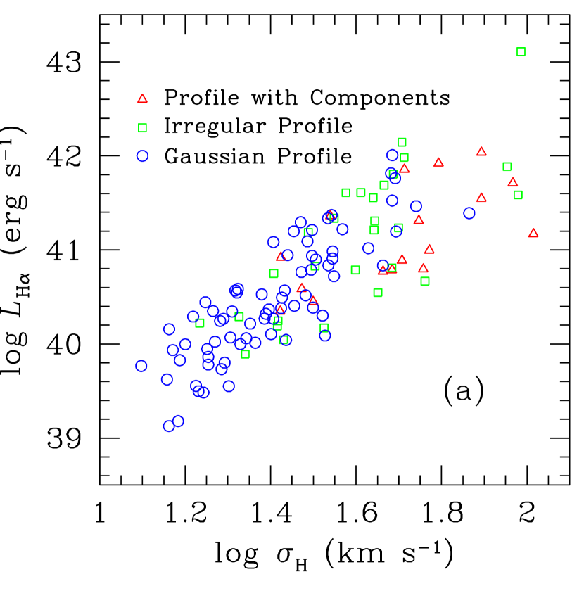
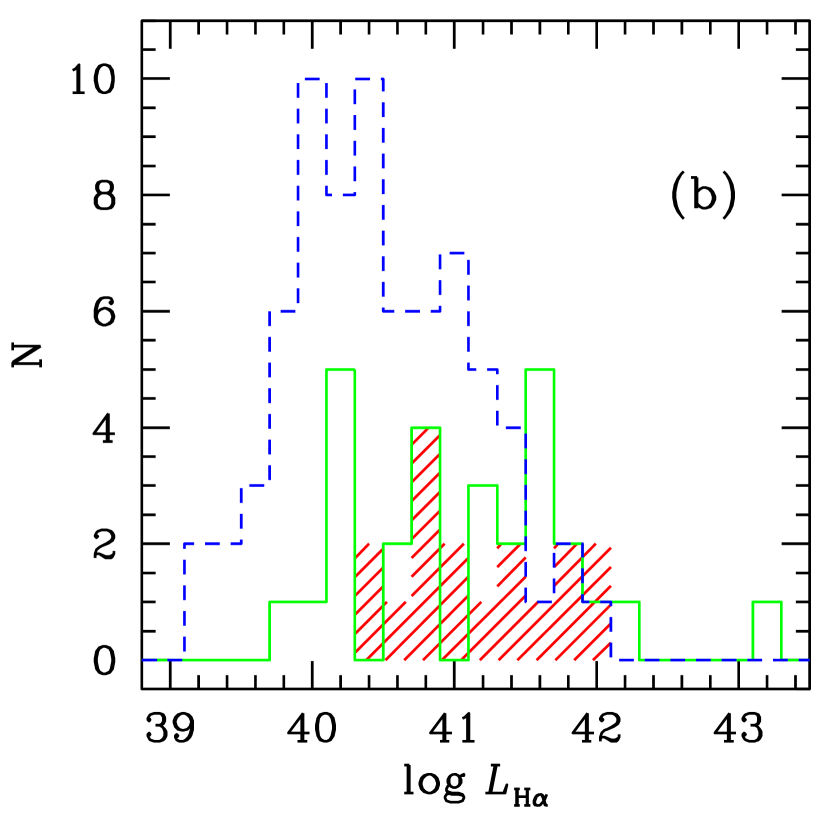
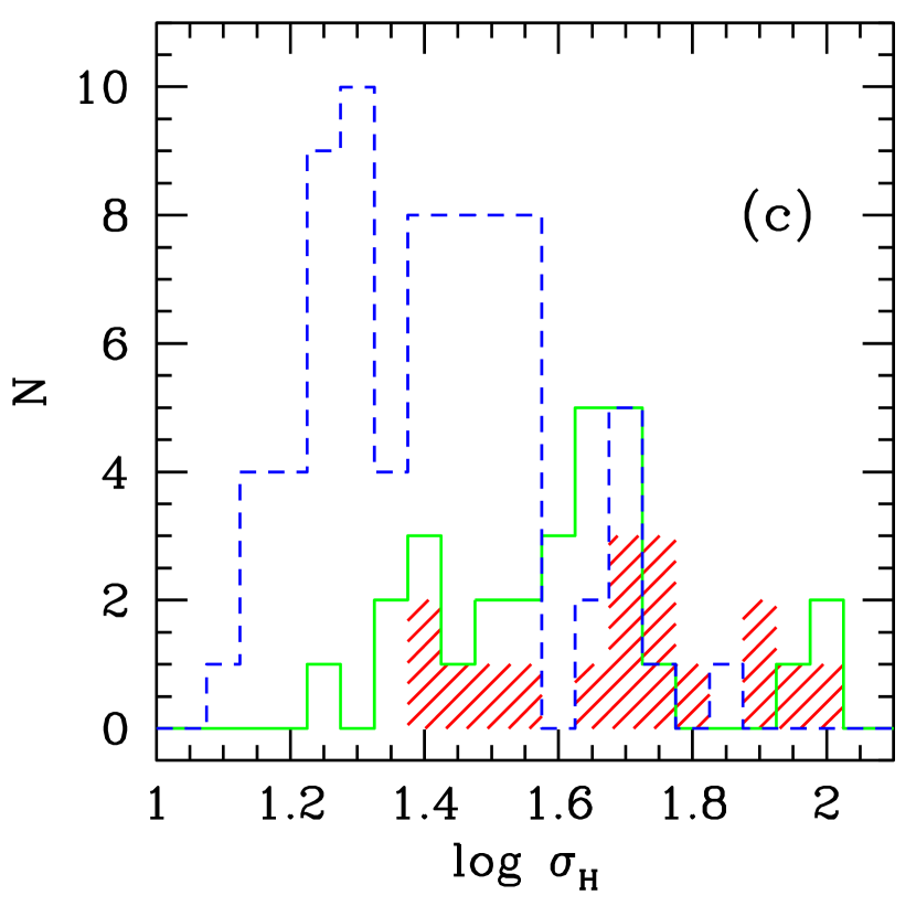
Figure 6: (a) The $L_{\scriptsize\mbox{H}\alpha}$-$\sigma_{\scriptsize\mbox{H}}$ for 117 galaxies with spectrophotometry obtained; (b) the luminosity distribution; and (c) the velocity dispersion distribution. The colour codes for each class of galaxy, (G, I and C) are as given in the label of plot (a).

In order to minimize the uncertainties due to a heterogeneous data set, we further analyze the $L$-$\sigma$ relation for those galaxies that have line-widths measured from FEROS data and spectrophotometry compiled from KTC’s work. An additional 4 objects (UM 382, CTS 1027, II Zw 70 and Tol 2138-405) that have good new spectrophotometry are included.

Figure 7 shows the $L$-$\sigma$ relation for the homogeneous sample described above including galaxies with close to Gaussian emission line profiles (81 objects). The regression fits for the total sample and only for the G subsample (53 objects) are presented in Table 6. The class of ordinary least-square fits (OLS) used in this work is appropriate to problems where the intrinsic scatter dominates the errors arising from the measurement process (Isobe et al., 1990). We argue that the OLS(Y$|$X) is the most appropriate to describe the $L$-$\sigma$ relation for our data set and is the best to be compared with previous calibrations (MTM, Telles et al., 2001). A second point is that the uncertainties in $\sigma$ are much smaller than in luminosity, which justify the first to be treated as an independent parameter in a direct linear regression. Nevertheless the other fits give us an idea of maximum limits of the regression coefficients (slope and zero point).

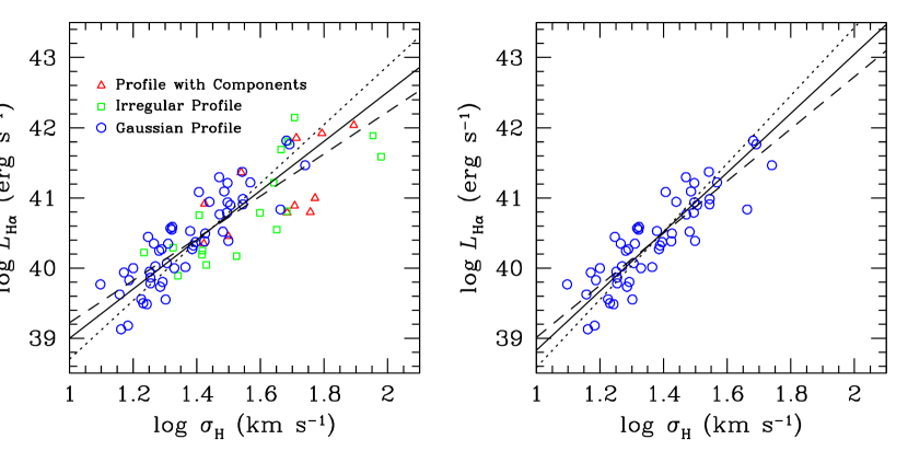
Figure 7: The $L_{\scriptsize\mbox{H}\alpha}$-$\sigma_{\scriptsize\mbox{H}}$ relation for all galaxies with homogeneous spectrophotometry (81 objects G, I and C, left) and only for those showing regular Gaussian profiles (53 objects G, right). The dashed line represents OLS(Y$|$X), the dotted line represents OLS(X$|$Y) and the solid line represents the bisector fit. All regression coefficients are presented in Table 6.

It is clear that the $L$-$\sigma$ relation including only G galaxies is tighter and steeper than the one including the whole sample of HiiGs. It suggests that the Gaussianity of the emission line profiles in these systems may be associated with the nature of the $L$-$\sigma$ relation. Figure 8 shows the $W_{\scriptsize\mbox{H}\beta}$ distribution for each class G, I and C. Note that most G galaxies are concentrated in the region of high $W_{\scriptsize\mbox{H}\beta}$ ($>30$Å). Thus a sample selection criterion based on high $W_{\scriptsize\mbox{H}\beta}$ would be efficient to select also galaxies with the most Gaussian profiles. The consequences of this result to the nature of the $L$-$\sigma$ relation are profound. Since $W_{\scriptsize\mbox{H}\beta}$ is an age indicator of the current starburst, resultant Gaussian line profiles may be associated with the youngest systems. If the $L$-$\sigma$ relation for HiiGs has in fact an upper envelope described by those galaxies with zero-age and maximum $W_{\scriptsize\mbox{H}\beta}$ values, it should be populated only by HiiGs showing the most Gaussian line profiles. In Section 4.2 we will be more rigorous in selecting a subsample of G galaxies with the most Gaussian line profiles by a semi-quantitative criterion in order to investigate if it has additional consequences on the slope and scatter of the $L$-$\sigma$ relation.

Table 6: Regressions for log $L_{\scriptsize\mbox{H}\alpha}$ versus log $\sigma_{\scriptsize\mbox{H}}$.

Linear Regression	Intercept	Slope	RMS
	(A)	(B)
All galaxies (81 objects)
Pearson correlation coefficient ($r$) = 0.85
	log $L$ = A + B $\times$ log $\sigma$
OLS(Y$|$X) …………..	36.21 $\pm$ 0.32	3.01 $\pm$ 0.23	0.37
OLS(X$|$Y) …………..	34.52 $\pm$ 0.38	4.18 $\pm$ 0.27
OLS Bisector ………	35.49 $\pm$ 0.32	3.51 $\pm$ 0.23
Galaxies with Gaussian profiles (53 objects)
$r$ = 0.88
OLS(Y$|$X) …………..	35.29 $\pm$ 0.42	3.72 $\pm$ 0.31	0.31
OLS(X$|$Y) …………..	33.73 $\pm$ 0.47	4.85 $\pm$ 0.34
OLS Bisector ………	34.61 $\pm$ 0.41	4.22 $\pm$ 0.30
More restrictive subsample (37 objects)
$r$ = 0.90
OLS(Y$|$X) …………..	34.80 $\pm$ 0.41	4.14 $\pm$ 0.29	0.29
OLS(X$|$Y) …………..	33.45 $\pm$ 0.53	5.13 $\pm$ 0.38
OLS Bisector ………	34.19 $\pm$ 0.43	4.58 $\pm$ 0.30

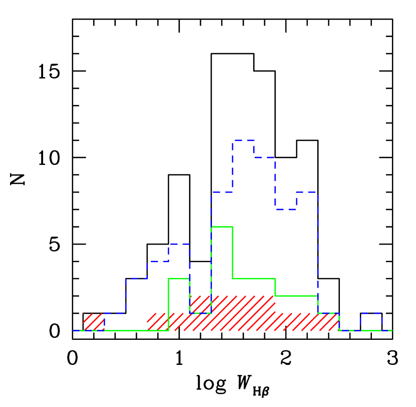
Figure 8: The H$\beta$ equivalent width distributions (in log) for each class of galaxies namely G (53), I (17) and C (11) presented in Figure 7. The solid line represents the distribution including all subsamples (81).

4 Data Analysis

4.1 Aperture Effects

The $L$-$\sigma$ relation may be in principle affected by the aperture effect in two ways. Firstly, if the observation comes from fixed-slit spectroscopy ($\sim$ 2″) as in this work, nearby objects should have their fluxes underestimated and hence their luminosities too. Furthermore, extended and more compact objects, both at the same distance, may suffer differentially from this effect. It may also have implications in determining their physical conditions (Kewley et al., 2005). An aperture correction factor may be applied to our calibration by using the available data in Lagos et al. (2007). They observed a sample of HiiGs with H$\beta$ narrow band imaging and analyzed the surface photometry as compared with the spectrophotometry of Kehrig et al. (2004). Many of the galaxies in their sample are also part of our present sample. Taking into account the observational and calibration errors in their analysis, there is a constant offset of the order of the observational scatter in the comparison that can be added to our derived $L_{\scriptsize\mbox{spec}}$: $\Delta L_{\scriptsize\mbox{H}\beta}\sim 0.25$ with an RMS = 0.2, comparable to the RMS of our $L$-$\sigma$ relation. We have not done this a priori, since this correction would only introduce additional observational scatter, masking the contribution of the physical parameters in the analysis of the manifold of HiiGs. This effect is expected to be negligible for galaxies beyond $>100$ Mpc according to this analysis, and an improvement in this calibration will only come when this relation is verified for a sample of HiiGs beyond the local supercluster with new spectrophotometric data sets and new high resolution spectroscopy. We have also verified that a correlation of the narrow band surface photometry of the main star forming knot seems to be tighter than with the narrow band surface photometry of the integrated galaxy. This may be due to the mixed morphology of the galaxies as a function of luminosity (see Lagos et al., 2007; Telles et al., 1997), but also due to the very nature of the $L$-$\sigma$ relation, in the sense that it may be more closely related to the local gravitational potential of the starburst, rather than the global dynamics. The relation still holds for the determination of galactic masses if we assume that more massive galaxies host more massive starbursts in a homologous way. These issues remain to be investigated in more detail.

Multiplicity of star-forming regions and the aperture effect can also introduce a bias in $\sigma$ determination — a single observation integrates light from more than one starburst region in the same galaxy. This could introduce a systematic velocity component in the integrated line profiles since Super Star Clusters and their associated GHiiRs may present relative radial velocities that would add light in a non-trivial way. Although multiplicity does not necessarily preclude Gaussianity, it seems to be usually associated with asymmetric line profiles (Bordalo et al., 2009). We have also found very compact objects presenting line profiles with multiple components (e.g. CTS 1033 shown in Figure 9). However, most of the galaxies classified as C are not compact, but extended systems frequently associated to nuclear starburst galaxies, where the systemic rotational component dominates the features in emission line profiles.

The multiplicity effect seems to be inherent in the $L$-$\sigma$ relation causing no strong bias, otherwise the $L$-$\sigma$ relation would be not verified, even in the short redshift range of our sample. The physical sizes covered by the observations span from a few hundred parsecs in nearby objects (e.g. UM 461 and MRK 36), characterizing sizes of single GHiiRs, to a few kiloparsecs (e.g. CTS 1008 and Cam 08-28A). In addition, multiplicity and aperture effects can be greatly reduced by selecting only the galaxies showing the most Gaussian line profiles.

4.2 Gaussian Profile Galaxies

In order to find a more homogeneous sample and, in addition, test the visual classification presented in Section 3.1, we have further adopted a semi-quantitative criterion to search for galaxies with the most Gaussian emission line profiles. These seem to be the ones that show the lower scatter in the $L$-$\sigma$ plane, as suggested in Figure 7, and therefore deserve special attention. The quantitative estimators that we used were the skewness ($\xi$) and kurtosis ($\kappa$) of the emission line profiles (see Miesch, Scalo, & Bally, 1999, for the use of these estimators in one-point velocity statistics of star-forming regions). These estimators are related to the third ($m_{3}$) and fourth ($m_{4}$) moments of the distribution through the formulae

$$\xi=\frac{m_{3}}{s^{3}}$$

and

$$\kappa=\frac{m_{4}}{s^{4}},$$

where $s$ is the standard deviation of the distribution and $m_{3}$ and $m_{4}$ their higher moments. For practical cases concerning real data spectra, where $\lambda$ is the wavelength and $y$ is the flux, the formulae for these estimators can be written by:

$$\mbox{mean}=\mu=\frac{\sum\lambda\cdot y}{\sum y},$$

$$\mbox{standard deviation}=s=\sqrt{\frac{1}{\sum y}\sum(\lambda-\mu)^{2}\cdot y},$$

$$\mbox{skewness}=\xi=\frac{1}{\sum y}\frac{\sum(\lambda-\mu)^{3}\cdot y}{s^{3}},$$

$$\mbox{kurtosis}=\kappa=\frac{1}{\sum y}\frac{\sum(\lambda-\mu)^{4}\cdot y}{s^{4}}.$$

Before we proceed the calculation of $\xi$ and $\kappa$ estimators we smoothed all FEROS spectra with a box of 11 pixels (FEROS’s scale is 0.03Å/pix) using SPLOT. Since our aim was to estimate the global shape of the emission lines, the smooth procedure is very useful to eliminate high frequency noise. The most Gaussian profile galaxies were selected as the ones which met the criterion of symmetry: $\mid\xi\mid$ $<$ 0.1 and 2.9 $<$ $\kappa$ $<$ 3.1. The estimators were calculated in a window centered at the mean, obtained from the single Gaussian fit (centroid), and defined as the one in which the line intensity falls to 20% of its peak value. This methodology ensures that the estimators show a good consistency between them, however the size of integration window over $\lambda$ interval is somewhat a matter of definition which should be based on the quality of the data.

Figure 9: Examples of emission line profiles in linear-logarithmic axes. UM 463 (upper left) and [F80] 30 (upper right) met the criterion of symmetry described in the text (G^′), (bottom left) CTS 1033 was qualitatively visually rejected by presenting multiple components and (bottom right) II Zw 40 does not meet the symmetry criterion. Measurements of $\xi$ and $\kappa$ estimators are shown in each panel. Solid lines represent single Gaussian fits to the observed profiles (crosses).

Only FEROS galaxies with S/N in the line greater than 30 were analyzed by this method. Emission line profiles of 49 galaxies met the above criterion of symmetry. Two examples (UM463 and [F80] 30) are presented in Figure 9 (upper panels), including their shape estimators $\xi$ and $\kappa$. We also present the H$\alpha$ emission line profile of II Zw 40 ($\xi$=0.18, $\kappa$=3.05) as an example in which the criterion of symmetry was efficient to reject profiles with strong asymmetries (Figure 9 bottom right). Most estimators were calculated using the H$\alpha$ line and only few using [OIII] 5007Å due to the presence of bad pixels or significantly lower S/N in H$\alpha$. A comparison with the G subsample classified visually (Table 2) showed good agreement except for six galaxies that were previously classified as I or C, namely Tol 0104-388, Tol 0957-278, CTS 1030, CTS 1033, CTS 1037 and CTS 1039. These objects were thus visually rejected. We kept the visual classification for these galaxies since the first two objects present two intense components which are identified in the other emission lines observed, while CTS 1033 presents at least three emission components (Figure 9 bottom left). The last is a very special case in which asymmetries in the integration window are compensated resulting in estimators that mimic a symmetric profile ($\xi$=-0.04, $\kappa$=3.03). The other three objects present intense broad components not well evaluated in the integration window though they are symmetric. Thus 43 galaxies compose a more restrictive subsample of the galaxies showing the most Gaussian line profiles and they were assigned as G^′ in Table 2.

The need for a qualitative analysis of the emission line profiles is in fact a limitation of the method applied to our data. Since the S/N ratio is relatively low in the wings of the line, we need to limit the integration window to a fixed proportion of the peak value (see above), in order to keep the consistency between the values from very different S/N lines. Nevertheless, the method provides a way to determine a homogeneous sample of galaxies based on their kinematic properties.

Table 6 shows the regression fits for the $L$-$\sigma$ relation considering the more restrictive subsample G^′. From 43 objects identified as G^′, 37 had homogeneous observational data as described in Section 3.4 and were used to derive the calibration coefficients. Although this sample presents few objects in the range 1.6 $<$ $\log\sigma$ $<$ 1.8, the OLS fits show that the $L$-$\sigma$ is steeper than the one for the whole G subsample (53 objects). We conclude that the galaxies showing the most Gaussian line profiles show the $L$-$\sigma$ relation that could be identified as an upper envelope $L\propto\sigma^{4}$ with minimum scatter $\delta\log L_{\scriptsize\mbox{H}\alpha}=0.29$.

4.3 The Second Parameter

Terlevich & Melnick (1981) and Melnick et al. (1988) have suggested that the dependent parameter $L_{\scriptsize\mbox{Balmer}}$ can be predicted by $\sigma$ and O/H, which should define the manifold of HiiGs. Telles & Terlevich (1993) also showed that the structural parameter namely radius of the burst should be considered as a second parameter in $L$-$\sigma$, acting remarkably similarly to effective radius in the fundamental plane of elliptical galaxies. It is crucial to investigate the existence of an independent second parameter (or a third) in the $L$-$\sigma$ relation not only to obtain a precise distance indicator but also to understand the physics behind this scaling relation. If the underlying relation is in fact that between mass and luminosity, as proposed by these authors, then $\sigma$ can be used properly to obtain dynamical masses of these systems with great relevance for the high redshift studies of HiiGs counterparts, such as the Lyman Break Galaxies (Lowenthal et al., 2009, and references therein).

Table 7: Correlation Matrix.

PCA $L_{\scriptsize\mbox{H}\alpha}$, $\sigma_{\scriptsize\mbox{H}}$, O/H, $W_{\scriptsize\mbox{H}\beta}$ and [OIII]/[OII] (95 objects)
$\log$ $L_{\scriptsize\mbox{H}\alpha}$	1
$\log$ $\sigma_{\scriptsize\mbox{H}}$	0.82	1
$\log$ (O/H)	0.22	0.47	1
$\log$ $W_{\scriptsize\mbox{H}\beta}$	0.13	-0.15	-0.58	1
$\log$ [OIII]/[OII]	-0.03	-0.32	-0.69	0.86	1
	$\log$ $L_{\scriptsize\mbox{H}\alpha}$	$\log$ $\sigma_{\scriptsize\mbox{H}}$	$\log$ (O/H)	$\log$ $W_{\scriptsize\mbox{H}\beta}$	$\log$ [OIII]/[OII]

Table 8: Eigenvectors and eigenvalues.

	Principal component
	I	II	III
$\log$ $L_{\scriptsize\mbox{H}\alpha}$	0.39	-0.88	-0.11
$\log$ $\sigma_{\scriptsize\mbox{H}}$	0.66	-0.70	-0.08
$\log$ (O/H)	0.86	0.07	0.51
$\log$ $W_{\scriptsize\mbox{H}\beta}$	-0.77	-0.54	0.25
$\log$ [OIII]/[OII]	-0.88	-0.38	0.16
Eigenvalues	2.69	1.70	0.37
% variance	53.9%	34.0%	7.3%

We have used the Principal Component Analysis (PCA) to investigate the relative dependence of the $L$-$\sigma$ relation on a possible second parameter based on our new data set, following the early analysis by MTM. Let us first analyze the largest sample possible considering the 5 parameters (variables) — $L_{\scriptsize\mbox{H}\alpha}$, $\sigma_{\scriptsize\mbox{H}}$, O/H, $W_{\scriptsize\mbox{H}\beta}$ and [OIII]/[OII]. The sample includes $n=95$ objects with all these quantities known (Tables 3 and 5). All quantities were considered in logarithmic scales. Table 7 shows the lower half triangle of the correlation matrix. Visual analysis of Table 7 shows that strong correlations are found between $W_{\scriptsize\mbox{H}\beta}$ and [OIII]/[OII] ($r=0.86$) and $L_{\scriptsize\mbox{H}\alpha}$ and $\sigma_{\scriptsize\mbox{H}}$ ($r=0.82$). It is also worth noting that the correlations between $L_{\scriptsize\mbox{H}\alpha}$ and [OIII]/[OII], $L_{\scriptsize\mbox{H}\alpha}$ and $W_{\scriptsize\mbox{H}\beta}$ and $\sigma_{\scriptsize\mbox{H}}$ and $W_{\scriptsize\mbox{H}\beta}$ are near zero. The correlations of O/H and $W_{\scriptsize\mbox{H}\beta}$ and O/H and [OIII]/[OII] are negative, while O/H and $L_{\scriptsize\mbox{H}\alpha}$ and O/H and $\sigma_{\scriptsize\mbox{H}}$ are positive.

The first three principal components (PCs) with their loadings obtained from the correlation matrix, as well as the eigenvalues ($l$) and the respective individual percentages ($l/5$) of total variance (5) are presented in Table 8. Nearly 88% of the variance among the 95 sample points lies in only two dimensions. The number 2 of dimensions of the manifold can be easily verified due to the bimodal behavior of the variance (Jolliffe, 2002). The first two principal components (PCI and PCII) present eigenvalues well above 1 (or 1/5=20%), while the others lie well below this value. In addition, one can estimate the confidence interval for the eigenvalue 1 using the formula $\sqrt{2l^{2}/(n-1)}$ which provides $l=1.00\pm 0.15$ (or $20\pm 3\%$), showing that PCII with 34% and PCIII with 7.3% are far from $l=20\pm 3\%$. This test is justified since in PCA all variables have (0,1)-normalization, so any PC with an eigenvalue less than 1 is not worth consideration. This criterion to decide the dimensionality of the manifold on the space parameters, also called “eigenvalue-one”, has gained almost universal acceptance (see Brosche (1973) and Bujarrabal et al. (1981) for the earliest papers applying the PCA technique to galaxy samples).

Since PCI and PCII contain no more than 88% of the total variance and other PCs present very small eigenvalues, we show that the addition of O/H, $W_{\scriptsize\mbox{H}\beta}$ and [OIII]/[OII] does not contribute to explain the total variance of the space parameters and hence they can not be used simultaneously to reduce the scatter in the $L$-$\sigma$ relation. These three well known indicators of the physical conditions in star-forming regions are strongly correlated with each other and the correlations found here are in good agreement with early findings (e.g. Campbell et al., 1986). The interrelationships between them are known and of intense debate in literature (Terlevich et al., 2004; Hoyos & Díaz, 2006, and references therein). It introduces a problem commonly faced by the PCA technique and multiple regression known as collinearity (or multicollinearity). Multicollinearities are often indicated by large correlations between subsets of the variables which can be seen in the correlation matrix for variables O/H, $W_{\scriptsize\mbox{H}\beta}$ and [OIII]/[OII] (Table 7). These three parameters are the ones that have high loadings of PCI, hence they are variables which are most closely related to PCI (Table 8). On the other hand, the high loadings in PCII identify $L_{\scriptsize\mbox{H}\alpha}$ and $\sigma_{\scriptsize\mbox{H}}$ as the parameters most closely related to PCII.

The main result of the above analysis is that PCI can be thought as a measure of physical conditions in HiiGs, whereas PCII is a measure of the strength of the $L$-$\sigma$ relation. Note that we do not invoke any prior knowledge about the physical origin of the $L$-$\sigma$ relation. As PCs are pairwise uncorrelated, the conclusion is that physical conditions are responsible for part of the observed scatter in the $L$-$\sigma$ relation, though the three parameters studied here can not be used simultaneously to explain that. Note that $\sigma_{\scriptsize\mbox{H}}$ presents its highest loading in PCII, which suggests that it is not a primary consequence of internal physical conditions (measured by these three parameters), and is possibly not controlled by subsequent mechanical feedback processes due to massive stellar evolution. However, the weaker but real correlation between $\sigma_{\scriptsize\mbox{H}}$ and O/H ($r=0.47$, see Table 7) is responsible for the non-negligible loading for $\sigma_{\scriptsize\mbox{H}}$ in PCI (0.66). It shows that O/H introduces some degree of multicollinearity as an additional independent parameter in the $L$-$\sigma$ relation. Although a high degree of multicollinearity does not violate the assumptions of the regression model, it influences the variance of the estimated regression coefficients (partial slopes and intercept). We will present the $\sigma$-$Z$ relation in the context of the discussion about the internal dynamics of HiiGs in Section 5.1.

For now, we are not interested in fully predicting the dependent variable $L_{\scriptsize\mbox{H}\alpha}$ based on the other parameters studied here. They present a high degree of multicollinearity mainly due to the $W_{\scriptsize\mbox{H}\beta}$-[OIII]/[OII] relation. Instead, we want to identify which physical condition parameter explains more efficiently the scatter as a second independent parameter in the $L$-$\sigma$ relation. A possible way to further investigate the variance of the space parameters, overcoming the problem of multicollinearity in PCA, is by using only a subset of parameters, where the subset is chosen so that it does not contain or it is intended to minimize multicollinearities.

Table 9 presents the results of the PCA table for the same previous sample containing 95 objects, undistinguished by their emission line profiles or $W_{\scriptsize\mbox{H}\beta}$, for the three parameter spaces: [$L_{\scriptsize\mbox{H}\alpha}$,$\sigma_{\scriptsize\mbox{H}}$,O/H], [$L_{\scriptsize\mbox{H}\alpha}$,$\sigma_{\scriptsize\mbox{H}}$,$W_{\scriptsize\mbox{H}\beta}$] and [$L_{\scriptsize\mbox{H}\alpha}$,$\sigma_{\scriptsize\mbox{H}}$,[OIII]/[OII]]. The results for [$L_{\scriptsize\mbox{H}\alpha}$,$\sigma_{\scriptsize\mbox{H}}$,O/H] show that in addition to $L_{\scriptsize\mbox{H}\alpha}$ and $\sigma_{\scriptsize\mbox{H}}$, O/H has a relatively high loading in the PCI (0.61), which shows its strong relevance to explain the variance in the PCI. It results from the relatively higher correlation of O/H with $\sigma_{\scriptsize\mbox{H}}$ as mentioned above. Therefore PCII only explains 27% of the total variance. On the other hand, the analysis with the subset [$L_{\scriptsize\mbox{H}\alpha}$,$\sigma_{\scriptsize\mbox{H}}$,$W_{\scriptsize\mbox{H}\beta}$] shows that $W_{\scriptsize\mbox{H}\beta}$ is uncorrelated with $\sigma_{\scriptsize\mbox{H}}$ and contributes efficiently to explain 35% of the variance in the PCII. The ionization ratio [OIII]/[OII] also presents a higher contribution to PCII than O/H.

Table 9: Testing the second parameter through individual principal component analysis - 95 objects undistinguished by their emission line profiles.

	Principal Component
Parameter	I	II	III
$\log$ $L_{\scriptsize\mbox{H}\alpha}$	0.88	-0.42	0.23
$\log$ $\sigma_{\scriptsize\mbox{H}}$	0.96	-0.12	-0.27
$\log$ (O/H)	0.61	0.79	0.09
Eigenvalues	68.5%	27.0%	4.5%
$\log$ $L_{\scriptsize\mbox{H}\alpha}$	0.95	0.18	-0.25
$\log$ $\sigma_{\scriptsize\mbox{H}}$	0.96	-0.15	0.25
$\log$ $W_{\scriptsize\mbox{H}\beta}$	-0.03	0.99	0.08
Eigenvalues	60.8%	34.9%	4.3%
$\log$ $L_{\scriptsize\mbox{H}\alpha}$	-0.90	-0.36	0.24
$\log$ $\sigma_{\scriptsize\mbox{H}}$	-0.97	-0.03	-0.25
$\log$ [OIII]/[OII]	0.38	-0.92	-0.08
Eigenvalues	63.2%	32.6%	4.2%

The residual variance of 4-5% in PCIII (Table 9) accounts for observational errors, but a fraction of it can be explained by the fact that we have analyzed a heterogeneous sample. We have not distinguished galaxies by their emission line profiles. In fact, part of the large scatter in the high $L$ and $\sigma$ regime populated mostly by I and C galaxies (see Figure 6) may not be explained at all, since single Gaussian fits seem not to well represent the internal kinematics in these systems or the resultant line widths are not well correlated with $L$. In addition, there must be outliers also due to photometric errors propagated to parameters that may be perturbing the PCA results. PCA is a powerful technique that can be also used to detect outliers in data sets providing robust results. In order to obtain the distance estimators presented in next section, we have investigated and detected outliers in the context of multiple regression.

We conclude by saying that $W_{\scriptsize\mbox{H}\beta}$ as an age estimator of the starburst in HiiGs can not be neglected in a regression model in order to obtain a distance indicator based on the $L$-$\sigma$ relation. The ionization ratio [OIII]/[OII] acts in a similar way as $W_{\scriptsize\mbox{H}\beta}$ and can be explicitly considered in the absence of $W_{\scriptsize\mbox{H}\beta}$. Finally, the results shown above do not mean that O/H can not be used as a second parameter, instead we have verified that its efficiency to reduce the scatter of the $L$-$\sigma$ relation may be real but it seems to be smaller than the one using $W_{\scriptsize\mbox{H}\beta}$. Additionally, O/H introduces a higher degree of collinearity due to its relationship with $\sigma$.

4.4 Empirical Relations

Primary luminosity dependence on $\sigma$ has been evaluated by the $L$-$\sigma$ relation considering only galaxies showing nearly Gaussian emission line profiles. For a given velocity dispersion $\sigma$ and metallicity (O/H), the galaxies with the largest H$\beta$ equivalent width $W_{\scriptsize\mbox{H}\beta}$ or ionization ratio [OIII]/[OII] should present also the largest Balmer luminosities $L_{\scriptsize\mbox{H}\alpha}$. On the other hand, for a given $\sigma$ and $W_{\scriptsize\mbox{H}\beta}$ or [OIII]/[OII], galaxies with the lowest O/H ratio should also present the largest $L_{\scriptsize\mbox{H}\alpha}$. The results found here for the $L$-$\sigma$ relation (Table 6) and PCA (Section 4.3), as well as in early studies (Terlevich & Melnick, 1981, MTM), corroborate the same empirical model for HiiGs. Therefore, we need to obtain precise regression coefficients through multiple regressions.

Table 10: Multiple regressions for $L_{\scriptsize\mbox{H}\alpha}$, $\sigma_{\scriptsize\mbox{H}}$, O/H, $W_{\scriptsize\mbox{H}\beta}$ and [OIII]/[OII].

Parameters	Regressions for $\log L_{\scriptsize\mbox{H}\alpha}$	RMS
Galaxies with Gaussian profiles (53 objects1)
$L$-$\sigma$ …………………….	(35.29$\pm$0.42) + (3.72$\pm$0.31)log $\sigma$	0.312
$L$-$\sigma$-O/H ……………..	(38.22$\pm$1.02) + (4.19$\pm$0.31)log $\sigma$ $-$ (0.44$\pm$0.14)log(O/H)	0.289
$L$-$\sigma$-$W_{\scriptsize\mbox{H}\beta}$ …………….	(34.60$\pm$0.39) + (3.84$\pm$0.25)log $\sigma$ + (0.32$\pm$0.08)log $W_{\scriptsize\mbox{H}\beta}$	0.274
$L$-$\sigma$-[OIII]/[OII] ……	(34.69$\pm$0.38) + (4.06$\pm$0.27)log $\sigma$ + (0.34$\pm$0.09)log [OIII]/[OII]	0.275
$L$-$\sigma$-O/H-$W_{\scriptsize\mbox{H}\beta}$ ……..	(35.63$\pm$1.43) + (3.96$\pm$0.31)log $\sigma$ $-$ (0.14$\pm$0.18)log(O/H) + (0.27$\pm$0.11)log $W_{\scriptsize\mbox{H}\beta}$	0.275
$L$-$\sigma$-O/H-[OIII]/[OII]	(35.95$\pm$1.01) + (4.17$\pm$0.22)log $\sigma$ $-$ (0.17$\pm$0.17)log(O/H) + (0.27$\pm$0.11)log [OIII]/[OII]	0.275

Parameters	Regressions for $\log L_{\scriptsize\mbox{H}\alpha}$	RMS
Galaxies with Gaussian profiles (45 objects) without outliers.
$L$-$\sigma$ …………………….	(35.26$\pm$0.38) + (3.76$\pm$0.27)log $\sigma$	0.270
$L$-$\sigma$-O/H ……………..	(39.94$\pm$0.99) + (4.33$\pm$0.25)log $\sigma$ $-$ (0.68$\pm$0.14)log(O/H)	0.217
$L$-$\sigma$-$W_{\scriptsize\mbox{H}\beta}$ …………….	(34.58$\pm$0.30) + (3.78$\pm$0.20)log $\sigma$ + (0.39$\pm$0.06)log $W_{\scriptsize\mbox{H}\beta}$	0.201
$L$-$\sigma$-[OIII]/[OII] ……	(34.64$\pm$0.30) + (4.09$\pm$0.21)log $\sigma$ + (0.39$\pm$0.07)log [OIII]/[OII]	0.204
$L$-$\sigma$-O/H-$W_{\scriptsize\mbox{H}\beta}$ ……..	(36.64$\pm$1.38) + (4.01$\pm$0.25)log $\sigma$ $-$ (0.27$\pm$0.18)log(O/H) + (0.29$\pm$0.09)log $W_{\scriptsize\mbox{H}\beta}$	0.197
$L$-$\sigma$-O/H-[OIII]/[OII]	(37.04$\pm$1.29) + (4.26$\pm$0.22)log $\sigma$ $-$ (0.32$\pm$0.17)log(O/H) + (0.28$\pm$0.09)log [OIII]/[OII]	0.198

1.- The same subsample with 53 G objects used in Table 6.

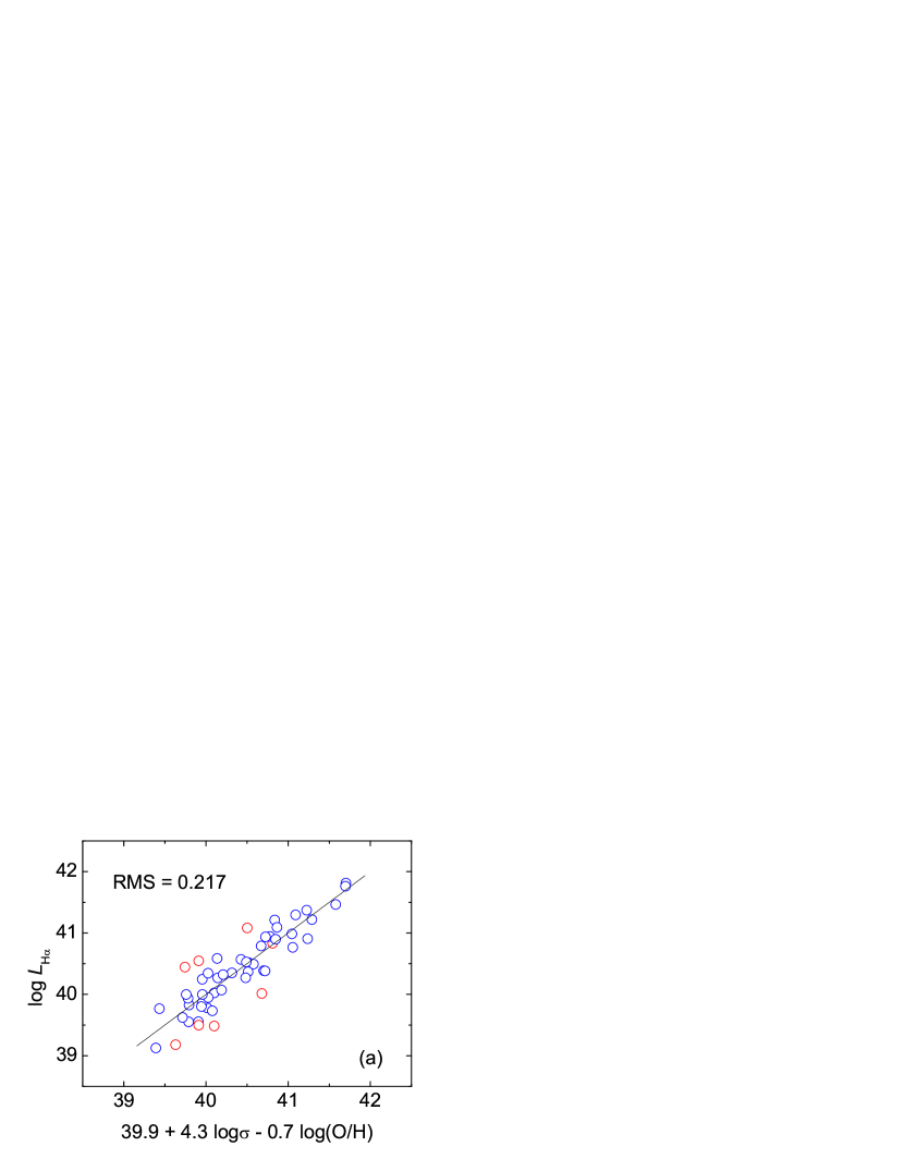
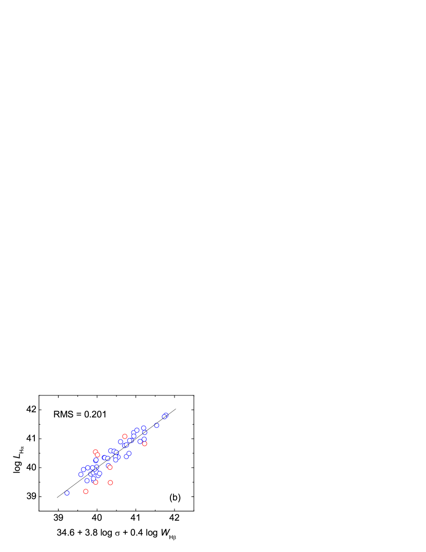
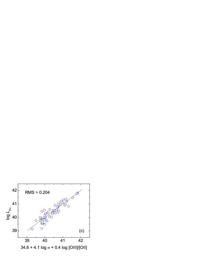
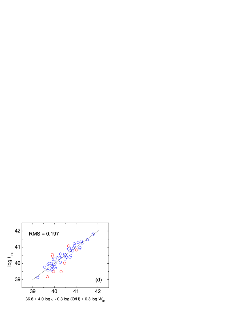
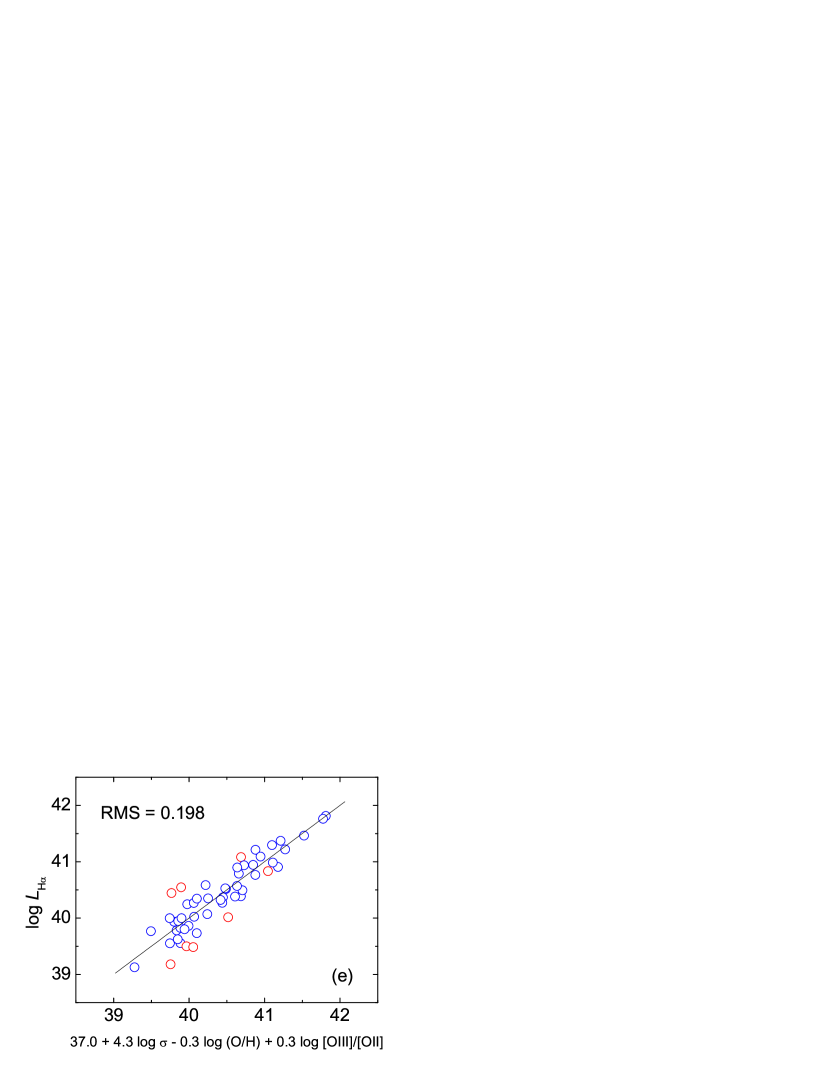
Figure 10: Regression models plotted against observed H$\alpha$ luminosities for 53 objects. The functional forms are presented in the $x$ axis of each graph. The solid lines represent the 1 to 1 lines fitted to the data. The calibration galaxies are plotted as open blue circles, whereas the outliers are plotted as open red circles.

Figure 11: Histograms for all parameters in the calibration sample (45 objects) in logarithmic units. Mean ($\mu$) and standard deviations ($s$) of the distributions are shown in each plot.

Let us derive a set of empirical relations that can provide distance indicators based on the homogeneous subsample of 53 objects showing nearly Gaussian line profiles (visually classified as G) that have shown the tightest $L$-$\sigma$ relation (Table 6). It is possible that some I or even C galaxies would fit in a regression model increasing the statistical significance of the regression coefficients, but in general, as shown in Section 3.4, they contribute to flatten the $L$-$\sigma$ relation increasing its scatter especially in the regime of high $L$ and $\sigma$ values. It suggests that some of them do not share the same physical properties as most of the G galaxies or the single fit procedure to derive their resultant $\sigma$ is not appropriate. These objects may also suffer differentially from aperture effects (Section 4.1). The sample containing 53 objects was chosen instead of the more restrictive one (37 objects), selected by the semi-quantitative criterion (Section 4.2), since the later are not well represented in the range 1.6 $<$ $\log\sigma$ $<$ 1.8 km s^-1.

Multiple regression fits for 53 objects are shown in Table 4.4. Linear fits to the $L$-$\sigma$ relation for the same sample were also presented in Table 6. Note that the scatter given by the RMS of the multiple regression fits did not reduce significantly by the inclusion of a second or a third independent parameter. It is mainly due to the presence of outliers. Outliers may not introduce a significant problem in the $L$-$\sigma$ relation (shown in Figure 7 and Table 6) because $L$ and $\sigma$ outlying measurements do not surpass the intrinsic scatter (RMS $\sim$ 0.30). We have included O/H, $W_{\scriptsize\mbox{H}\beta}$ and [OIII]/[OII], each carrying a potential source of error. Some data were in fact compiled from different works and they may have not been obtained at exact same region in the galaxies. A specialized statistics used to detect outliers in the context of multiple regressions is through the computation of leverage, discrepancy (studentized residual) and influence indices (Cook’s $D$). Conceptually, influence represents the product of leverage and discrepancy. These are known as the three characteristics of potentially errant data points (see Cohen et al., 2003, for a didactic presentation and concepts). Using this methodology eight data points were deleted from the sample containing 53 objects. We have verified that the presence of these outliers is mainly due to inclusion of objects with an uncertain nature (MRK 1201 and MRK 1318), with data considered from different sources (Tol 1008-286 and UM 463), and unusually high uncertainties in derived parameters due to low S/N spectra (UM 417, Tol 0505-387, UM 559 and Tol 2138-397). Thus, Table 4.4 also shows a set of empirical relations based on a sample of 45 objects without outliers. For RMS comparison with the ones from regression models with two or three independent parameters, we also presented the linear fit OLS(Y$|$X) to $L$-$\sigma$ relation for the sample containing 45 objects free from outliers. We reproduced a new version of the early empirical model $L$-$\sigma$-O/H used by MTM to derive their distance indicator with the same RMS scatter of $\delta\log L_{\scriptsize\mbox{H}\alpha}=0.22$. Independent functional forms for $L$-$\sigma$-$W_{\scriptsize\mbox{H}\beta}$ and $L$-$\sigma$-[OIII]/[OII] produce virtually the same result and they are both more efficient than O/H as a second independent parameter in the $L$-$\sigma$ relation reducing the RMS scatter to $\delta\log L_{\scriptsize\mbox{H}\alpha}=0.20$. In addition, we present the “true” empirical model for HiiGs, $L$-$\sigma$-O/H-$W_{\scriptsize\mbox{H}\beta}$ (R1) and $L$-$\sigma$-O/H-[OIII]/[OII] (R2).The scatter has not reduced significantly by the inclusion of a third independent parameter — O/H in $L$-$\sigma$-$W_{\scriptsize\mbox{H}\beta}\sim 2\%$ and O/H in $L$-$\sigma$-[OIII]/[OII] $\sim 3\%$ — but the residual is compatible with the expected error in luminosity, which prevents us from determining what fraction is intrinsic.

It is an important result that $W_{\scriptsize\mbox{H}\beta}$ can account alone for a significant fraction of the scatter in the $L$-$\sigma$ relation ($\sim 25\%$) with a minimum degree of collinearity. $W_{\scriptsize\mbox{H}\beta}$ has the advantage of being a simpler parameter to obtain from the spectra, though it depends on continuum detection. Alternatively, if the intense [OIII]$\lambda\lambda$4959, 5007 and [OII]$\lambda$3727 lines are detected one can use, with the same precision, the $L$-$\sigma$-[OIII]/[OII] regression model. On the other hand, the $L$-$\sigma$-O/H empirical model as distance indicator would be more difficult to apply at great distances, since it requires the detection of the [OIII]$\lambda 4363$ auroral line to precisely calculate oxygen abundances by the $T_{e}$-method.

Figure 10 presents all five regression models, including those with two (a, b and c panels) and three (d and e panels) independent parameters plotted against the observed $L_{\scriptsize\mbox{H}\alpha}$. The outliers are plotted as open red circles in all panels. Their predicted luminosity values were computed from the respective regression models for 45 objects presented in Table 4.4. Figure 11 presents the histograms of all five parameters used in regression models, $L_{\scriptsize\mbox{H}\alpha}$ (a), $\sigma_{\scriptsize\mbox{H}}$ (b), O/H (c), $W_{\scriptsize\mbox{H}\beta}$ (d) and [OIII]/[OII] (e), with their mean values and standard deviation in logarithmic units. These histograms characterize our calibration sample. Note that we have included some galaxies with $W_{\scriptsize\mbox{H}\beta}<30$Å in our sample, which were not included by MTM in their calibration sample. Our calibration sample with 45 local objects is a good representative sample of HiiGs in general. The mean, standard deviation and median (8.03) of the distribution of metallicity (Figure 11 panel c) are consistent with studies that characterize the population of HiiGs from much larger samples (Kniazev et al., 2004).

5 Discussion

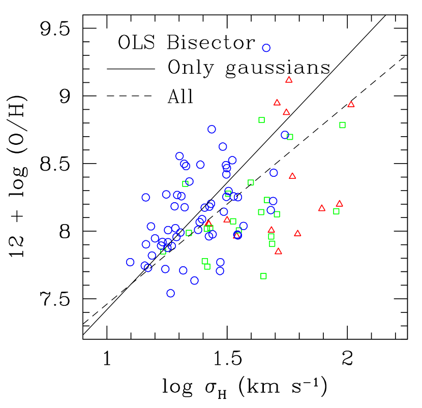
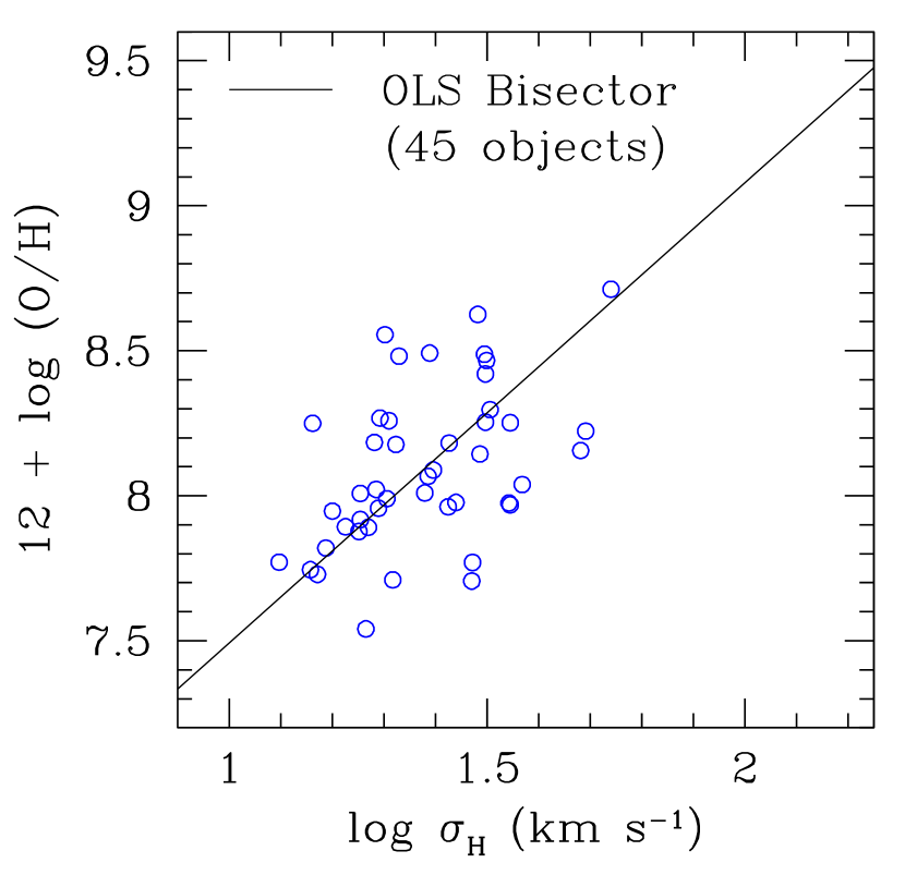
Figure 12: (left panel) The $\sigma$-$Z$ relation presented by 95 objects included in PCA. The solid and dashed lines represent the OLS bisector fits to the entire sample, $12+\log$(O/H)$=(5.98\pm 0.19)+(1.48\pm 0.14)\log\sigma_{\scriptsize\mbox{H}}$, and to the G sample, $12+\log$(O/H)$=(5.54\pm 0.34)+(1.88\pm 0.26)\log\sigma_{\scriptsize\mbox{H}}$, 60 objects), respectively. (right panel) The $\sigma$-$Z$ relation for the 45 objects used in the calibration sample without outliers (Table 4.4). The solid line represents the OLS bisector fit, $12+\log$(O/H)$=(5.91\pm 0.23)+(1.59\pm 0.17)\log\sigma_{\scriptsize\mbox{H}}$.

5.1 Internal Dynamics

The existence of the $L$-$\sigma$ relation for GHiiRs and HiiGs poses an intriguing question about the origin of the supersonic velocity widths of the emission line profiles. Several works have tried to answer this question through different approaches, but the hypothesis that these systems are gravitationally bound at least in the early stages of their evolution persists as a paradigm (Terlevich & Melnick, 1981). Figure 12 presents the $\sigma$-$Z$ relation for the whole sample presented in PCA (Section 4.3, 95 objects) and for those galaxies presented in the calibration sample (Section 4.4, 45 objects). If $\sigma$ correlates with metallicity in a similar manner as in gravitationally bound systems, the underlying relation could be the one between mass and metallicity. We present the bisector regression fits for different samples in the caption of Figure 12. In a recent work considering a large sample of HiiGs, Salzer et al. (2005) have shown the existence of the $L$-$Z$ relation for these systems. The Near-infrared (NIR) $L^{0.20}\propto Z$ relation found by the authors, which more directly reflects the underlying relationship between mass and metallicity, could be compared with our results in order to check whether the gravitational interpretation of the $L$-$\sigma$ relation of HiiGs is acceptable. However, the NIR luminosity comes mostly from the old stellar population, which may not be directly associated with the current mass of the starburst. Another option would be to compare the B band $L$-$Z$ with our $Z$-$\sigma$ relation. In fact, if we use the scaling relation $L^{0.28}\propto Z$ derived for the B band by Salzer et al. (2005) and consider the $Z\propto\sigma^{1.6}$ found here, we get closer to the $L\propto\sigma^{4}$. It still can not constrain much about the gravitational interpretation, since we have to explain how $\sigma$ of gas from the current starburst correlates with metallicity. A simple explanation would be that metal rich galaxies produce more massive starbursts, and this should be verified by observations. These interesting questions are above the scope of this work and should be further investigated.

Figure 13: Comparison between $\sigma$ derived from H$\beta$ and [OIII]$\lambda$4959. (left panel) All galaxies included. (right panel) Only galaxies presenting $\delta\sigma<2$ km s^-1. A small systematic difference $\sigma_{\scriptsize\mbox{H}}-\sigma_{\scriptsize\mbox{[OIII]}}=1-2$ km s^-1 is verified for galaxies with $\sigma\lesssim 60$ km s^-1.

Another hint about the origin of velocity widths found in HiiGs is provided by the systematic difference found between the width of Hii and [OIII] lines. This difference was firstly found in GHiiRs by Hippelein (1986). Figure 13 shows the differences found for our sample of HiiGs. In the left panel of Figure 13 we plot all galaxies with two lines observed, H$\beta$ and [OIII] 4959Å, whereas in the right panel we only plot the lines with the highest S/N with the smallest $\sigma$ errors ($\delta\sigma<1.2$ km s^-1). We do not see any systematic difference between these measurements above $\sim 50$ km s^-1. In fact, we note high discrepancies (5-20 km s^-1) between $\sigma_{\scriptsize\mbox{H}}$ and $\sigma_{\scriptsize\mbox{[OIII]}}$ with no trend. On the other hand, we see that HiiGs showing $\sigma$ values in the regime $15<\sigma<50$ km s^-1 present the intrinsic kinematic property also found in GHiiRs. There is a small systematic difference between $\sigma$ derived from both ions, $\langle\sigma_{\scriptsize\mbox{H}}-\sigma_{\scriptsize\mbox{[OIII]}}\rangle=1-2$ km s^-1. It seems to be a special consequence of coupled kinematic and physical conditions in these systems. A possible explanation would be the existence of a well behaved ionization structure, in which more excited ions are concentrated closer to the ionizing sources and densest regions. However a gradient of velocity dispersion is not observed at scales of tens to hundreds of parsecs in giant Hii regions. Other kinematic mechanisms that can be invoked to account for the observed systematic difference can be associated with turbulence (Hippelein, 1986).

We note that many HiiGs presented in the Figure 13 (right panel) are in fact those classified as Gaussian line profiles (open circles). It is another indication that these systems define a homogeneous sample in terms of their internal kinematics. Although our sample presents few galaxies with both measurements in high $\sigma$ regime, Figure 13 (left panel) suggests that HiiGs with $\sigma>$ 60 km s^-1 do not seem to share the same kinematic properties as the ones with $\sigma<$ 60 km s^-1.

5.2 Age Effects: Short- and Long-Term Evolution

We have shown that the age effect (short-term evolution) is the first order effect over the $L$-$\sigma$ relation and should not be neglected explicitly in an empirical relation in order to derive a distance indicator. Here we have tested $W_{\scriptsize\mbox{H}\beta}$ and [OIII]/[OII] as fiducial chronometers of the starburst. Both are virtually equally efficient in order to explain the scatter in the $L$-$\sigma$ plane. In order to reduce the scatter due to an age effect, one does not need a parameter that measures the burst age, but that measures efficiently the luminosity variation of the starburst as it ages. Photoionized models have shown that the most robust parameter to measure the luminosity evolution of the starburst is in fact $W_{\scriptsize\mbox{H}\beta}$ (Stasińska & Leitherer, 1996; Martín-Manjón et al., 2008). Its advantage is due to its weak dependence on the metallicity. [OIII]/[OII] and $W_{\scriptsize\mbox{[OIII]}5007}$ are more sensitive to metallicity. Figure 14 shows the predictions from photoionized models by Stasińska & Leitherer (1996) for H$\beta$ luminosity evolution of the starburst as a function of $W_{\scriptsize\mbox{H}\beta}$ (panels b and d) and [OIII]/[OII] (panels a and c), for a given starburst mass of 10⁶M_⊙ and two metallicities $12+\log$(O/H)=7.93 (panels a and b) and 8.33 (c and d). It is possible to see that $L$($W_{\scriptsize\mbox{H}\beta}$) presents nearly constant curve shape in both abundance sets, whereas $L$([OIII]/[OII]) does not present a monotonic curve in $12+\log$(O/H)=8.33 set, especially in the first 5 Myrs of the starburst. Note that $L$($W_{\scriptsize\mbox{H}\beta}$) still presents a more stable curve for $\log W_{\scriptsize\mbox{H}\beta}>1.5$ or $\sim$ 30Å. Models considering the continuous burst scenario have shown that $W_{\scriptsize\mbox{H}\beta}$ is in fact a robust age indicator of the starburst even for a significant presence of an underlying stellar population (Martín-Manjón et al., 2008).

Figure 14: H$\beta$ luminosity as a function of the [OIII]$\lambda 5007$/[OII]$\lambda 3727$ (a and c panels) and H$\beta$ equivalent width (b and d) in logarithmic units as predicted by single stellar population models by Stasińska & Leitherer (1996) with $M=10^{6}M_{\odot}$ and two metallicities, 12 + $\log$ (O/H) = 7.93 (a and b panels) and 8.33 (c and d panels). Numbers indicate the age of the starburst in Myr. Vertical dotted lines in panels b and d indicate the cutoff value $W_{\scriptsize\mbox{H}\beta}\sim 30$Å which coincides with age $\sim$ 5 Myr of the starburst in both models.

Metallicity itself is also a tracer of the evolution, though it is more closely linked to the long-term history of the star formation of the galaxy. The metallicity given by the O/H ratio, as proposed by MTM, may represent a second parameter in the $L$-$\sigma$ relation, since successive chemical enrichment promoted by generations of stars may affect globally the luminosity evolution (short-term) of each starburst.

Recent efforts have been made by Plionis et al. (2010) in order to investigate the precision required on distance determinations of high-$z$ HiiGs to achieve cosmological goals. Following Melnick et al. (2000), these authors propose to apply the scaling relations, like the ones derived here, to measure the dark energy equation of state, $w$($z$), and the matter content of the Universe $\Omega_{\scriptsize\mbox{m}}$, by using the Hubble diagram for HiiGs as an alternative to Supernovae type Ia above $z\sim 1$. Considerations made here about the systematic effects over the $L$-$\sigma$ relation may be valuable for its further application.

6 Summary

We have presented a new large data set of line width measurements for star-forming regions in over 100 HiiGs. This was used to analyse in some detail, the line profile class as a function of the galaxy morphology, line fitting methodologies, principal component analysis of the observed physical parameters, and the statistical methods of data selection, rejection and linear regression to reach our final conclusions on the calibration of the $L$-$\sigma$ relation for local HiiGs.

(i) The family of HiiGs as firstly catalogued mainly by emission line detection does not represent a homogeneous sample in terms of their internal kinematics. Gaussianity of their emission line profiles is closely related to the physical origin of the $L$-$\sigma$ relation, since galaxies showing the most Gaussian line profiles seem to produce a steeper $L\propto\sigma^{4}$ relation with the least scatter ($\delta\log L_{\scriptsize\mbox{H}\alpha}=0.30$). These objects represent a more homogeneous class in terms of kinematics and define the key property of the HiiG targets of the $L$-$\sigma$ relation. These objects also seem to suffer less from aperture effects.

(ii) The $L$-$\sigma$ relation is simultaneously affected by the short- and the long-term evolution of the starburst. Both effects can be accounted for, to predict Balmer luminosity in a functional form in order to obtain a more accurate distance indicator. Here we have quantified the contribution of H$\beta$ equivalent width and the ionization parameter [OIII]$\lambda\lambda 5007,4959$/[OII]$\lambda 3727$ as measures of short-term evolution and O/H as measures the long-term evolution.

(iii) We calibrated the $L$-$\sigma$-O/H empirical relation, previously presented by MTM as the distance indicator of the HiiGs and provided an alternative set of new empirical relations, especially the $L$-$\sigma$-$W_{\scriptsize\mbox{H}\beta}$ relation, that can be used alternatively, with greater accuracy ($\delta\log L_{\scriptsize\mbox{H}\alpha}=0.20$ or 0.5 mag) and simplicity, to determine distances of HiiGs at high redshifts with application to cosmology questions.

References

- Arsenault & Roy (1988) Arsenault, R. & Roy, J.-R. 1988, A&A, 201, 199
- Bordalo et al. (2009) Bordalo, V., Plana, H., & Telles, E. 2009, ApJ, 696, 1668
- Bosch et al. (2002) Bosch, G., Terlevich, E., & Terlevich, R. 2002, MNRAS, 329, 481
- Brosche (1973) Brosche, P. 1973, A&A, 23, 259
- Bujarrabal et al. (1981) Bujarrabal, V., Guibert, J., & Balkowski, C. 1981, A&A, 104, 1
- Campbell et al. (1986) Campbell, A., Terlevich, R., & Melnick, J. 1986, MNRAS, 223, 811
- Chu & Kennicutt (1994) Chu, Y.-H. & Kennicutt, Jr., R. C. 1994, ApJ, 425, 720
- Cohen et al. (2003) Cohen, J., Cohen, P., West, S. G., & S., A. L. 2003, Applied Multiple Regression/Correlation Analysis for the Behavioral Sciences (Third Edition), ed. LEA
- Coziol et al. (1993) Coziol, R., Demers, S., Pena, M., Torres-Peimbert, S., Fontaine, G., Wesemael, F., & Lamontagne, R. 1993, AJ, 105, 35
- Denicoló et al. (2002) Denicoló, G., Terlevich, R., & Terlevich, E. 2002, MNRAS, 330, 69
- Erb et al. (2004) Erb, D. K., Steidel, C. C., Shapley, A. E., Pettini, M., & Adelberger, K. L. 2004, ApJ, 612, 122
- Fairall (1980) Fairall, A. P. 1980, MNRAS, 191, 391
- Fernández Lorenzo et al. (2011) Fernández Lorenzo, M., Cepa, J., Bongiovanni, A., Pérez García, A. M., Ederoclite, A., Lara-López, M. A., Pović, M., & Sánchez-Portal, M. 2011, A&A, 526, A72+
- Fernández Lorenzo et al. (2010) Fernández Lorenzo, M., Cepa, J., Bongiovanni, A., Pérez García, A. M., Lara-López, M. A., Pović, M., & Sánchez-Portal, M. 2010, A&A, 521, A27+
- François (1999) François, P. 1999, Fiber Extended Range Optical Spectrograph User’s Manual
- Fuentes-Masip et al. (2000) Fuentes-Masip, O., Muñoz-Tuñón, C., Castañeda, H. O., & Tenorio-Tagle, G. 2000, AJ, 120, 752
- García-Díaz et al. (2008) García-Díaz, M. T., Henney, W. J., López, J. A., & Doi, T. 2008, Revista Mexicana de Astronomia y Astrofisica, 44, 181
- Hippelein (1986) Hippelein, H. H. 1986, A&A, 160, 374
- Hoyos & Díaz (2006) Hoyos, C. & Díaz, A. I. 2006, MNRAS, 365, 454
- Isobe et al. (1990) Isobe, T., Feigelson, E. D., Akritas, M. G., & Babu, G. J. 1990, ApJ, 364, 104
- Izotov et al. (2001) Izotov, Y. I., Chaffee, F. H., & Green, R. F. 2001, ApJ, 562, 727
- Izotov & Thuan (1998) Izotov, Y. I. & Thuan, T. X. 1998, ApJ, 500, 188
- Jolliffe (2002) Jolliffe, I. T. 2002, Principle Component Analysis (Second Edition), ed. Springer
- Kehrig et al. (2004) Kehrig, C., Telles, E., & Cuisinier, F. 2004, AJ, 128, 1141
- Kehrig et al. (2008) Kehrig, C., Vílchez, J. M., Sánchez, S. F., Telles, E., Pérez-Montero, E., & Martín-Gordón, D. 2008, A&A, 477, 813
- Kewley et al. (2005) Kewley, L. J., Jansen, R. A., & Geller, M. J. 2005, PASP, 117, 227
- Kniazev et al. (2004) Kniazev, A. Y., Pustilnik, S. A., Grebel, E. K., Lee, H., & Pramskij, A. G. 2004, ApJS, 153, 429
- Kniazev et al. (2001) Kniazev, A. Y., Pustilnik, S. A., Ugryumov, A. V., & Pramsky, A. G. 2001, A&A, 371, 404
- Kunth et al. (1981) Kunth, D., Sargent, W. L. W., & Kowal, C. 1981, A&AS, 44, 229
- Lagos et al. (2007) Lagos, P., Telles, E., & Melnick, J. 2007, A&A, 476, 89
- Law et al. (2009) Law, D. R., Steidel, C. C., Erb, D. K., Larkin, J. E., Pettini, M., Shapley, A. E., & Wright, S. A. 2009, ApJ, 697, 2057
- Lequeux et al. (1979) Lequeux, J., Peimbert, M., Rayo, J. F., Serrano, A., & Torres-Peimbert, S. 1979, A&A, 80, 155
- Lowenthal et al. (2009) Lowenthal, J. D., Koo, D. C., Simard, L., & van Kampen, E. 2009, ArXiv e-prints
- MacAlpine et al. (1977) MacAlpine, G. M., Smith, S. B., & Lewis, D. W. 1977, ApJS, 34, 95
- Maíz-Apellániz et al. (1999) Maíz-Apellániz, J., Muñoz-Tuñón, C., Tenorio-Tagle, G., & Mas-Hesse, J. M. 1999, A&A, 343, 64
- Markarian (1967) Markarian, B. E. 1967, Astrofizika, 3, 55
- Martín-Manjón et al. (2008) Martín-Manjón, M. L., Mollá, M., Díaz, A. I., & Terlevich, R. 2008, MNRAS, 385, 854
- Martínez-Delgado et al. (2007) Martínez-Delgado, I., Tenorio-Tagle, G., Muñoz-Tuñón, C., Moiseev, A. V., & Cairós, L. M. 2007, AJ, 133, 2892
- Mas-Hesse & Kunth (1999) Mas-Hesse, J. M. & Kunth, D. 1999, A&A, 349, 765
- Masegosa et al. (1994) Masegosa, J., Moles, M., & Campos-Aguilar, A. 1994, ApJ, 420, 576
- Maza et al. (1991) Maza, J., Ruiz, M. T., Gonzalez, L. E., Wischnjewsky, M., & Pena, M. 1991, A&AS, 89, 389
- Melnick (1977) Melnick, J. 1977, ApJ, 213, 15
- Melnick (1978) —. 1978, A&A, 70, 157
- Melnick (1979) —. 1979, ApJ, 228, 112
- Melnick (2003) Melnick, J. 2003, in Astronomical Society of the Pacific Conference Series, Vol. 297, Star Formation Through Time, ed. E. Perez, R. M. Gonzalez Delgado, & G. Tenorio-Tagle, 3–+
- Melnick et al. (1987) Melnick, J., Moles, M., Terlevich, R., & Garcia-Pelayo, J.-M. 1987, MNRAS, 226, 849
- Melnick et al. (1999) Melnick, J., Tenorio-Tagle, G., & Terlevich, R. 1999, MNRAS, 302, 677
- Melnick et al. (1988) Melnick, J., Terlevich, R., & Moles, M. 1988, MNRAS, 235, 297
- Melnick et al. (2000) Melnick, J., Terlevich, R., & Terlevich, E. 2000, MNRAS, 311, 629
- Miesch et al. (1999) Miesch, M. S., Scalo, J., & Bally, J. 1999, ApJ, 524, 895
- Moiseev et al. (2010) Moiseev, A. V., Pustilnik, S. A., & Kniazev, A. Y. 2010, MNRAS, 405, 2453
- Pagel et al. (1992) Pagel, B. E. J., Simonson, E. A., Terlevich, R. J., & Edmunds, M. G. 1992, MNRAS, 255, 325
- Papaderos et al. (2006) Papaderos, P., Guseva, N. G., Izotov, Y. I., Noeske, K. G., Thuan, T. X., & Fricke, K. J. 2006, A&A, 457, 45
- Pena et al. (1991) Pena, M., Ruiz, M. T., & Maza, J. 1991, A&A, 251, 417
- Pettini et al. (2001) Pettini, M., Shapley, A. E., Steidel, C. C., Cuby, J.-G., Dickinson, M., Moorwood, A. F. M., Adelberger, K. L., & Giavalisco, M. 2001, ApJ, 554, 981
- Pilyugin (2000) Pilyugin, L. S. 2000, A&A, 362, 325
- Plionis et al. (2010) Plionis, M., Terlevich, R., Basilakos, S., Bresolin, F., Terlevich, E., Melnick, J., & Chavez, R. 2010, Journal of Physics Conference Series, 222, 012025
- Plionis et al. (2009) Plionis, M., Terlevich, R., Basilakos, S., Bresolin, F., Terlevich, E., Melnick, J., & Georgantopoulos, I. 2009, Journal of Physics Conference Series, 189, 012032
- Pustilnik et al. (2002) Pustilnik, S. A., Kniazev, A. Y., Masegosa, J., Márquez, I. M., Pramskij, A. G., & Ugryumov, A. V. 2002, A&A, 389, 779
- Riess et al. (2007) Riess, A. G., Strolger, L., Casertano, S., Ferguson, H. C., Mobasher, B., Gold, B., Challis, P. J., Filippenko, A. V., Jha, S., Li, W., Tonry, J., Foley, R., Kirshner, R. P., Dickinson, M., MacDonald, E., Eisenstein, D., Livio, M., Younger, J., Xu, C., Dahlén, T., & Stern, D. 2007, ApJ, 659, 98
- Riffel (2010) Riffel, R. A. 2010, Ap&SS, 327, 239
- Rozas et al. (2006) Rozas, M., Richer, M. G., López, J. A., Relaño, M., & Beckman, J. E. 2006, A&A, 455, 539
- Salzer (1989) Salzer, J. J. 1989, ApJ, 347, 152
- Salzer et al. (2005) Salzer, J. J., Lee, J. C., Melbourne, J., Hinz, J. L., Alonso-Herrero, A., & Jangren, A. 2005, ApJ, 624, 661
- Scalo & Chappell (1999) Scalo, J. & Chappell, D. 1999, MNRAS, 310, 1
- Shaw & Dufour (1995) Shaw, R. A. & Dufour, R. J. 1995, PASP, 107, 896
- Siegel et al. (2005) Siegel, E. R., Guzmán, R., Gallego, J. P., Orduña López, M., & Rodríguez Hidalgo, P. 2005, MNRAS, 356, 1117
- Smith et al. (1976) Smith, M. G., Aguirre, C., & Zemelman, M. 1976, ApJS, 32, 217
- Stasińska & Izotov (2003) Stasińska, G. & Izotov, Y. 2003, A&A, 397, 71
- Stasińska & Leitherer (1996) Stasińska, G. & Leitherer, C. 1996, ApJS, 107, 661
- Surace & Comte (1998) Surace, C. & Comte, G. 1998, A&AS, 133, 171
- Telles et al. (1997) Telles, E., Melnick, J., & Terlevich, R. 1997, MNRAS, 288, 78
- Telles et al. (2001) Telles, E., Muñoz-Tuñón, C., & Tenorio-Tagle, G. 2001, ApJ, 548, 671
- Telles & Terlevich (1993) Telles, E. & Terlevich, R. 1993, Ap&SS, 205, 49
- Tenorio-Tagle et al. (2006) Tenorio-Tagle, G., Muñoz-Tuñón, C., Pérez, E., Silich, S., & Telles, E. 2006, ApJ, 643, 186
- Tenorio-Tagle et al. (1993) Tenorio-Tagle, G., Munoz-Tunon, C., & Cox, D. P. 1993, ApJ, 418, 767