Dynamics of Quantum Zeno and Anti-Zeno Effects in Open System

Abstract

We provide a general dynamical approach for the quantum Zeno and anti-Zeno effects in an open quantum system under repeated non-demolition measurements. In our approach the repeated measurements are described by a general dynamical model without the wave function collapse postulation. Based on that model, we further study both the short-time and long-time evolutions of the open quantum system under repeated non-demolition measurements, and derive the measurement-modified decay rates of the excited state. In the cases with frequent ideal measurements at zero-temperature, we re-obtain the same decay rate as that from the wave function collapse postulation (Nature 405, 546 (2000)). The correction to the ideal decay rate is also obtained under the non-ideal measurements. Especially, we find that the quantum Zeno and anti-Zeno effects are possibly enhanced by the non-ideal natures of measurements. For the open system under measurements with arbitrary period, we generally derive the rate equation for the long-time evolution for the cases with arbitrary temperature and noise spectrum, and show that in the long-time evolution the noise spectrum is effectively tuned by the repeated measurements. Our approach is also able to describe the quantum Zeno and anti-Zeno effects given by the phase modulation pulses, as well as the relevant quantum control schemes.

I Introduction

Quantum Zeno effect (QZE) QZ and quantum anti-Zeno effect (QAZE) QAZ are among the most interesting results given by quantum mechanics. The two effects describe the evolution of a quantum system under repeated (or continuous) measurements. QZE shows that, for a closed quantum system with finite-dimensional Hilbert space, the unitary evolution can be inhibited by the repeated measurements. Not surprisingly, the similar inhibition can also occurs in the Rabi oscillation of a quantum open system coupled with an environment.

On the other hand, for an unstable state in an open quantum system with dissipation, QZE shows that the time-irreversible decay of such a state can be suppressed when the quantum measurements are frequent enough. In addition to the QZE in such an extreme limit, the decay rate of the unstable state in a dissipative system is also possible to be increased if the measurements are repeated with an “intermediate” frequency. That is known as quantum anti-Zeno effect. QZE and QAZE have attracted much attention since they were proposed. So far the two effects have been experimentally observed in the systems of trapped ions ExpIonTrap1 ; ExpIonTrap2 , ultracold atoms ExpColdAtom1 ; ExpColdAtom2 ; ExpColdAtom3 , molecules ExpMolecule and cavity quantum electric dynamics (cavity QED) ExpCQED .

The QZE and QAZE were previously derived with the postulation of wave packet collapse in the quantum measurement. After the initial proposals of the two effects, many authors have discussed the dynamical explanation of QZE and QAZE via the unitary quantum mechanical approach without wave packet collapse. For the unitary evolution of a closed system or the Rabi oscillation of an open system, many authors pointed out that the QZE in these systems can also be explained in a dynamical approach DQZE1990 ; DQZE1990b ; DQZE1990c ; DQZE1991 ; DQZE1991b ; DQZE1991c ; DQZE1991d ; DQZE1992 ; DQZE1993 ; DQZE1993b ; DQZE1993c ; DQZE1994 ; DQZE1994b ; DQZE1994c ; DQZE1994d ; DQZE1994e ; DQZE1995 ; DQZE1996 ; DQZE1997 ; DQZE1998 ; DQZE2010 ; DQAZE2005 . These explanations are based on the considerations of the quantum dynamics of the quantum system as well as the apparatuses during the measurements. In these complete dynamical analysis, QZE can appear naturally during the evolution of the reduced density matrix of the system under the frequent interactions with the apparatuses, and the postulation of wave packet collapse is not required. These explanations of QZE were previously given for many special systems and set-ups for measurements (e.g., two-level atoms under the detection with laser pulses). Recently some of us (D. Z. Xu, Qing. Ai and C. P. Sun) provided a general dynamical proof of QZE for any closed system under quantum non-demolition measurements DQZE2010 .

For the QZE and QAZE of the decay of an unstable state in a quantum open system with dissipation, there are also similar discussions in which the dynamical process of the measurements is included DQAZEhalf2002 ; DQAZEhalf2006 ; DQAZE2005 ; DQAZEhalf2001 ; DQAZEhalf2001b ; DQAZEhalf2004 ; DQAZE2010 . In Refs. DQAZEhalf2001 ; DQAZEhalf2001b ; DQAZEhalf2004 ; DQAZEhalf2006 , where the quantum open system is also assumed to be under repeated measurements, the dynamics of every individual measurement is discussed in detail. Nevertheless, in these references the total survival probability of the initial state of the open system is just intuitively calculated as the product of the one after each measurement, rather than derived from the dynamical equation for the total evolution process. This treatment is appropriate for the cases with ideal projective measurements. However, as we will show in Sec. III, in the cases of general measurements which could be non-ideal, a more first-principle analysis is required. There have also been some full dynamical discussions of QZE and QAZE in the limit of continuous measurement DQAZEhalf2006 ; DQAZE2005 (i.e., the cases where the system keeps interacting with the measurement apparatus during the total evolution time, or the time interval between two measurements are much smaller than the duration time of each measurement) or the case of repeated measurements DQAZE2010 . However, in these discussions the measurements are performed via several special physical systems, rather than general apparatus. To our knowledge, so far there has not been a general dynamical explaination for QZE and QAZE of the unstable states in a quantum open system for arbitrary environment spectrum, environment temperature and system-apparatus coupling.

In this paper, we provide a general dynamical approach for the QZE and QAZE of unstable states in a quantum open system. For simplicity, we illustrate our central ideas with a two-level system (TLS) coupled to a heat bath of a multi-mode bosonic field. As pointed in Sec. VI, it is straightforward to apply our model in open systems and environments of other kinds.

In our approach, every measurement process is described by the dynamical coupling between the quantum open system and the apparatus. The postulation of wave function collapse is not used. To describe the repeated measurements, we use a multi-apparatus model that in each measurement, the open system interacts with an individual apparatus DQAZEhalf2004 , while all the other apparatus are left alone. As proved in Sec. II, regarding to the evolution of the density operator of the quantum open system, this multi-apparatus model of repeated measurements is equivalent with the intuitive model where all the measurements are given by the same apparatus and the state of this apparatus is initialized before each measurement. We also point out, in our model there is no special restriction on the details of the measurement process, e.g., the coupling between the to-be-measured system and the heat bath. To be more practical, we concentrate on the case of “ repeated measurements,” i.e., the duration time of each measurement is much smaller than the time interval between two measurements.

Using the multi-apparatus dynamical model of repeated measurements, we completely investigate the effect of the measurements on both the short-time and long-time evolution of the TLS, and derive the QZE and QAZE in various cases. For the short-time evolution, with time-dependent perturbation theory, we obtain the short-time decay rate of the excited state of the TLS, and show that when the TLS is under repeated ideal projective measurements, the short-time decay rate given by our dynamical model is exactly same as the one from the wave packet collapse postulation QAZ . In the case of imperfect measurements, the corrections due to the non-ideality and the finite duration time of the measurements can also be naturally obtained. We prove that in the case of non-ideal measurements, QZE also occurs when the measurements are frequent enough.

For the long-time evolution of the TLS, we derive the rate equation of the TLS by calculating the complete long-time evolution of the TLS and the environment, rather than by resetting the state of the environment after each measurement. Since the Markovian approximation is not applied, our rate equation can be used for the cases of heat baths with arbitrary correlation time and the cases of measurements repeated with arbitrary frequency. The rate equation clearly shows that the spectrum of the noise is effectively tuned by the repeated measurements. Especially, we show that when the measurements are frequent enough, the time-local approximation and coarse-grained approximation will be applicable. In this case, at zero temperature, the decay rate given by the long-time rate equation is the same as the short-time decay rate from our short-time perturbative calculation in Sec. IV. Furthermore, as a result of the counter-rotating terms in the coupling Hamiltonian of the TLS and the heat both, the decay rate of the ground state of the TLS may be varied to a non-zero value by the periodic measurements, even at zero temperature.

Our model is also able to describe the QZE or QAZE given by periodic phase modulation pulses phaseM1 ; phaseM2 ; phaseM3 rather than measurements, since the former one can be considered as a special kind of non-ideal measurement with complex decoherence factor. Our calculation also provides a microscopic or full-quantum theory for the recent proposals of stochastic control of quantum coherence control1 ; control2 ; control3 , where the repeated projective measurements are semi-classically described as a stochastic term in the Hamiltonian.

This paper is organized as follows. In Sec. II we post our multi-apparatus dynamical model for the repeated quantum non-demolition measurements. In Sec. III we show our dynamical description for the dissipative TLS under repeated measurements. In Sec. IV we calculate the short-time decay rate of the excited state of the TLS via time-dependent perturbation theory, and discuss the effects given by non-ideal measurements or phase modulation pulses to QZE and QAZE. In Sec. V we consider the long-time evolution of the system, derive the effective noise spectrum experienced by the TLS and obtain the rate equation for the long-time evolution at finite temperature. There are some conclusions and discussions in Sec. VI.

II Multi-apparatuses for repeated measurements

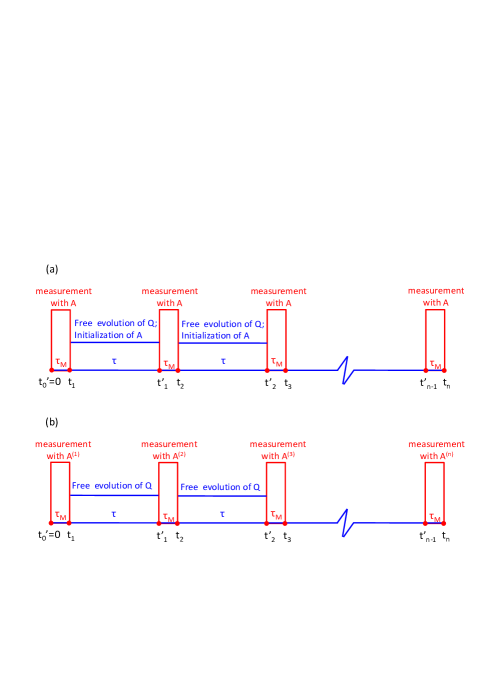
Figure 1: (color online) (a) The single-apparatus model of repeated measurements. All the measurements are performed with the same apparatus $A$. Before every measurement the state of $A$ is initialized to a given state $|\mathrm{app}\rangle$. (b) Multi-apparatus model for repeated measurements. Each measurement is done with a individual apparatus with initial state $|\mathrm{app}\rangle$.

In this paper, we discuss the quantum evolution of a dissipative TLS under repeated quantum non-demolition measurements. There are two possible models to describe the repeated quantum measurements, i.e., the single-apparatus model and the multi-apparatus model. In the single-apparatus model, all the measurements are completed via the same apparatus whose state is “initialized” to a special one in the beginning of each measurement. In the multi-apparatus model, each measurement is achieved by an individual apparatus DQAZEhalf2004 . Namely, in every measurement, only one apparatus interacts with the to-be-measured system while all the others are left alone. In the recent experimental realization of QZE in cavity QED ExpCQED , in every measurement the state of the cavity field is measured by an individual ensemble of cold atoms. It can be considered as an illustration of the multi-apparatus model.

In the current section, we prove that, regarding to the evolution of the to-be-measured system (in our case, it is the TLS together with the heat bath), the two models are equivalent. They can lead to the same evolution of the density matrix of the to-be-measured system. For the convenience of our calculation, in this paper we will use the multi-apparatus model in our discussion for QZE and QAZE from the next section.

In the following we will first show the dynamical model of a single quantum non-demolition measurement, and then do the formal calculation for the evolution of the to-be-measured system under repeated measurements with single-apparatus and multi-apparatus model. Our result shows that the density matrix of the to-be-measured system has the same time evolution in both models. For the generality of our discussion, in this section the to-be-measured system is assumed to be a general multi-level quantum system. From next section we will focus on the system of TLS together with the heat bath.

II.1 The dynamical model of a single quantum non-demolition measurement

According to the dynamical theory of quantum non-demolition measurements QM , the measurement process can be described by the coupling between the to-be-measured system $Q$ and the apparatus $A$. The total Hamiltonian of $Q$ and $A$ has an expression of conditional dynamics

$$H_{M}=\sum_{j=1}|j\rangle\langle j|\otimes H_{j}$$ (1)

where $H_{j}$ is the Hamiltonian of the apparatus $A$ with respect to the $j$-th eigenstate $|j\rangle$ of the observable of the open system. Before the measurement, the system $Q$ can be in any superposition state $\sum_{j=1}C_{j}|j\rangle$, while the apparatus is set in a pure state $|{\rm app}\rangle$. If the duration time of the measurement is $\tau_{\mathrm{M}}$, the measurement leads to the transformation

$$\sum_{j=1}C_{j}|j\rangle|\mathrm{app}\rangle\rightarrow\sum_{j=1}C_{j}|j\rangle|\mathrm{A}_{j}\rangle$$ (2)

where

$$|\mathrm{A}_{j}\rangle=e^{-iH_{j}\tau_{\mathrm{M}}}|\mathrm{app}\rangle$$ (3)

is the finial state of the apparatus with respect to the state $|j\rangle$ of the system $Q$. Therefore, in the more general case, if the initial density matrix of the system $Q$ is $\rho_{Q}$, after the measurement the density matrix of $Q$ becomes

$$\mathcal{L}\left[\rho_{Q}\right]\equiv\sum_{i,j}\langle i|\rho_{Q}|j\rangle\langle\mathrm{A}_{i}|\mathrm{A}_{j}\rangle|i\rangle\langle j|.$$ (4)

Then the effect of the quantum non-demolition measurement on the to-be-measured system $Q$ can be described by the relevant decoherence factors $\langle A_{i}|A_{j}\rangle$ in the definition (4) of the super-operator $\mathcal{L}$.

II.2 The single-apparatus model of repeated measurements

Now we consider the case of repeated measurements. As shown in Fig. 1(a) and 1(b), we assume the measurement is performed once in every time region $\left[t_{n-1}^{\prime},t_{n}\right]$ $(n=1,2,...;\ t_{0}^{\prime}=0)$ with duration $\tau_{\mathrm{M}}$. During the measurement, the Hamiltonian of the system $Q$ and the relevant apparatus is $H_{M}$. The length of the time intervals between every two neighbor measurements is assumed to be $\tau$. The system evolves freely with Hamiltonian $H_{Q}$ in the time between the measurements.

In the single-apparatus model, all the measurements are performed via the same apparatus $A$ (Fig. 1(a)). As we shown above, we assume the state of the apparatus $A$ is initialized to a given state $|{\rm app}\rangle$ before every measurement, and the information obtained by $A$ from the last measurement is “erased”. This initialization or erasing process can be done via switching on the interaction between $A$ and an external reservoir $R$, like the spontaneous emission of the two-level atom. The similar technique has also been used in our bang-bang cooling scheme for the nano-mechanical resonator NAMR .

Now we consider the evolution of the density matrix of $Q$ in the repeated-measurement process. At the initial time $t_{0}^{\prime}$, the density matrix of $Q$ and $A$ is

$$\rho_{QA}\left(t_{0}^{\prime}\right)=\rho_{Q}\left(t_{0}^{\prime}\right)|\mathrm{app}\rangle\langle\mathrm{app}|.$$ (5)

During the time region from $t_{0}^{\prime}$ to $t_{1}$, the first measurement is performed via the interaction between the system $Q$ and the apparatus $A$ while the interaction between $A$ and the reservoir $R$ is switched off. As shown above, at the ending time $t_{1}$ of the first measurement, the density matrix of the system $Q$ becomes

$$\rho_{Q}\left(t_{1}\right)=\mathcal{L}\left[\rho_{Q}\left(t^{\prime}_{0}\right)\right]$$ (6)

where the super-operator ${\mathcal{L}}$ is defined in (4).

In the time region between $t_{1}$ and $t_{1}^{\prime}$, the $Q$-$A$ interaction is switched off. The system $Q$ experiences a free evolution governed by the free Hamiltonian $H_{Q}$, while the apparatus $A$ and the reservoir $R$ experiences a coupling which induces the initialization of the state of $A$. We denote the evolution operator given by the $A$-$R$ coupling as $u_{AR}$. Then we have the total density matrix $\rho_{T}$ of $Q,$ $A$ and $R$ at time $t_{1}^{\prime}$ as

$$\rho_{T}\left(t_{1}^{\prime}\right)=u_{F}u_{AR}\rho_{T}\left(t_{1}\right)u_{AR}^{\dagger}u_{F}^{\dagger}$$ (7)

with

$$u_{F}=\exp\left[-iH_{Q}\tau\right].$$ (8)

It is pointed out that, since $u_{F}$ and $u_{AR}$ are the operators for different systems, we have

$$\left[u_{F},u_{AR}\right]=0.$$ (9)

Then we have the density matrix of the system $Q$ at time $t_{1}^{\prime}$

$$\rho_{Q}\left(t_{1}^{\prime}\right) = \mathrm{Tr}_{AR}\left[u_{F}u_{AR}\rho_{T}\left(t_{1}\right)u_{AR}^{\dagger}u_{F}^{\dagger}\right]$$ (10)

$$= u_{F}\mathrm{Tr}_{AR}\left[u_{AR}\rho_{T}\left(t_{1}\right)u_{AR}^{\dagger}\right]u_{F}^{\dagger}$$

$$= u_{F}\rho_{Q}\left(t_{1}\right)u_{F}^{\dagger}$$

$$= \mathcal{UL}\left[\rho_{Q}\left(t_{0}\right)\right]$$

with the super-operator $\mathcal{U}$ defined as $\mathcal{U}\left[...\right]=u_{F}\left[...\right]u_{F}^{\dagger}.$ On the other hand, the density matrix of the apparatus $A$ at time $t_{1}^{\prime}$ is given by

$$\rho_{A}\left(t_{1}^{\prime}\right) = \mathrm{Tr}_{QR}\left[u_{AR}u_{F}\rho_{T}\left(t_{1}\right)u_{F}^{\dagger}u_{AR}^{\dagger}\right]$$ (11)

$$= \mathrm{Tr}_{R}\left[u_{AR}\mathrm{Tr}_{Q}\left[u_{F}\rho_{T}\left(t_{1}\right)u_{F}^{\dagger}\right]u_{AR}^{\dagger}\right]$$

$$= \mathrm{Tr}_{R}\left[u_{AR}\rho_{AR}\left(t_{1}\right)u_{AR}^{\dagger}\right]$$

$$= |\mathrm{app}\rangle\langle\mathrm{app}|$$

with the density matrix $\rho_{AR}\left(t_{1}\right)$ of $A$ and $R$ at time $t_{1}:$

$$\rho_{AR}\left(t_{1}\right)=\mathrm{Tr}_{Q}\left[\rho_{T}\left(t_{1}\right)\right].$$ (12)

In the last step, we have used the fact

$$\mathrm{Tr}_{R}\left[u_{AR}\rho_{AR}\left(t_{1}\right)u_{AR}^{\dagger}\right]=|\mathrm{app}\rangle\langle\mathrm{app}|.$$ (13)

Namely, the $A$-$R$ coupling can make the density matrix of $A$ to decay to the unique steady state $|\rm{app}\rangle\langle\rm{app}|$, which is independent on the density matrix of $A$ at the time $t_{1}$ before the switching on of the $A$-$R$ coupling. That “spontaneous-emission-like process” is the physical explanation of the “initialization” of the apparatus state. Eq. (13) is applicable when the influence of the $A$-$R$ coupling on the reservoir $R$ is negligible in the total evolution from time $t_{0}^{\prime}$ to $t_{N}^{\prime}$. Then the density matrix of $Q$ and $A$ at the beginning time $t_{1}^{\prime}$ of the second measurement becomes

$$\rho_{QA}\left(t_{1}^{\prime}\right)=\rho_{Q}\left(t_{1}^{\prime}\right)|\mathrm{app}\rangle\langle\mathrm{app}|,$$ (14)

which has the same form as the one $\rho_{QA}\left(t_{0}\right)$ at the beginning of the first measurement. Therefore we can straightforwardly generalize our above discussion to the time after $t_{1}^{\prime}$. Finally we have the density matrix of the system $Q$ at the time $t_{n}^{\prime}$ after $n$ measurements and $n$ free evolutions:

$$\rho_{Q}\left(t_{n}^{\prime}\right)=\left(\mathcal{UL}\right)^{n}\left[\rho_{Q}\left(t_{0}\right)\right].$$ (15)

II.3 The multi-apparatus model of repeated measurements

Now we consider the multi-apparatus model for the repeated measurements. In this model we assume there are many individual apparatus $A^{\left(1\right)},A^{\left(2\right)},...$, each of which is in the same state $|{\rm app}\rangle$ before the measurements. In the $m$-th measurement in the time region $\left[t_{m-1}^{\prime},t_{m}\right]$, the system $Q$ only interacts with the $m$-th apparatus $A^{\left(m\right)}$, and leave the other apparatus alone. In the time interval between two measurements, the evolution of $Q$ is also governed by the same Hamiltonian $H_{Q}$. Nevertheless, the initialization of the state of the apparatus is not required in this multi-apparatus model (Fig. 1(b)).

At the beginning time $t_{0}^{\prime}$ of the first measurement, the density matrix of $Q$ and $A^{\left(1\right)}$ is

$$\rho_{QA^{\left(1\right)}}\left(t_{0}^{\prime}\right)=\rho_{Q}\left(t_{0}^{\prime}\right)|\mathrm{app}\rangle\langle\mathrm{app}|.$$ (16)

At the time $t_{1}$, after the first measurement, the density matrix of the system $Q$ is also $\mathcal{L}\left[\rho_{Q}\left(t_{0}^{\prime}\right)\right]$. At time $t_{1}^{\prime}$, the density matrix of $Q$ is

$$\rho_{Q}\left(t_{1}^{\prime}\right)=u_{F}\rho_{Q}\left(t_{1}\right)u_{F}^{\dagger}=\mathcal{UL}\left[\rho_{Q}\left(t_{0}^{\prime}\right)\right].$$ (17)

Therefore, at the beginning time $t_{1}^{\prime}$ of the second measurement, the density matrix of $Q$ and the apparatus $A^{\left(2\right)}$ is

$$\rho_{QA^{\left(2\right)}}\left(t_{1}^{\prime}\right)=\rho_{Q}\left(t_{1}\right)|\mathrm{app}\rangle\langle\mathrm{app}|$$ (18)

with the same form as $\rho_{QA^{\left(1\right)}}\left(t_{0}^{\prime}\right)$. Then at time $t_{n}^{\prime}$ after the $n$-th measurements we also have the density matrix of $Q$

$$\rho_{Q}\left(t_{n}^{\prime}\right)=\left(\mathcal{UL}\right)^{n}\left[\rho_{Q}\left(t_{0}^{\prime}\right)\right].$$ (19)

That is the same as the one (15) given by the single-apparatus model.

Therefore, the single-apparatus and multi-apparatus model for the repeated measurements can lead to the same evolution (19) of the to-be-measured system $Q$. If we only consider the evolution of the system $Q$ under the repeated measurements, we can use either single-apparatus model or multi-apparatus model in our calculation. In our discussion in the following sections, the system $Q$ includes the TLS and the heat bath which is coupled to the TLS in the time region of free evolution. We will use the multi-apparatus model to describe the repeated measurements periodically performed on the TLS.

III Repeated Measurements about Two Level System

III.1 System and measurements

In the above section we post our multi-apparatus model for the repeated quantum measurements. From this section, we show our dynamical approach for the QZE and QAZE of a dissipative TLS under repeated measurements.

We consider a TLS coupled with a heat bath which is described as a multi-mode bosonic field. The Hamiltonian of the total system is

$$H_{F} = \omega_{eg}|e\rangle^{(S)}\langle e|+\sum_{\vec{k}}\omega_{\vec{k}}a_{\vec{k}}^{{\dagger}}a_{\vec{k}}$$ (20)

$$+|e\rangle^{\left(S\right)}\langle g|\sum_{\vec{k}}\left(g_{\vec{k}}a_{\vec{k}}+g_{\vec{k}}^{\ast}a_{\vec{k}}^{\dagger}\right)+h.c.$$

Here $|g\rangle^{\left(S\right)}$ and $|e\rangle^{\left(S\right)}$ are the ground and excited states of the TLS, $a_{\vec{k}}^{{\dagger}}$ and $a_{\vec{k}}$ are respectively the creation and annihilation operators of the boson in the $\vec{k}$-th heat-bath mode with frequency $\omega_{\vec{k}}$, while $g_{\vec{k}}$ is the relevant coupling intensity between the boson and the TLS. In our Hamiltonian $H_{F}$, the rotating wave approximation is not used so that the possible effects given by the counter-rotating terms can be included Hang ; Qing .

In this paper we consider the evolution of such a dissipative TLS under repeated measurements. As shown in the above section, we use the multi-apparatus model to describe the repeated measurements. We also assume the $n$-th measurement is performed in the time region $\left[t_{n-1}^{\prime},t_{n}\right]$ $(n=1,2,...;\ t_{0}^{\prime}=0)$ with the duration time $\tau_{\mathrm{M}}$ (Fig. 2(a) and Fig. 2(b)). The time intervals between two neighbor measurements are also assumed to have the same length $\tau$. In these time intervals between the measurements, the system evolves freely under Hamiltonian $H_{F}$. In the multi-apparatus model, we assume there are many apparatuses $A^{\left(1\right)},...,A^{\left(n\right)},...$ which can be individually coupled with the TLS and distinguish between the states $|e\rangle^{\left(S\right)}$ and $|g\rangle^{\left(S\right)}$. In this paper we denote $|\rangle^{\left(S\right)}$ for the quantum state of the TLS, $|\rangle^{\left(B\right)}$ for the state of the heat bath, $|\rangle^{\left(n\right)}$ for the state of the $n$-th apparatus $A^{\left(n\right)}$ and $|\rangle^{\left(A\right)}$ for the state of all the apparatus. Before the measurement, every apparatus is  initially in a pure state. During the $n$-th measurement, the TLS is coupled with the $n$-th apparatus $A^{\left(n\right)}$ and decoupled with all the other apparatuses $A^{\left(m\neq n\right)}$.

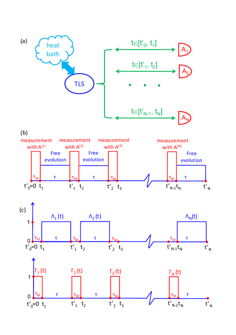
Figure 2: (color online) (a) The multi-apparatus model of the repeated quantum measurements of a dissipative TLS. In each measurement, the TLS is coupled with an individual apparatus and leaves other apparatus alone. The $n$-th measurement occurs in the time region between $t_{n-1}^{\prime}$ and $t_{n}$. The TLS is also coupled with the heat bath. (b) The time sequence of repeated measurements and free evolution governed by $H_{F}$ defined in (20). (c) The definitions of the functions $\Gamma_{n}(t)$ and $\Lambda_{n}(t)$.

As shown in Sec. II, in the quantum non-demolition measurements the coupling between the system and the apparatus $A^{\left(n\right)}$ has an expression of conditional dynamics:

$$H_{M}^{\left(n\right)}=|e\rangle^{\left(S\right)}\langle e|\otimes H_{e}^{\left(n\right)}+|g\rangle^{\left(S\right)}\langle g|\otimes H_{g}^{\left(n\right)},$$ (21)

where $H_{e}^{\left(n\right)}$ $(H_{g}^{\left(n\right)})$ is the Hamiltonian of the apparatus $A^{\left(n\right)}$ with respect to the state $|e\rangle^{\left(S\right)}$ $\left(|g\rangle^{\left(S\right)}\right)$ of the TLS. In this paper, we assume the duration time $\tau_{\mathrm{M}}$ of the measurement is so small that the interaction between the TLS and the heat bath and the decay of the excited state can be neglected during the measurement.

In the $n$-th measurement, if the state of the TLS before the measurement is $\alpha|e\rangle^{\left(S\right)}+\beta|g\rangle^{\left(S\right)}$, and the one of the apparatus $A_{n}$ is $|\mathrm{app}\rangle^{\left(n\right)}$, then the transformation given by the measurement can be described as

$$\left(\alpha|e\rangle^{\left(S\right)}+\beta|g\rangle^{\left(S\right)}\right)|\mathrm{app}\rangle^{\left(n\right)}$$

$$\rightarrow \alpha e^{-i\omega_{eg}\tau_{\mathrm{M}}}|e\rangle^{\left(S\right)}|A_{e}\rangle^{\left(n\right)}+\beta|g\rangle^{\left(S\right)}|A_{g}\rangle^{\left(n\right)}$$

with $|A_{g}\rangle^{\left(n\right)}$ and $|A_{e}\rangle^{\left(n\right)}$ the states of the apparatus attached to the ground and excited states of the TLS

$$|A_{g,e}\rangle^{\left(n\right)}=e^{-iH_{g,e}^{\left(n\right)}\tau_{\mathrm{M}}}|\mathrm{app}\rangle^{\left(n\right)}.$$ (22)

The ideality of the measurement is described by the overlap of the states $|A_{g}\rangle^{\left(n\right)}$ and $|A_{e}\rangle^{\left(n\right)}$ or the decoherence factor

$$\gamma_{n}e^{i\theta_{n}}=\ ^{\left(n\right)}\langle A_{e}|A_{g}\rangle^{\left(n\right)};\ \gamma_{n},\theta_{n}\in\mathrm{Reals}.$$ (23)

In the case of ideal projective measurement, these two states are orthogonal to each other and we have $\gamma_{n}=0$.

III.2 The total Hamiltonian in the interaction picture

Under our above assumptions, the quantum evolution of the total system including the TLS, the heat bath and the apparatuses is governed by the time-dependent Hamiltonian

$$H\left(t\right)=\omega_{eg}|e\rangle^{(S)}\langle e|+\sum_{\vec{k}}\omega_{\vec{k}}a_{\vec{k}}^{{\dagger}}a_{\vec{k}}+\sum_{n}H_{M}^{\left(n\right)}\Gamma_{n}\left(t\right)$$

$$+\left(|e\rangle^{\left(S\right)}\langle g|+|g\rangle^{\left(S\right)}\langle e|\right)\left(\sum_{\vec{k}}g_{\vec{k}}a_{\vec{k}}+h.c.\right)\sum_{n}\Lambda_{n}\left(t\right),$$

(24)

where the functions $\Gamma_{n}\left(t\right)$ and $\Lambda_{n}\left(t\right)$ are defined as in Fig. 2(c):

$$\Gamma_{n}\left(t\right)=\left\{\begin{array}[]{c}1;t\in\left[t_{n-1}^{\prime},t_{n}\right]\\ 0;\ \mathrm{otherwise}\end{array}\right.;$$ (27)

and

$$\Lambda_{n}\left(t\right)=\left\{\begin{array}[]{c}1;t\in\left[t_{n},t_{n}^{\prime}\right]\\ 0;\ \mathrm{otherwise}\end{array}\right..$$ (30)

To solve the quantum evolution of our system, we use the interaction picture where the quantum state $|\Psi\left(t\right)\rangle_{I}$ is defined as

$$|\Psi\left(t\right)\rangle_{I}=\exp\left[i\int_{0}^{t}H_{0}\left(t^{\prime}\right)dt^{\prime}\right]|\Psi\left(t\right)\rangle.$$ (31)

Here $|\Psi\left(t\right)\rangle$ is the state of the total system in the Schrödinger picture and $H_{0}$ is given by

$$H_{0}\left(t\right)=\omega_{eg}|e\rangle^{(S)}\langle e|+\sum_{\vec{k}}\omega_{\vec{k}}a_{\vec{k}}^{{\dagger}}a_{\vec{k}}+\sum_{n}H_{M}^{\left(n\right)}\Gamma_{n}\left(t\right).$$ (32)

In the interaction picture, the quantum state $|\Psi\left(t\right)\rangle_{I}$ satisfies the Schrödinger equation

$$i\frac{d}{dt}|\Psi\left(t\right)\rangle_{I}=H_{I}\left(t\right)|\Psi\left(t\right)\rangle_{I}$$ (33)

with the Hamiltonian $H_{I}\left(t\right)$ given by

$$H_{I}\left(t\right)=|e\rangle^{\left(S\right)}\langle g|\hat{f}_{B}\left(t\right)\hat{f}_{A}\left(t\right)+h.c.,$$ (34)

where the operators $\hat{f}_{B}\left(t\right)$ and $\hat{f}_{A}\left(t\right)$ are defined as

$$\hat{f}_{B}\left(t\right) = \sum_{\vec{k}}\left(g_{\vec{k}}a_{\vec{k}}e^{-i\Delta_{\vec{k}}t}+g_{\vec{k}}^{\ast}a_{\vec{k}}^{{\dagger}}e^{i\left(\omega_{eg}+\omega_{\vec{k}}\right)t}\right),$$ (35)

$$\hat{f}_{A}\left(t\right) = \sum_{n=1}\Lambda_{n}\left(t\right)M_{n}.$$ (36)

Here the detuning $\Delta_{\vec{k}}$ takes the form

$$\Delta_{\vec{k}}=\omega_{\vec{k}}-\omega_{eg}$$ (37)

and the unitary operator $M_{n}$ is given by

$$M_{n}=\prod_{l=1}^{n}\exp\left[iH_{e}^{\left(l\right)}\tau_{\mathrm{M}}\right]\exp\left[-iH_{g}^{\left(l\right)}\tau_{\mathrm{M}}\right].$$ (38)

With the help of the interaction picture, the effect of the measurements is packaged in the definition of the operator $M_{n}$. As shown below, in this interaction picture our calculations are significantly simplified and we can express all the effects from the measurements in terms of the decoherence factor $\gamma_{n}e^{i\theta_{n}}$ defined in Eq. (23). In the following two sections we will derive the short-time and long-time  evolutions of the TLS with the calculations in this interaction picture.

IV Short-time evolution: first-order perturbation theory

In this section we calculate the short-time decay rate of the excited state $|e\rangle^{\left(S\right)}$ of the TLS under repeated measurements. For simplicity, we only consider the zero-temperature case where the initial state of our system at $t=t^{\prime}_{0}=0$ as

$$|\Psi\left(0\right)\rangle_{I}=|e\rangle^{\left(S\right)}|\mathrm{vac}\rangle^{\left(B\right)}\prod_{m}|\mathrm{app}\rangle^{\left(m\right)},$$ (39)

where $|\mathrm{vac}\rangle^{\left(B\right)}$ is the vacuum state of the bosonic field and $|\mathrm{app}\rangle^{\left(m\right)}$ the initial state of the $m$-th apparatus. We consider the evolution of the system from $t=0$ to a finial time $t=t_{F}$, which, for simplicity is assumed to be an integer multiple of the period $\tau+\tau_{\mathrm{M}}$ of the measurements.

The finial state $|\Psi\left(t_{F}\right)\rangle_{I}$ of the total system is the solution of the Schrödinger equation (33). It can be expressed as a functional series of $H_{I}(t)$:

$$|\Psi\left(t_{F}\right)\rangle_{I}=\left(1-i\int_{0}^{t_{F}}H_{I}\left(t\right)dt+...\right)|\Psi\left(0\right)\rangle_{I}.$$ (40)

The survival probability $P_{e}\left(t_{F}\right)$ of the state $|e\rangle^{\left(S\right)}$ is given by

$$P_{e}\left(t_{F}\right) = 1-\ _{I}\langle\Psi\left(t_{F}\right)|(|g\rangle^{\left(S\right)}\langle g|)|\Psi\left(t_{F}\right)\rangle_{I}.$$ (41)

We can define the short-time decay rate $R(\tau,t_{F})$ of $|e\rangle^{\left(S\right)}$ as

$$P_{e}\left(t_{F}\right)=1-R(\tau,t_{F})t_{F}.$$ (42)

Therefore, $R\left(\tau,t_{F}\right)$ can also be expressed as a functional series of $H_{I}(t)$. When the total evolution time $t_{F}$ is small enough, we can only keep the lowest-order term (in our problem it is the second-order term) of $H_{I}(t)$ in $R(\tau,t_{F})$. Then we have the short-time decay rate

$$R(\tau,t_{F})\approx\frac{\tau^{2}}{t_{F}}\sum_{\vec{k}}|g_{\vec{k}}|^{2}\mathrm{sinc}^{2}\left(\Delta_{\vec{k}}\tau/2\right)$$

$$\times\left[N+2\sum_{m=1}^{N}\sum_{n=1}^{m-1}\mathrm{Re}\left(e^{i\left(n-m\right)\Delta_{\vec{k}}\left(\tau+\tau_{\mathrm{M}}\right)}{}\prod_{l=n+1}^{m}\gamma_{l}e^{i\theta_{l}}\right)\right],$$

(43)

where

$$N=\frac{t_{F}}{\tau+\tau_{\mathrm{M}}}.$$ (44)

In the case of ideal projective measurements with negligible duration time or $\tau_{\mathrm{M}}=0$, we have $\gamma_{l}=0$ and then the short-time decay rate $R(\tau,t_{F})$ in Eq. (IV) becomes a $t_{F}$-independent one:

$$R(\tau,t_{F})=R_{\mathrm{pro}}\left(\tau\right)=\tau\sum_{\vec{k}}|g_{\vec{k}}|^{2}\mathrm{sinc}^{2}\left(\Delta_{\vec{k}}\tau/2\right),$$ (45)

which is the result given by Ref. QAZ with the postulation of wave function collapse. Therefore, the QZE or QAZE based on the ideal decay rate $R_{\mathrm{pro}}\left(\tau\right)$ can also be obtained with our model.

In the case of periodic non-ideal measurements, if the common upper limit of the modului $\gamma_{n}$ of the decoherence factors in the measurements are smaller than unit, i.e., we $\gamma_{n}\leq\gamma_{\max}<1$ for any $n$, then Eq. (IV) gives

$$R(\tau,t_{F})\leq\tau\sum_{\vec{k}}|g_{\vec{k}}|^{2}\left(1+\frac{2\gamma_{\max}}{1-\gamma_{\max}}\right)\mathrm{sinc}^{2}\left(\frac{\Delta_{\vec{k}}\tau}{2}\right).$$ (46)

Therefore, for a fixed value of the total evolution time $t_{F}$, we have

$$\lim_{\tau\rightarrow 0}R(\tau,t_{F})=0.$$ (47)

It means that, in the cases of non-ideal measurements with $\gamma_{\max}<1$, the QZE also occurs in the limit that the measurement are frequent enough.

In Refs. DQAZEhalf2001 ; DQAZEhalf2001b ; DQAZEhalf2004 ; DQAZEhalf2006 , the authors have calculated the total survival probability $P_{e}\left(t_{F}\right)$ as the product of the one after each measurement, i.e., the relationship

$$P(t_{F})=P(\tau)^{N}$$ (48)

is assumed. This simplification yields that the short-time decay rate $R(\tau,t_{F})$ is the one in a single period of measurement, or

$$R(\tau,t_{F})=R(\tau,\tau).$$ (49)

In our case of $\tau\gg\tau_{\mathrm{M}}$, Eq. (49) leads to $R(\tau,t_{F})=R_{\mathrm{pro}}\left(\tau\right)$. Therefore, the intuitive treatments (48) and (49) are reasonable in the cases of ideal measurements with $\gamma_{n}=0$, and required to be improved to Eq. (43) for the cases of non-ideal measurements and non-zero $\gamma_{n}$.

IV.1 The effect given by non-ideal measurements

To further explore the physical meaning of the short-time decay rate given by Eq. (IV), we consider the simple case with identical non-ideal measurements. In this case the decoherence factor $\gamma_{n}e^{i\theta_{n}}$ takes $n$-independent value $\gamma e^{i\theta}$ ($\gamma<1$). In the large $N$ limit with $N\gg 1/(1-\gamma)$, Eq. (IV) gives a $t_{F}$-independent short-time decay rate:

$$R(\tau,t_{F}) \approx R_{\mathrm{mea}}\left(\tau\right)$$ (50)

$$\equiv \int d\eta G\left(\frac{\eta}{\tau}+\omega_{eg}\right)h\left(\gamma,\theta-\eta\right)\mathrm{sinc}^{2}\frac{\eta}{2}.\ \$$

Here we have used the approximation $\tau/(\tau+\tau_{\mathrm{M}})\approx 1$. In the above expression the spectrum function $G\left(\omega\right)$ of the heat bath defined as

$$G(\omega)=\sum_{\vec{k}}\left|g_{\vec{k}}\right|^{2}\delta(\omega-\omega_{\vec{k}})$$ (51)

and the function $h\left(\gamma,x\right)$ is given by

$$h\left(\gamma,x\right)=\frac{1-\gamma^{2}}{1+\gamma^{2}-2\gamma\cos x}.$$ (52)

It is obvious that, in the case $\gamma=0$ we have $h\left(0,x\right)=1$ and the decay rate $R_{\mathrm{mea}}\left(\tau\right)$ in Eq. (50) returns to the result $R_{\mathrm{pro}}\left(\tau\right)$ given by ideal projective measurements. In the case of repeated non-ideal measurements, the function $h\left(\gamma,\theta-\eta\right)$ in the right hand side of Eq. (50) would tune the shape of the function to be integrated and then change the value of $R_{\mathrm{mea}}\left(\tau\right)$.

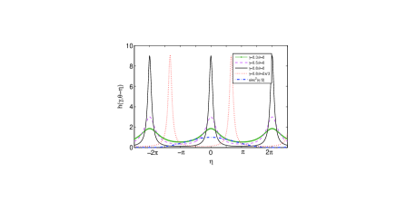
Figure 3: (color online) The function $h(\gamma,\theta-\eta)$ defined in Eq. (52). Here we plot the curves with $\gamma=0.3,\ \theta=0$ (green line with open circle); $\gamma=0.5,\ \theta=0$ (pink dashed line); $\gamma=0.8,\ \theta=0$ (black solid line) and $\gamma=0.8,\ \theta=2\pi/3$ (red dotted line). It is clearly shown that the position of the peak of $h(\gamma,\theta-\eta)$ is determined by the value of $\theta$, while the width of the peak decreases when $\gamma$ is increased. As a comparison, we also plot the function $\mathrm{{sinc}^{2}(\eta/2)}$ (blue dashed dotted line).

In Fig. 3 we plot the function $h\left(\gamma,\theta-\eta\right)$ with respect to different values of decoherence factor $\gamma e^{i\theta}$. It is easy to prove that $h\left(\gamma,\theta-\eta\right)$ takes peak value at the points $\eta=\theta+2n\pi$ ($n=0,\pm 1$,….) with the width of the order of $\arccos\gamma$. Therefore, the effects given by $h\left(\gamma,\theta-\eta\right)$ on the decay rate $R_{\mathrm{mea}}\left(\tau\right)$ in Eq. (50) seriously depend on the values of both $\gamma$ and $\theta$.

To illustrate these effects, we calculate the decay rate $R_{\mathrm{mea}}\left(\tau\right)$ of a TLS in an environment with noise spectrum

$$G(\omega)=G_{H}(\omega)\equiv\left\{\begin{array}[]{c}\frac{\omega}{\left(1+\left(\frac{\omega}{\omega_{c}}\right)^{2}\right)^{4}};\omega\geq 0\\ \ 0;\ \ \ \ \ \ \ \ \ \ \ \omega<0\end{array}\right.,$$ (55)

which is, up to a global factor, the same as the noise spectrum of the 2p-1s transition of the hydrogen atom hyd ; hyd2 . As in the case of realistic hydrogen atom, here we also take $\omega_{c}=549.5\omega_{eg}$. The decay rates $R_{\mathrm{mea}}\left(\tau\right)$ with $\theta=0,\pi/2,\pi,3\pi/2$ and various values of $\gamma$ are shown in Fig. 4.

Our results show that, with any values of $\gamma$ and $\theta$, the short-time decay rate $R_{\mathrm{mea}}\left(\tau\right)$ approaches to zero in the limit $\tau\rightarrow 0$. That is, the QZE always occurs when the measurements are repeated frequently enough. This is consistent with the conclusion in Eq. (46). On the other hand, in the limit $\tau\rightarrow\infty$, $R_{\mathrm{mea}}\left(\tau\right)$ approaches to the natural decay rate $R_{\mathrm{GR}}$ given by the Fermi golden rule:

$$R_{\mathrm{GR}}=2\pi G\left(\omega_{eg}\right).$$ (56)

Therefore, the quantum Zeno and anti-Zeno effects only occur when $\tau$ is small enough.

When the phase $\theta=0$, as shown in Fig. 4(a), both the QZE and QAZE can also appear even when the decoherence factor $\gamma$ is nonzero. However, when the value of $\gamma$ or non-ideality of the measurements is increased, the region of $\tau$ for the appearance of QZE and QAZE becomes narrower. That is, in the case of large $\tau$, the QZE and QAZE with large $\gamma$ are always less significant than the ones with small $\gamma$. In this sense the two effects are suppressed by the non-ideal measurements with real decoherence factors.

For the cases of non-zero phase $\theta$, the effects given by the non-ideal measurements are from both the non-zero value of $\gamma$ and the repeated phase modulation given by the phase factor $e^{i\theta}$. As shown in  Figs. 4(b)-4(d), the final behavior of $R_{\mathrm{mea}}$ sensitively dependents on $\theta$. Especially, with specific values of $\theta$ and $\gamma$, the non-ideal measurements can enhance either QZE or QAZE. Both the $\tau$-region where the QZE occurs and the peak value of the decay rate in the QAZE can be enlarged by the complex value of the decoherence factor $\gamma e^{i\theta}$. Finally, the total region of $\tau$ for the occurrence of QZE and QAZE with non-zero $\gamma$ is possible to be the same as the one for the cases of $\gamma=0$, or even larger than the latter. That is due to the complicated behavior of the function $h\left(\gamma,\theta-\eta\right)$.

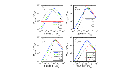
Figure 4: (color online) The short-time decay rate $R_{\mathrm{mea}}(\tau)$ defined in Eq. (50) of a dissipative TLS under repeated measurements. Here we take the noise spectrum in Eq. (55) and illustrate the cases with $\theta=0$ (a), $\theta=\pi/2$ (b), $\theta=\pi$ (c), $\theta=3\pi/2$ (d) and $\gamma=0$ (blue solid line), $\gamma=0.3$ (green dashed line), $\gamma=0.8$ (black dashed-dotted line). We also plot $R_{\mathrm{mea}}(\tau)$ (red open circle) defined in Eq. ( 57) given by frequent phase modulation pulses with approximation (59).

IV.2 The quantum Zeno and anti-Zeno effect given by phase modulation pulses

As shown in the above subsection, in the cases of non-ideal measurements with $\gamma\neq 0$, both the QZE and QAZE are possible to be enhanced in the cases with nonzero phase shift $\theta$ in each measurement. Actually in the most extreme cases of $\gamma=1$, the two effects can also appear with nonzero phase $\theta$. In that case, the measurements reduce to the phase modulation pulses which can induce periodical jumps for the relative phase between $|e\rangle^{(S)}$ and $|g\rangle^{(S)}$. The QZE and QAZE given by the phase modulation pulses have been discussed in Ref. phaseM2 ; phaseM3 in detail. Here we show that our dynamical model is also able to describe these effects.

If the pulse is repeatedly performed with period $\tau$ and negligible duration time $\tau_{\mathrm{M}}$, then the short-time decay rate in Eq. (43) becomes

$$R(\tau,t_{F}) = R_{\mathrm{PMP}}(\tau)$$ (57)

$$\equiv \int d\eta G\left(\frac{\eta}{\tau}+\omega_{eg}\right)g\left(\theta-\eta\right)\mathrm{sinc}^{2}\left(\frac{\eta}{2}\right),\ \$$

where the function $g(x)$ is defined as

$$g\left(x\right)=\frac{1}{N}\frac{\sin^{2}\left(Nx/2\right)}{\sin^{2}\left(x/2\right)}.$$ (58)

This result is essentially equivalent to the one in Refs. phaseM2 ; phaseM3 .

From now on we assume the function $G(\omega+\omega_{eg})$ has a finite width $\Delta\omega$, i.e., $G(\omega+\omega_{eg})$ takes nonzero value only in the region $-\Delta\omega<\omega<\Delta\omega$. Under this assumption, when the evolution time $t_{F}$ is large enough so that $2\pi/t_{F}$ is much smaller than the width $\Delta\omega$, we have

$$g(x)\approx 2\pi\sum_{n=-\infty}^{\infty}\delta\left(x+2n\pi\right).$$ (59)

If the period $\tau$ of the pulses is short enough so that $\tau<\pi/\Delta\omega$ and

$$G(-\pi/\tau+\omega_{eg})=G(\pi/\tau+\omega_{eg})\simeq 0,$$ (60)

the function $G(\eta/\tau+\omega_{eg})$ is localized in the region $-\pi<\eta<\pi$. Then the simplification (59) implies

$$R_{\mathrm{PMP}} \approx 2\pi G\left(\frac{\theta}{\tau}+\omega_{eg}\right)\mathrm{sinc}^{2}\left(\frac{\theta}{2}\right)$$ (61)

$$+2\pi G\left(\frac{\theta}{\tau}-\frac{2\pi}{\tau}+\omega_{eg}\right)\mathrm{sinc}^{2}\left(\frac{\theta}{2}-\pi\right),$$

where we have assumed $\theta\in\left[0,2\pi\right]$. In this case, as a result of Eq. (60), one can further find some special $\tilde{\theta}$ so that $\tilde{\theta}/\tau-2\pi/\tau<-\Delta\omega$ and $\tilde{\theta}/\tau>\Delta\omega$, which makes $G(\tilde{\theta}/\tau+\omega_{eg})\sim G(\tilde{\theta}/\tau-2\pi/\tau+\omega_{eg})\sim 0$ or $R_{\mathrm{PMP}}\sim 0$. There are also other special angles $\theta^{\ast}$ which makes $G(\theta^{\ast}/\tau+\omega_{eg})$ or $G(\theta^{\ast}/\tau-2\pi/\tau+\omega_{eg})$ take the maximum value $G^{\max}$ of $G\left(\omega\right)$. Therefore, the decay rate $R_{\mathrm{PMP}}$ can be tuned in the broad region between $0$ and some maximum value which is of the order of $2\pi G^{\max}$. This tuning effect is also predicted in Refs. phaseM2 ; phaseM3 .

We also point out that, in the limit $\gamma\rightarrow 1$ the function $h\left(\gamma,x\right)$ in the last subsection has the same behavior

$$h\left(\gamma\rightarrow 1,x\right)\approx 2\pi\sum_{n=-\infty}^{\infty}\delta\left(x+2n\pi\right)$$ (62)

as $g(x)$ in the large $N$ limit. Therefore the results in Eq. (57) for $2\pi/t_{F}<<\Delta\omega$ can also be obtained from Eq. (50).

In Fig. 4 we also plot the short-time decay rate $R_{\mathrm{PMP}}$ under approximation (59) with the spectrum (55) and different values of the angle $\theta$. It is shown that, when $\gamma$ is close to unit the short-time decay rate $R_{\mathrm{mea}}$ in Eq. (50) is quite close to $R_{\mathrm{PMP}}$. In this case the behavior of the short-time decay rate is dominated by the repeated phase modulation.

V The Long-Time Evolution: Rate Equation

In the above section we have considered the short-time evolution of the dissipative TLS under repeated measurements or phase modulation pulses. We obtain the short-time decay rates via perturbative calculation based on our pure dynamical model of repeated measurements. The perturbative approach is simple and straightforward. Nevertheless, the results are only applicable when the total evolution time $t_{F}$ is short.

In this section, we go beyond the short-time calculation and consider the long-time evolution of the TLS under repeated measurements. The problem with projective measurements has been considered in Refs. control1 ; control2 ; control3 in a semi-classical approach with measurements described by a stochastic term in the Hamiltonian. Here we provide a full-quantum theory which can be used for the cases of either ideal or non-ideal measurements. The previous results phaseM2 ; phaseM3 on the long-time evolution of a dissipative TLS under repeated phase modulation pulses can also be derived in our approach.

For simplicity, here we assume the measurements are identical with the decoherence factor $\gamma e^{i\theta}$. We first deduce the general form of the rate equation of the TLS in terms of the effective time-correlation function of the environment, and then derive the simplified form of the rate equation under the time-local and coarse-grained approximation.

V.1 The general rate equation and effective time-correlation function of the environment

To derive the rate equation for the TLS, we first consider the TLS and the apparatuses as a total system interacting with the heat bath. The evolution of the density matrix $\rho^{\left(SA\right)}$ of such a combined system can be described by master equation given by Born approximation (Eq. (9.26) of Ref. opensystem ):

$$\frac{d}{dt}\rho^{\left(SA\right)}\left(t\right)$$ (63)

$$= -\int_{0}^{t}ds\mathrm{Tr}_{B}\left[H_{I}\left(t\right),\left[H_{I}(s),\rho^{(SA)}(s)\otimes\rho^{(B)}\right]\right],\ \ \$$

where $H_{I}\left(t\right)$ is defined in Eq. (34) and $\rho^{\left(B\right)}$ is the initial density matrix of the heat bath, which is assumed to be in the thermal equilibrium state at temperature $T$. It is pointed out that, in Eq. (63) we do not perform the Markovian approximation.

The evolution equation for the density matrix $\rho^{\left(S\right)}\left(t\right)$ of the TLS can be obtained by tracing out the states of the apparatuses in Eq. (63). According to Eq. (34), in the calculation we need to evaluate the values of

$$\mathrm{Tr}_{A}\left[\hat{f}_{A}\left(t\right)\hat{f}_{A}^{{\dagger}}\left(s\right)\rho^{\left(SA\right)}\left(s\right)\right]$$ (64)

$$\mathrm{Tr}_{A}\left[\hat{f}_{A}\left(s\right)\hat{f}_{A}^{{\dagger}}\left(t\right)\rho^{\left(SA\right)}\left(s\right)\right]$$ (65)

$$\mathrm{Tr}_{A}\left[\hat{f}_{A}^{{\dagger}}\left(t\right)\hat{f}_{A}\left(s\right)\rho^{\left(SA\right)}\left(s\right)\right]$$ (66)

$$\mathrm{Tr}_{A}\left[\hat{f}_{A}^{{\dagger}}\left(s\right)\hat{f}_{A}\left(t\right)\rho^{\left(SA\right)}\left(s\right)\right]$$ (67)

with $s\leq t$. Noting that the product of $\hat{f}_{A}\left(t\right)$ ($\hat{f}_{A}^{{\dagger}}\left(t\right)$) and $\hat{f}_{A}\left(s\right)$ ($\hat{f}_{A}^{{\dagger}}\left(s\right)$) is nonzero only when there exist integers $n_{t}$ and $n_{s}$ so that $\Lambda_{n_{t}}(t)=\Lambda_{n_{s}}(s)=1$ or

$$\exists\ n_{t},n_{s},\ \mathrm{so\ that}\ t\in\left[t_{n_{t}}^{\prime},t_{n_{t}}\right];s\in\left[t_{n_{s}}^{\prime},t_{n_{s}}\right].$$ (68)

When this condition is satisfied, we separate all the apparatuses into two groups:

$$X:\{\mathrm{the\ apparatuses}\ A_{1},A_{2}...,A_{n_{s}}\}$$

$$Y:\{\mathrm{the\ apparatuses}\ A_{n_{s}+1},A_{n_{s}+2},...\}$$

Obviously, $X$ is the group of the apparatuses which interact with the system before the time $s$, while $Y$ includes the ones interact with the system after the time $s$. Therefore the density matrix $\rho^{\left(SA\right)}\left(s\right)$ can be written as

$$\rho^{\left(SA\right)}\left(s\right)=\rho^{\left(SX\right)}\left(s\right)\rho_{0}^{Y},$$ (69)

where $\rho^{\left(SX\right)}\left(s\right)$ is the reduced density matrix of the TLS together with the apparatuses in the group $X$, and $\rho_{0}^{Y}$ is given by

$$\rho_{0}^{Y}=\prod_{m=n_{s}+1}^{\infty}|\mathrm{app}\rangle^{\left(m\right)}\langle\mathrm{app}|.$$ (70)

On the other hand, Eqs. (35), (36) and (38), together with the condition $s\leq t$, yield

$$\hat{f}_{A}\left(t\right)\hat{f}_{A}^{{\dagger}}\left(s\right)=\prod_{l=n_{s}+1}^{n_{t}}\exp\left[iH_{e}^{\left(l\right)}\tau_{\mathrm{M}}\right]\exp\left[-iH_{g}^{\left(l\right)}\tau_{\mathrm{M}}\right].$$ (71)

Namely, the operator $\hat{f}_{A}\left(t\right)\hat{f}_{A}^{{\dagger}}\left(s\right)$ only operates on the state of the apparatus in the group $Y$. Then the quantity in Eq. (64) can be obtained as

$$\mathrm{Tr}_{A}\left[\hat{f}_{A}\left(t\right)\hat{f}_{A}^{{\dagger}}\left(s\right)\rho^{\left(SA\right)}\left(s\right)\right]$$ (72)

$$= \rho^{\left(S\right)}\left(s\right)\mathrm{Tr}_{A}\left[\hat{f}_{A}\left(t\right)\hat{f}_{A}^{{\dagger}}\left(s\right)\rho_{0}^{Y}\right].$$

It can be calculated easily with the simple form in Eq. (70) of $\rho_{0}^{Y}$. The terms in Eqs. (65-67) can be evaluated in the similar approach.

Then we get the rate equation

$$\frac{d}{dt}P_{e}\left(t\right)= -\int_{0}^{t}dsF_{AB}^{\left(+\right)}\left(t,s\right)P_{e}\left(s\right)$$ (73)

$$+\int_{0}^{t}dsF_{AB}^{\left(-\right)}\left(t,s\right)P_{g}\left(s\right),$$

where $P_{e}\left(t\right)=^{(S)}\!\!\langle e|\rho^{(S)}(t)|e\rangle^{\left(S\right)}$ and $P_{g}\left(t\right)=1-P_{e}\left(t\right)$ are the probabilities of the excited and ground states of the TLS. In the cases of Sec. IV where the initial state of the TLS is assumed to be $|e\rangle$, the $P_{e}\left(t\right)$ defined here becomes the survival probability defined in (41). In Eq. (73), the effective time-correlation functions $F_{AB}^{\left(\pm\right)}\left(t,s\right)$ of the environment are defined as

$$F_{AB}^{\left(\pm\right)}\left(t,s\right)=2\mathrm{Re}\left[g_{B}^{\left(\pm\right)}\left(t-s\right)g_{A}\left(t,s\right)\right],$$ (74)

where the bare correlation-functions $g_{B}^{\left(\pm\right)}$ of the heat bath are given by

$$g_{B}^{\left(+\right)}\left(t-s\right)=\mathrm{Tr}_{B}\left[\hat{f}_{B}\left(t\right)\hat{f}_{B}^{{\dagger}}\left(s\right)\rho^{\left(B\right)}\right]$$

$$= \sum_{\vec{k}}\left|g_{\vec{k}}\right|^{2}\left[\left(n_{\vec{k}}+1\right)e^{-i\Delta_{\vec{k}}\left(t-s\right)}+n_{\vec{k}}e^{i\left(\omega_{\vec{k}}+\omega_{eg}\right)\left(t-s\right)}\right],$$

$$g_{B}^{\left(-\right)}\left(t-s\right)=\mathrm{Tr}_{B}\left[\hat{f}_{B}^{{\dagger}}\left(t\right)\hat{f}_{B}\left(s\right)\rho^{\left(B\right)}\right]$$

$$= \sum_{\vec{k}}\left|g_{\vec{k}}\right|^{2}\left[n_{\vec{k}}e^{i\Delta_{\vec{k}}\left(t-s\right)}+\left(n_{\vec{k}}+1\right)e^{-i\left(\omega_{\vec{k}}+\omega_{eg}\right)\left(t-s\right)}\right]$$

with $n_{\vec{k}}=\mathrm{Tr}_{B}[a_{\vec{k}}^{{\dagger}}a_{{}_{\vec{k}}}\rho^{\left(B\right)}]$ the average number of the boson in the $\vec{k}$-th mode of the heat bath. The correlation-function of the measurements is defined as

$$g_{A}\left(t,s\right)=\mathrm{Tr}_{A}\left[\hat{f}_{A}\left(t\right)\hat{f}_{A}^{{\dagger}}\left(s\right)\rho_{0}^{Y}\right].$$ (77)

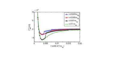
Figure 5: (color online) The effective time-correlation function $F^{(+)}_{AB}(t,0)$ defined in Eq. (74) of the environment of a dissipative TLS under repeated measurements. Here the heat bath is assumed to be at zero temperature with Ohmic spectrum (79), where $\omega_{c}=500\omega_{eg}$. The incoherence factor of the non-ideal measurements is $\gamma=0.5$ and $\theta=0$. We plot the behaviors of $F^{(+)}_{AB}$ with the measurement period $\tau=0.003/\omega_{eg}$ (blue line with open diamond), $0.005/\omega_{eg}$ (red line with open square), $0.01/\omega_{eg}$ (black line with open triangle) and $0.1/\omega_{eg}$ (green line). It is clearly shown that the long-time trail of $F^{(+)}_{AB}(t,0)$ is suppressed by the frequent measurements with small $\tau$. We also take the limit $\tau_{\mathrm{M}}=0$.

It is easy to prove that, the functions $g_{A}\left(t,s\right)$ and $g_{B}^{\left(\pm\right)}\left(t-s\right)$ decrease when the absolute value of $\left|t-s\right|$ increases. When $t$ and $s$ satisfy the condition (68) we have

$$g_{A}\left(t,s\right)=\gamma^{\left(n_{t}-n_{s}\right)}e^{i\left(n_{t}-n_{s}\right)\theta}.$$ (78)

If the condition (68) is violated we have $g_{A}\left(t,s\right)=0$.

The rate equation (73) shows that, the evolution of the probabilities $P_{e,g}\left(s\right)$ of the excited and ground states of the TLS is governed by the time-correlation functions $F_{AB}^{\left(\pm\right)}\left(t,s\right)$, which are given by both the time-correlation function of the heat bath and the decoherence factors of the measurements. The measurements tune the correlation function $F_{AB}^{\left(\pm\right)}\left(t,s\right)$ through the function $g_{A}\left(t,s\right)$. Especially, the trail of $F_{AB}^{\left(\pm\right)}\left(t,s\right)$ in the long-time-interval region with large $\left|t-s\right|$ would be suppressed by the factor $\gamma^{\left(n_{t}-n_{s}\right)}$ in the function $g_{A}\left(t,s\right)$ defined in Eq. (78).

To illustrate the effects given by the repeated measurements to the effective correlation function $F_{AB}^{\left(\pm\right)}\left(t,s\right)$, in Fig. 5 we plot $F_{AB}^{\left(+\right)}\left(t,0\right)$ for a TLS in a zero-temperature environment with Ohmic spectrum

$$G\left(\omega\right)=G_{O}\left(\omega\right)=\omega e^{-\omega/\omega_{c}}.$$ (79)

It is clearly shown that when the increasing of the frequency of the measurements, or the decreasing of the time interval $\tau$ between measurements, can lead to the suppression of the long-time trail of $F_{AB}^{\left(+\right)}\left(t,0\right)$.

One important parameter for the correlation function $F_{AB}^{\left(\pm\right)}\left(t,s\right)$ is the effective correlation time $\tau_{F}$, which gives $F_{AB}^{\left(\pm\right)}\left(t,s\right)\simeq 0$ for $\left|t-s\right|>\tau_{F}$. If $\tau_{F}$ is small enough so that the variation of the probabilities $P_{e}\left(t\right)$ and $P_{g}\left(t\right)$ is negligible in the time interval $\tau_{F}$, we can perform the time-local approximation

$$P_{e,g}\left(s\right)\approx P_{e,g}\left(t\right)$$ (80)

in Eq. (73) and significantly simplify the rate equation.

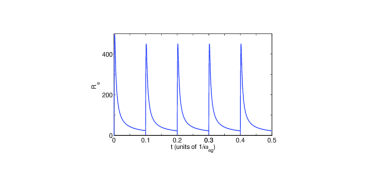
Figure 6: (color online) The decay rate $R_{e}(t)$ in Eq. (84). Here we take the measurement period $\tau=0.1/\omega_{eg}$. Other parameters are the same as the ones in Fig. 5. As proved in Eq. (87), in the long-time limit the decay rate is a periodic function of $\tau$. (Here we also take the limit $\tau_{\mathrm{M}}=0$.) The discontinuity of the function $R_{e}(t)$ at $t=n\tau\ (n=1,2,3,...)$ is due to the jumping behavior of the function $g_{A}\left(t,s\right)$ in Eq. (78).

Eq. (74) yields

$$\tau_{F}=\min\left\{\tau_{A},\tau_{B}\right\},$$ (81)

where $\tau_{A}$ and $\tau_{B}$ are the correlation times of the functions $g_{A}\left(x\right)$ and $g_{B}^{\left(\pm\right)}$. From Eq. (78) we have

$$\tau_{A}\sim\left(1-1/\ln\gamma\right)\left(\tau+\tau_{\mathrm{M}}\right).$$ (82)

In the case of ideal projective measurements we have $\tau_{A}=\tau+\tau_{\mathrm{M}}$. Therefore, Eq. (81) shows that frequent measurements with small period $\tau$ can reduce the effective correlation-time of the environment experienced by the dissipative TLS.

V.2 The master equation under time-local and coarse-grained approximation

In the following we assume the effective correlation time $\tau_{F}$ is small enough and the time-local approximation (80) can be used. Then the rate equation (73) can be simplified as

$$\frac{d}{dt}P_{e}\left(t\right)=-R_{e}\left(t\right)P_{e}\left(t\right)+R_{g}\left(t\right)P_{g}\left(t\right),$$ (83)

where the time-dependent decay rates $R_{e}\left(t\right)$ and $R_{g}\left(t\right)$ are given by

$$R_{e,g}\left(t\right)=\int_{0}^{t}dsF_{AB}^{\left(\pm\right)}\left(t,s\right).$$ (84)

On the other hand, Eq. (78) implies that

$$g_{A}\left(t,s\right)=g_{A}\left(t+\tau+\tau_{\mathrm{M}},s+\tau+\tau_{\mathrm{M}}\right).$$ (85)

This relationship, together with the definitions of $F_{AB}^{\left(\pm\right)}\left(t,s\right)$, gives

$$F_{AB}^{\left(\pm\right)}\left(t,s\right)=F_{AB}^{\left(\pm\right)}\left(t+\tau+\tau_{\mathrm{M}},s+\tau+\tau_{\mathrm{M}}\right).$$ (86)

Therefore, when $t$ is much longer than the effective correlation time $\tau_{F}$, we have

$$R_{e,g}\left(t\right) = \int_{0}^{t}dsF_{AB}^{\left(\pm\right)}\left(t,s\right)$$ (87)

$$= \int_{0}^{t}dsF_{AB}^{\left(\pm\right)}\left(t+\tau+\tau_{\mathrm{M}},s+\tau+\tau_{\mathrm{M}}\right)$$

$$= \int_{\tau+\tau_{\mathrm{M}}}^{t+\tau+\tau_{\mathrm{M}}}dsF_{AB}^{\left(\pm\right)}\left(t+\tau+\tau_{\mathrm{M}},s\right)$$

$$\approx \int_{0}^{t+\tau+\tau_{\mathrm{M}}}dsF_{AB}^{\left(\pm\right)}\left(t+\tau+\tau_{\mathrm{M}},s\right)$$

$$= R_{e,g}\left(t+\tau+\tau_{\mathrm{M}}\right),$$

and then the decay rates become periodic functions of $t$ with period $\tau+\tau_{\mathrm{M}}$, which is the same as the period of the measurements. In Fig. 6 we plot the $R_{e}\left(t\right)$ for the system in the calculation of Fig. 5. The periodic behavior of $R_{e,g}\left(t\right)$ in the large $t$ case is illustrated clearly.

If the measurements are frequent enough so that the variation of the probabilities $P_{e,g}\left(t\right)$ in the time interval $\tau+\tau_{\mathrm{M}}$ can be neglected, we can further perform the coarse-grained approximation and obtain the Markovian rate equation

$$\frac{d}{dt}P_{e}\left(t\right)=-R_{e}^{\mathrm{CG}}P_{e}\left(t\right)+R_{g}^{\mathrm{CG}}P_{g}\left(t\right)$$ (88)

with the coarse-grained decay rates

$$R_{e,g}^{\mathrm{CG}}=\lim_{N\rightarrow\infty}\frac{1}{N\left(\tau+\tau_{\mathrm{M}}\right)}\int_{0}^{N\left(\tau+\tau_{\mathrm{M}}\right)}R_{e,g}\left(t\right)dt.$$ (89)

It is easy to prove that in the zero-temperature case we have

$$R_{e}^{\mathrm{CG}} = \lim_{t_{F}\rightarrow\infty}\frac{1}{t_{F}}\int_{0}^{t_{F}}dt\int_{0}^{t}dsg_{B}^{(+)}(t-s)g_{A}(t,s)+h.c.$$ (90)

$$= \lim_{t_{F}\rightarrow\infty}\frac{1}{t_{F}}\int_{0}^{t_{F}}dt\int_{0}^{t_{F}}ds\left[g_{B}^{(+)}(t-s)g_{A}(t,s)\right]$$

$$= \lim_{t_{F}\rightarrow\infty}\frac{1}{t_{F}}\left|\int_{0}^{t_{F}}dtH_{I}(t)|\Psi(0)\rangle_{I}\right|^{2}$$

with $H_{I}(t)$ and $|\Psi(0)\rangle_{I}$ defined in Eqs. (34) and (39). Therefore $R_{e}^{\mathrm{CG}}$ at zero temperature is reduced to the short-time decay rate $R_{\mathrm{mea}}(\tau)$ being defined in Eq. (50). Namely, the decay rate given by calculation for the short-time evolution also governs the long-time evolution when the effective correlation time $\tau_{F}$ and the period of the measurements $\tau+\tau_{\mathrm{M}}$ is short enough.

Finally we discuss the behavior of the coarse-grained decay rate $R_{g}^{\rm CG}$ of the ground state. It is well-known that, for a dissipative TLS without measurements, the decay rate of the ground state is usually negligible in the zero-temperature case. However, due to the counter-rotating terms of the Hamiltonian (20), the correlation-functions $g_{B}^{\left(\pm\right)}$ defined in (V.1) and the ground-state decay rate are not absolutely zero. When the periodical measurements are performed, the value of the ground-state decay rate $R_{g}^{\rm CG}$ is also varied by the measurements, and can take significant value even in the zero-temperature.

For simplicity, we consider the simple cases with periodic identical measurements which has the decoherence factor $\gamma e^{i\theta}\ (\gamma<1)$, i.e., the cases discussed in Sec. IV A. The straightforward calculation shows that in such a case the coarse-grained decay rates are given by

$$R_{e,g}^{\rm CG}\left(\tau\right)=\int d\eta G\left(\frac{\eta}{\tau}\pm\omega_{eg}\right)h\left(\gamma,\theta-\eta\right)\mathrm{sinc}^{2}\frac{\eta}{2},$$ (91)

where “$+$” stands for $R_{e}^{\rm CG}$ and “$-$” for $R_{g}^{\rm CG}$. In the above expression, $\tau$ is length of the time interval between two measurements. The function $h$ and the spectrum $G$ of the heat bath are defined in Eq. (52) and (51).

Therefore, when there is no measurements, or in the limit $\tau\rightarrow\infty$, we have the decay rates of ground state and excited state

$$R_{e,g}^{\rm CG}(\tau\rightarrow\infty)\approx G\left(\pm\omega_{eg}\right)\int d\eta h\left(\gamma,\theta-\eta\right)\mathrm{sinc}^{2}\frac{\eta}{2}.$$ (92)

Since all the frequencies of the heat-bath are positive, we have $G\left(-\omega_{eg}\right)=0$ and then $R_{g}^{\rm CG}(\tau\rightarrow\infty)\approx 0$.

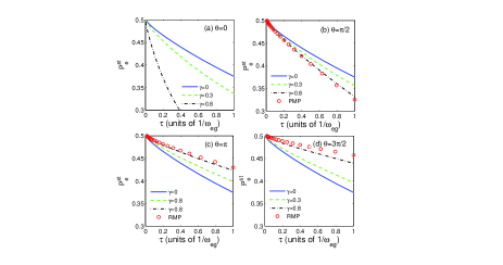
Figure 7: (color online) The probability $P_{e}^{\rm st}$ of the excited state of the TLS in the steady-state. Here we plot $P_{e}^{\rm st}$ given by Eq. (94). We take the noise spectrum in Eq. (55) and illustrate the cases with (a) $\theta=0$, (b) $\theta=\pi/2$, (c) $\theta=\pi$ and (d) $\theta=3\pi/2$, and $\gamma=0$ (blue solid line), $\gamma=0.3$ (green dashed line), $\gamma=0.8$ (black dashed-dotted line). In (b-d) we also plot the probability $P_{e}^{\rm st}$ (red open circle) given by frequent phase modulation pulses.

In the presence of periodic measurements, the decay rates $R_{e,g}^{\rm CG}$ are given by the overlap of the spectrum $G\left(\eta/\tau\pm\omega_{eg}\right)$ and the function $h\left(\gamma,\theta-\eta\right)\mathrm{sinc}^{2}(\eta/2)$, or, roughly speaking, given by the values of $G\left(\eta/\tau\pm\omega_{eg}\right)$ in the region $\eta\in[-\pi,\pi]$. We assume the function $G(x)$ takes nonzero value in the region $x\in[0,\Omega]$, then $G\left(\eta/\tau\pm\omega_{eg}\right)$ is nonzero only when $\eta\in[\mp\omega_{eg}\tau,\mp\omega_{eg}\tau+\Omega\tau]$. Therefore, when the measurements are more frequent, or the time interval $\tau$ becomes smaller, the non-zero region of $G\left(\eta/\tau-\omega_{eg}\right)$ has more and more overlaps with the region $[-\pi,\pi]$. Then the decay rates $R_{g}^{\rm CG}$ can be significant. In the limit $\tau\rightarrow 0$, both of the two functions $G\left(\eta/\tau\pm\omega_{eg}\right)$ take non-zero values only in a small region around $\eta=0$. Then we have

$$R_{g}^{\rm CG}(\tau\rightarrow 0)=R_{g}^{\rm CG}(\tau\rightarrow 0)\approx\tau h(\gamma,\theta)\int d\xi G\left(\xi\right).$$ (93)

The influence of the finite value of $R_{g}^{\rm CG}$ can be observed from the steady-state solution of the coarse-grained rate equation (88), which describes the result of the long-time evolution of the dissipative TLS under repeated measurements. According to Eq. (88), in the steady state, population probabilities $P_{g}^{\rm st}$ and $P_{e}^{\rm st}$ of the TLS in the ground and excited states can be expressed as a function of the time interval $\tau$ of the measurement:

$$P_{g}^{\rm st}(\tau)=\frac{R_{e}^{\rm CG}(\tau)}{R_{e}^{\rm CG}(\tau)+R_{g}^{\rm CG}(\tau)};\ P_{e}^{\rm st}=\frac{R_{g}^{\rm CG}(\tau)}{R_{e}^{\rm CG}(\tau)+R_{g}^{\rm CG}(\tau)}.$$

(94)

Therefore, the non-zero decay rate $R_{g}^{\rm CG}$ of the ground state leads to the non-zero population probability $P_{e}^{\rm st}$ of the excited state.

To illustrate the effects given by finite $R_{g}^{\rm CG}$, in Fig. 7(a)-7(d) we plot the population probabilities $P_{e}^{\rm st}$ with respect to different values of $\tau$ and the decoherence factor $\gamma e^{i\theta}$. As in Fig. 4, we take the noise spectrum in Eq. (55). It is clearly shown that when $\tau$ becomes small, the probability $P_{e}^{\rm st}$ becomes non-zero. In the limit $\tau\rightarrow 0$, $P_{e}^{\rm st}$ approaches $1/2$ which implies $R_{g}^{\rm CG}=R_{e}^{\rm CG}$. In Fig. 7 we also plot $P_{e}^{\rm st}$ for the cases with phase modulation pulses rather than repeated measurements. The behavior of $P_{e}^{\rm st}$ is quit similar with the one given by repeated measurements. The non-zero decay rate $R_{g}^{\rm CG}$ for the cases with phase modulation pulses is also obtained in Refs phaseM2 ; phaseM3 .

VI Conclusion and Discussion

In this paper we provide a complete dynamical model for the evolution of dissipative TLS under repeated quantum non-demolition measurements. Our model gives an explanation of QZE and QAZE without the wave function collapse postulation. The effects given by non-ideal measurements are naturally obtained in our model. The QZE and QAZE given by repeated phase modulation pulses can also be derived in our framework as a special case of non-ideal measurement.

Based on our model, we derive the short-time decay rate (43) which implies that the QZE and QAZE may be enhanced by a non-ideal measurement with complex decoherence factor. The long-time rate equation (73) is also obtained in terms of the effective time-correlation function $F_{AB}^{(\pm)}$, which describes the adjustment of the noise spectrum from the repeated measurements. The rate equation also shows that, the decay rate of the ground state of the TLS may be changed to non-zero value by the repeated measurements, and then the steady-state probabilities of the ground state and the excited state are also varied.

The effects of non-ideal measurements on QZE and QAZE obtained in our model can be observed in the experiments where the system-apparatus interactions are well controlled. Such systems are possibly to be realized by nuclear magnetic resonance or solid-state quantum devices. Although we illustrate our model with a TLS, all the techniques in this paper, including the choice of the interaction picture in Sec. II.C, the time-dependent perturbation theory in Sec. III, the master equation (63) and the separation of the apparatuses in Sec. IV.A, can be used in the cases other than TLS. Therefore our model presented in this paper can also be straightforwardly generalized to the discussions of QZE and QAZE of multi-level quantum system.

- (1) B. Misra and E. C. G. Sudarshan, J. Math. Phys. 18, 756 (1977).
- (2) A. G. Kofman and G. Kurizki, Nature 405, 546 (2000).
- (3) M. Lewenstein and K. Rzaewski, Phys. Rev. A 61, 0220105 (2000).
- (4) W. M. Itano, D. J. Heinzen, J. J. Bollinger, and D. J. Wineland, Phys. Rev. A 41, 2295 (1990).
- (5) C. Balzer, R. Huesmann, W. Neuhauser, and P. E. Toschek, Opt. Commun. 180, 115 (2000).
- (6) M. C. Fischer, B. Gutirrez-Medina, and M. G. Raizen, Phys. Rev. Lett. 87, 040402 (2001).
- (7) S. R. Wilkinson, C. F. Bharucha, M. C. Fischer, K. W. Madison, P. R. Morrow, Q. Niu, B. Sundaram, and M. G. Raizen, Nature 387, 575 (1997).
- (8) E. W. Streed, J. Mun, M. Boyd, G. K. Campbell, P. Medley, W. Ketterle, and D. E. Pritchard, Phys. Rev. Lett. 97, 260402 (2006).
- (9) B. Nagels, L. J. F. Hermans, and P. L. Chapovsky, Phys. Rev. Lett. 79, 3097 (1997).
- (10) J. Bernu, S. Delglise, C. Sayrin, S. Kuhr, I. Dotsenko, M. Brune, J. M. Raimond, and S. Haroche, Phys. Rev. Lett. 101, 180402 (2008).
- (11) A. Peres and A. Ron, Phys. Rev. A 42, 5720 (1990).
- (12) L. E. Ballentine, Found. Phys. 20, 1329 (1990).
- (13) T. Petrosky, S. Tasaki, and I. Prigogine, Phys. Lett. A 151, 109 (1990).
- (14) T. Petrosky, S. Tasaki, and I. Prigogine, Physica A 170, 306 (1991).
- (15) E. Block and P. R. Berman, Phys. Rev. A 44, 1466 (1991).
- (16) V. Frerichs and A. Schenzle, Phys. Rev. A 44, 1962 (1991).
- (17) L. E. Ballentine, Phys. Rev. A 43, 5165 (1991).
- (18) D. Homet and M. A. B. Whitaker, J. Phys. A: Math. Gen. 25, 657 (1992).
- (19) S. Pascazio, M. Namiki, G. Badurek, and H. Rauch, Phys. Lett. A 179, 155 (1993).
- (20) M. J. Gagen and G. J. Milburn, Phys. Rev. A 47, 1467 (1993).
- (21) D. Home and M. A. B. Whitaker, Phys. Lett. A 173, 327(1993).
- (22) A. L. Riveraa and S. M. Chumakov, J. Mod. Opt. 43, 839 (1994).
- (23) T. P. Altenmuller and A. Schenzle, Phys. Rev. A 49, 2016 (1994).
- (24) S. Pascazio and M. Namiki, Phys. Rev. A 50, 4582 (1994).
- (25) A. L. Rivera and S. M. Chumakov, J. Mod. Opt. 41, 839 (1994).
- (26) C. P. Sun, in Quantum Classical Correspondence: The 4th Drexel Symposium on Quantum Nonintegrability, 1994, edited by D. H. Feng and B. L. Hu (International Press, Cambridge, MA), p. 99.
- (27) C. P. Sun, X. X. Yi, and X. J. Liu, Fort. Phys. 43, 585 (1995).
- (28) A. Beige and G. C. Hegerfeldt, Phys. Rev. A 53, 53 (1996).
- (29) D. Home and M. A. B. Whitaker, Ann. Phys. 258, 237 (1997).
- (30) L. S. Schulman, Phys. Rev. A 57, 1509 (1998).
- (31) D. Z. Xu, Q. Ai, and C. P. Sun, Phys. Rev. A 83, 022107 (2011).
- (32) K. Koshino and A. Shimizu, Phys. Rep. 412, 191 (2005).
- (33) J. Ruseckas, Phys. Rev. A 66, 012105 (2002).
- (34) J. Ruseckas, Phys. Lett. A 291, 185 (2001).
- (35) J. Ruseckas and B. Kaulakys, Phys. Rev. A 63, 062103 (2001).
- (36) J. Ruseckas and B. Kaulakys, Phys. Rev. A 64, 032104 (2004).
- (37) J. Ruseckas and B. Kaulakys, Phys. Rev. A 73, 052101 (2006).
- (38) Q. Ai, D. Xu, S. Yi, A. G. Kofman, C. P. Sun, and F. Nori, arXiv: 1007.4859.
- (39) A. Peres, Am. J. Phys. 48, 931 (1980).
- (40) G. Gordon, N. Erez, and G. Kurizki, J. Phys. B: At. Mol. Opt. Phys. 40, S75 (2007).
- (41) G. Gordon, G. Bensky, D. G. Klimovsky, D. D. B. Rao, N. Erez, and G. Kurizki, New J. Phys. 11, 123025 (2009).
- (42) A. G. Kofman and G. Kurizki, Phys. Rev. Lett. 87, 270405 (2001).
- (43) G. Gordon, G. Kurizki, S. Mancini, D. Vitali, and P. Tombesi, J. Phys. B: At. Mol. Opt. Phys. 40, S61 (2007).
- (44) G. Gordon, J. Phys. B: At. Mol. Opt. Phys. 42, 223001 (2009).
- (45) V. Braginsky and F. Ya. Khalili, Quantum Measurement (Cambridge University Press, London, 1992).
- (46) P. Zhang, Y. D. Wang, and C. P. Sun, Phys. Rev. Lett. 95, 097204 (2005).
- (47) H. Zheng, S. Y. Zhu, and M. S. Zubairy, Phys. Rev. Lett. 101, 200404 (2008).
- (48) Q. Ai, Y. Li, H. Zheng, and C. P. Sun, Phys. Rev. A 81,042116 (2010).
- (49) H. E. Moses, Phys. Rev. A 8, 1710 (1973).
- (50) P. Facchi, S. Pascazio, Phys. Lett. A 241, 139 (1998).
- (51) H.-P. Breuer and F. Petruccione, The Theory of Open Quantum System (Clarendon Press, Oxford, 2006).