Fingerprints of exceptional points in the survival probability of resonances in atomic spectra

Abstract

The unique time signature of the survival probability exactly at the exceptional point parameters is studied here for the hydrogen atom in strong static magnetic and electric fields. We show that indeed the survival probability $S(t)=|\langle\psi(0)|\psi(t)\rangle|^{2}$ decays exactly as $|1-at|^{2}e^{-\Gamma_{\mathrm{EP}}t/\hbar}$ where $\Gamma_{\mathrm{EP}}$ is associated with the decay rate at the exceptional point and $a$ is a complex constant depending solely on the initial wave packet that populates exclusively the two almost degenerate states of the non-Hermitian Hamiltonian. This may open the possibility for a first experimental detection of exceptional points in a quantum system.

I Introduction

Exceptional points (EP) Kato1966 , i.e., branch point singularities in non-Hermitian physical systems, where two complex eigenvalues degenerate and the corresponding eigenstates coalesce, have shown to exhibit prominent effects not observable in their absence. Most dramatic is the influence of EPs in quantum mechanics, where effects appear which are not possible in the case of Hermitian Hamiltonians with potentials describing bound state spectra. Although the EPs are single points in an (at least) two-dimensional parameter space they influence a whole region of parameters and lead to unusual results as the permutation of eigenstates for a closed adiabatic loop in the parameter space or a special type of a geometric phase Heiss1999 . Exceptional points have recently been detected in number of physical applications. Most expamples are known for optical systems such as unstable lasers Berry2003 , waveguides Klaiman2008 and optical resonators Wiersig2008 . In quantum systems the existence of exceptional points has been proven theoretically, e.g., in atomic Latinne1995 ; Cartarius2007 or molecular Lefebvre2009 spectra, in the scattering of particles at potential barriers Hernandez2006 , in atom waves Rapedius2010 ; Cartarius2008 , and in non-Hermitian Bose-Hubbard models Graefe2008 ; Graefe2010 . The experimental verification of their physical nature was achieved in microwave cavities Dembowski2001 ; Dietz2011 . Despite this success an experimental observation in a true quantum system is still lacking. Resonances at an exceptional point exhibit, however, a unique decay behavior Heiss2010 ; Wiersig2008 ; Graefe2010 ; Longhi2010 ; Graefe2011 ; Dietz2007 and it is the purpose of this article to demonstrate that this can open the possibility for the first experimental detection of EPs in an atomic quantum system.

The most fundamental quantum objects which contain exceptional points are atoms in static external magnetic and electric fields. As such they are accessible to both experimental and theoretical methods, and thus ideally suited for studying the influence of exceptional points on quantum systems. Indeed, the existence of branch points in the resonance spectra of the hydrogen atom in crossed electric and magnetic fields was found numerically Cartarius2007 ; Cartarius2009 . Here the two field strengths play the role of two controllable parameters necessary to set the system at the exceptional points. In this article we want to demonstrate that the unique time signature of the survival probability exactly at the exceptional point parameters also appears in a detectable form in spectra of the hydrogen atom.

The article is organized as follows. In Sec. II we review how in every quantum system exhibiting exceptional points a unique time behavior of the survival probability leads to an unambiguous fingerprint of the branch point singularity. To verify the existence of this signal in a true quantum system we show that it appears for the hydrogen atom in crossed electric and magnetic fields in Sec. III. Conclusions are drawn in Sec. IV.

II Fingerprint of exceptional points in the time behavior of the survival probability

Let us first explain the motivation of our work. It has been shown theoretically in a two-dimensional model Heiss2010 , in optical microspirals Wiersig2008 , in a non-Hermitian Bose-Hubbard model Graefe2010 , and in complex crystals Longhi2010 ; Graefe2011 as well as experimentally for Rabi oscillations in a microwave cavity Dietz2007 that when the spectrum of a non-Hermitian Hamiltonian has an exceptional point then for a broad range of initial conditions the survival probability, $S(t)=|\langle\psi(0)|\psi(t)\rangle|^{2}$, decays exactly as $|1-at|^{2}e^{+2\mathrm{Im}(E_{\mathrm{EP}})t/\hbar}$, where $E_{\mathrm{EP}}$ is the complex energy of the resonance state at the EP and $a$ is a complex constant depending solely on the initial wave packet. The resonance decay rate (inverse lifetime) is defined as $\Gamma_{\mathrm{EP}}=-2\mathrm{Im}(E_{\mathrm{EP}})>0$. This behavior is in clear contrast to the purely exponential decay far away from an EP and the special condition is that the initial wave packet should populate only the exceptional eigenstate $|\psi_{\mathrm{EP}}\rangle$ and its complimentary state $|\chi\rangle$ as obtained from the Jordan chain formalism such that $|\psi_{\mathrm{EP}}\rangle\langle\chi|+|\chi\rangle\langle\psi_{\mathrm{EP}}|=\hat{1}$ (see a detailed explanation in Sec. 9.2 of Ref. Moiseyev2011 where the closure relations for non-Hermitian Hamiltonian with an incomplete spectrum is discussed in detail). In this article we will demonstrate this behavior of the survival probability for a quantum mechanical system.

Let us give here a simple explanation for this unusual situation. The EP is associated with a situation where $\hat{H}(\lambda)|\psi_{j}\rangle=E_{j}|\psi_{j}\rangle$ such that for $\lambda\to\lambda_{\mathrm{EP}}$ two eigenvalues degenerate, $E_{j}-E_{j^{\prime}}\to 0$ (i.e., upon coalescence $E_{j}=E_{j^{\prime}}\equiv E_{\mathrm{EP}}$) and also the corresponding eigenstates coalesce $\psi_{j}\to\psi_{j^{\prime}}$ (up to a phase factor $i$ Moiseyev2011 , i.e., upon coalescence $\psi_{j}=i\psi_{j^{\prime}}\equiv\psi_{\mathrm{EP}}$) such that

$${\hat{M}}|\psi_{\mathrm{EP}}\rangle=0$$ (1)

where

$${\hat{M}}=\hat{H}-E_{\mathrm{EP}}$$ (2)

and $\Gamma_{\mathrm{EP}}=-2\mathrm{Im}(E_{\mathrm{EP}})$ is the decay rate of the system.

Let us take as a basis set consisting of $\psi_{\mathrm{EP}}$ and its complimentary state $\chi$ for the initial wave packet. In this basis the $2\times 2$ matrix representation of $\hat{M}$ is a matrix $\bm{M}$ for which $\bm{M}^{2}=0$. Therefore

$$\bm{U}(t\leftarrow 0) =e^{-i\bm{H}t/\hbar}=e^{-iE_{\mathrm{EP}}t/\hbar}e^{-i\bm{M}t/\hbar}$$

$$=e^{-iE_{\mathrm{EP}}t/\hbar}\sum_{n}\frac{(-i\bm{M}t/\hbar)^{n}}{n!}$$

$$=e^{-iE_{\mathrm{EP}}t/\hbar}(\bm{I}_{2\times 2}-i\bm{M}t/\hbar)\,.$$ (3)

Consequently for any initial state $\psi(t=0)$ which is a linear combination of $\psi_{\mathrm{EP}}$ and its complimentary state $\chi$ then

$$\langle\psi(t=0)|\bm{U}(t\leftarrow 0)|\psi(t=0)\rangle\\ =e^{-iE_{\mathrm{EP}}t/\hbar}(1-it\langle\psi(t=0)|\bm{M}|\psi(t=0)\rangle/\hbar)$$ (4)

and for real values of $\langle\psi(t=0)|\bm{M}|\psi(t=0)\rangle$ the survival probability is given by

$$S(t)=|\langle\psi(t=0)|\bm{U}(t\leftarrow 0)|\psi(t=0)\rangle|^{2}\\ =\left(1+[\langle\psi(t=0)|\bm{M}|\psi(t=0)\rangle/\hbar]^{2}t^{2}\right)e^{+2\mathrm{Im}(E_{\mathrm{EP}})t/\hbar}.$$ (5)

For complex values of $\langle\psi(t=0)|\bm{M}|\psi(t=0)\rangle$ an additional term linear in $t$ is added. Surly, the quadratic dependence for short times is not surprising. What is important here is that there are no terms of order higher than $t^{2}$ so that the time dependence remains $t^{2}$ for all times. This provides a unique fingerprint proving unambiguously the presence of an exceptional point since the power series expansion of Eq. (3) stopping after the linear term requires the presence of an EP. The effect even remains in a larger vicinity around the branch point singularity. Observations which are similar to exceptional points but not connected to true branch points as narrow avoided crossings for Wannier-Stark resonances Glueck2002 are not sufficient.

III Non-exponential decay of resonances in spectra of the hydrogen atom

In our study the resonances are calculated numerically exact by the diagonalization of a matrix representation of the Hamiltonian. Without relativistic corrections and finite nuclear mass effects Schmelcher1993 the Hamiltonian reads in atomic units

$$H=\frac{1}{2}\bm{p}^{2}-\frac{1}{r}+\frac{1}{2}\gamma L_{z}+\frac{1}{8}\gamma^{2}(x^{2}+y^{2})+fx,$$ (6)

where $L_{z}$ is the $z$ component of the angular momentum. The strengths of the electric and magnetic fields are labeled $f$ and $\gamma$, respectively. We exploit the fact that the parity with respect to the $(z=0)$-plane is a constant of motion and include in all our calculations only resonances with even $z$-parity.

To uncover the decaying unbound resonance states we use the complex rotation method Reinhardt1982 ; Moiseyev1998 ; Moiseyev2011 , for which the coordinates of the system $\bm{r}$ are replaced with the complex rotated ones $\bm{r}e^{\mathrm{i}\vartheta}$. For the application of the complex rotation method to hydrogen spectra see Delande1991 . This procedure renders the resonance wave functions square integrable so that that they are automatically included in the spectrum as new discrete eigenstates with complex eigenvalues in the matrix representation. The real parts of the complex energies represent their energies and the imaginary parts their widths (lifetimes). After introducing complex dilated semiparabolic coordinates Main1994 the Schrödinger equation of the Hamiltonian (6) assumes in a basis representation the form of a generalized eigenvalue problem

$$\bm{A}(\gamma,f)\Psi=2|b|^{4}E\bm{B}\Psi$$ (7)

with a complex symmetric matrix $\bm{A}(\gamma,f)$ and a real symmetric matrix $\bm{B}$. In this equation $b$ is the complex dilation parameter and $E$ the complex resonance energy. The eigenstates can be normalized such that $\left(\Psi_{i}|\bm{B}|\Psi_{j}\right)=\delta_{ij}$, where the round braces indicate an inner product in which complex parts originating exclusively from the complex dilation parameter $b$ are not conjugated, which is the appropriate inner product for complex scaled wave functions (c-product, cf. Refs. Moiseyev1998 ; Moiseyev2011 ). Note that this normalization does not hold at an exceptional point where each of the two states is orthogonal to itself Moiseyev2011 .

We first demonstrate that the decay signal of the probability density according to Eq. (4),

$$S_{\mathrm{m}}(t)=\exp\left[2\mathrm{Im}(E_{\mathrm{EP}})t\right]\left|1-i(\Psi_{0}|\bm{M}|\Psi_{0})t\right|^{2},$$ (8a)

can be found in the quantum spectrum of the hydrogen atom in a large region around the exceptional point, where in our case the matrix $$\bm{M}$$ of Eq. (2) is given by

$$\bm{M}=\bm{A}(\gamma,f)/(2|b|^{4})-E_{\mathrm{EP}}\bm{B}.$$ (8b)

The subscript $\mathrm{m}$ of $S_{\mathrm{m}}$ in Eq. (8a) is given in order to emphasize the fact that the survival probability is calculated here using the matrix representation of the Hamiltonian given by Eq. (8b). This is to distinguish from the direct evaluation of the survival probability as discussed later [Eq. (13)]. For this purpose we calculate resonance spectra for several small distances $\delta$ to the exceptional point at $(f_{\mathrm{EP}},\gamma_{\mathrm{EP}})$ in the space of the two field strengths, i.e., we use

$$f=f_{\mathrm{EP}}(1-\delta),\quad\gamma=\gamma_{\mathrm{EP}}(1-\delta).$$ (9)

For small $\delta$ the two eigenstates $\Psi_{1}$ and $\Psi_{2}$ belonging to the branch point singularity can be identified clearly. Note, however, that due to roundoff errors in the numerical calculations $\delta$ never ever gets strictly the value $0$ and always $\delta\neq 0$. As we will show in this article even when $\delta\neq 0$, i.e., when we have two almost degenerate states and the spectrum is complete the fingerprint of the EPs (strictly obtained only exactly at the coalescence of two eigenstates) on the survival probability is still pronounced.

It is well known for exceptional points that $\Psi_{1}$ and $\Psi_{2}$ converge to the single independent eigenstate with the phase relation

$$\Psi_{\mathrm{EP}}=\Psi_{1}=i\Psi_{2}$$ (10)

for $\delta\to 0$ Moiseyev2011 . A complete basis in the corresponding two-dimensional subspace is spanned by $\Psi_{\mathrm{EP}}$ and the associated vector $\Psi_{\mathrm{a}}$,

$$(\bm{A}(\gamma,f)-2|b|^{4}E_{\mathrm{EP}}\bm{B})\Psi_{\mathrm{a}}=\Psi_{\mathrm{EP}},$$ (11)

where $\Psi_{\mathrm{a}}$ is essential for a decay signal of the form (8a) Heiss2010 . Despite the convergence of $\Psi_{1}$ and $\Psi_{2}$ to the same state it is possible to extract an adequate superposition of $\Psi_{\mathrm{EP}}$ and $\Psi_{\mathrm{a}}$, viz.

$$\Psi_{0}=\sqrt{(1+1/\sqrt{\delta})/2}\,\Psi_{1}+\sqrt{(1-1/\sqrt{\delta})/2}\Psi_{2}.$$ (12)

As we get closer to the EP when $\delta\to 0$ the amplitudes of $\Psi_{1}$ and $\Psi_{2}$ approach infinitely large values. However, the initial wave packet $\Psi_{0}$ remains c-normalized. About the complex normalization rather than using the conventional scalar product for calculating the norm of a vector state read Ref. Moiseyev2011 .

We choose the exceptional point labeled 8 in Table I of Ref. Cartarius2009 at the field strengths $f=0.0002177$ and $\gamma=0.004604$, and with the complex energy $E_{\mathrm{EP}}=-0.022135-0.00006878i$ (all values in atomic units). The survival probability for the superposition (12) is plotted in Fig. 1

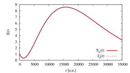
Figure 1: (Color online) Survival probability for the resonances at the exceptional point labeled 8 in Ref. Cartarius2009 with an offset of $\delta=10^{-5}$. Shown are the direct evaluation $S_{\mathrm{d}}(t)$ according to Eq. (13) and the expected form $S_{\mathrm{m}}(t)$ of Eq. (8a) including a linear term in $t$ besides the exponential decay. Note that on the scale of the figure the survival probabilities calculated by both methods are not distinguishable. Since we use here the c-product rather than the regular scalar product the survival probability can assume values larger than one. This non-physical behavior results from the way we normalize $\Psi_{0}$ [see Eq. (12)]. As we will show later this problem disappears when the initial wave packet is prepared by using a laser excitation of the field-free ground state. On the c-product read in Refs. Moiseyev1998 ; Moiseyev2011 .

for an offset $\delta=10^{-5}$. At an exceptional point we expect a decay of the survival probability in the form (8a). The corresponding numerical result is shown with the solid red line in Fig. 1, where we found $(\Psi_{0}|M|\Psi_{0})=(3.83-4.58i)\times 10^{-4}$. Since we use here the c-product Moiseyev1998 ; Moiseyev2011 rather than the regular scalar product the survival probability can assume values larger than one for the mathematical choice given in Eq. (12). Additionally, we calculate the survival probability directly without any assumption about its shape close to an exceptional point, i.e., we evaluate

$$S_{\mathrm{d}}(t)=\left|\sum_{i}(\Psi_{0}|\bm{B}|\Psi_{i})(\Psi_{i}|\bm{B}|\Psi_{0})\exp\left(-iE_{i}t\right)\right|^{2},$$ (13)

where we use 100 eigenvectors of the matrix diagonalization in the energy vicinity of the EP for the basis states $\Psi_{i}$. The blue dashed line in Fig. 1 shows the results of the latter method. As can be seen clearly both methods agree very well, which proves that the description of the decay with the linear term in (8a) is correct.

Obviously the polynomial contribution influences the decay significantly, i.e., the unique time behavior of the resonances at an exceptional point is a relevant effect in matter waves and can unambiguously be found for atomic resonances.

The typical time signal of an exceptional point is even present at larger distances $\delta$. In Fig. 2(a)

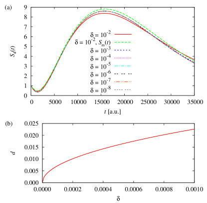
Figure 2: (Color online) (a) Survival probability $S_{\mathrm{d}}(t)$ for the same exceptional point as in Fig. 1 but for several different offsets $\delta=10^{-8}\dots 10^{-2}$. Small deviations only appear for the largest $\delta=10^{-2}$. In this case also a small difference to the shape $S_{\mathrm{m}}(t)$ at an exceptional point becomes observable. (b) The modulus $d=\left<\Psi_{1}+i\Psi_{2}\middle|\Psi_{1}+i\Psi_{2}\right>$ vanishes at the exceptional point as is expected due to the phase relation (10).

we plot the direct evaluation (13) for the same exceptional point as in Fig. 1 but for several different offsets $\delta=10^{-8}\dots 10^{-2}$. For all of these distances the two vectors belonging to the branch point are well defined. Almost all calculations provide exactly the same results. Only for $\delta=10^{-2}$ we observe a slight difference to the other calculations. At this distance also the validity of the matrix representation (8a) including only the two components associated with the exceptional point breaks down, however, the differences are still small. The corresponding line $S_{\mathrm{m}}(t)$ is included in the figure. For all other values of $\delta$ shown we checked that the results of both methods agree completely, which demonstrates that the structure of Eq. (3), which is only fulfilled in the presence of an exceptional point, survives in a larger vicinity around the branch point. The signal keeps its unique structure. To verify that we obtain the correct vectors $\Psi_{1}$ and $\Psi_{2}$ in all calculations we plot the modulus $d=\left<\Psi_{1}+i\Psi_{2}\middle|\Psi_{1}+i\Psi_{2}\right>$ in Fig. 2(b). According to the phase relation (10) $d$ must vanish in the limit $\delta\to 0$. Exactly this behavior is found.

So far we demonstrated that it is possible to find an adequate superposition of the two eigenvectors, however, we want to show furthermore that this signal can be excited in a realistic case. Is it possible to occupy such a superposition in an experimental situation? To investigate this question we assume a hydrogen atom in external fields, where the electron is in the orbital $2p$, $m=0$, for which any perturbation due to the fields we use can be ignored. The eigenstates at the exceptional point are excited with a laser polarized linearly along the direction of the static magnetic field. We use a Gaussian pulse shape of the form

$$E(\omega)\sim\exp\left(-\sigma(\omega-\omega_{0})^{2}\right),\quad\omega_{0}=\mathrm{Re}(E_{\mathrm{bp}})-E_{\mathrm{I}},$$ (14)

where $E_{\mathrm{I}}$ is the energy at the initial state $\Psi_{\mathrm{I}}$ ($2p$, $m=0$). The width was chosen to be $\sigma=1000/\omega_{0}$. Then the occupation amplitude for a transition to eigenstate $\Psi_{i}$ of the Hamiltonian is

$$A_{i}=\int d\omega E(\omega)\frac{\left(\Psi_{\mathrm{I}}\middle|D\middle|\Psi_{i}\right)}{E_{2p_{z}}-E_{\mathrm{bp}}+\hbar\omega}$$ (15)

with the dipole operator $D$ for the present choice of the light pulse.

Fig. 3(a)

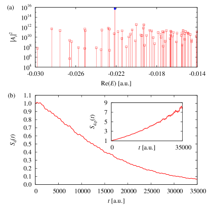
Figure 3: (Color online) (a) Occupation probabilities $|A_{i}|^{2}$ in arbitrary units for resonances in an energy vicinity of the exceptional point. The two resonances connected with the exceptional point are marked with blue (filled) circles. On the scale of our plot the two almost degenerate states are not distinguishable. (b) Survival probability for the excited state $\Psi_{\mathrm{F}}$, which is prepared by using a laser to excite the field-free ground state [see Eq. (16)]. The division by the exponential part in the inset demonstrates the presence of the polynomial contribution. The behavior of the survival probability as presented here is exactly as the analytical expression given in Eq. (8a).

shows the occupation probability $|A_{i}|^{2}$ versus real part of the energy for the states in the vicinity of the branch point. One can see that the two states connected with the branch point (marked with filled blue circles) have an occupation probability almost three orders of magnitude larger than all other states. This does not tell us, however, whether or not an adequate superposition of the two dominating states similar to the mathematical case in Eq. (12) can be achieved. Thus, we construct the normalized state

$$\Psi_{\mathrm{F}}=\frac{\tilde{\Psi}_{\mathrm{F}}}{\sqrt{(\tilde{\Psi}_{\mathrm{F}}|\bm{B}|\tilde{\Psi}_{\mathrm{F}})}},\quad\tilde{\Psi}_{\mathrm{F}}=\sum_{i}A_{i}\Psi_{i}$$ (16)

occupied by the laser with the states shown in Fig. 3(a). The survival probability is calculated according to Eq. (13) with $\Psi_{\mathrm{F}}$ instead of $\Psi_{0}$. Fig. 3(b) shows the results. The small oscillations are due to the weaker excitations of the neighboring states. They disappear for a pulse denser in frequency space. The dominating signal is still formed by the two states associated with the exceptional point. The linear part in the time behavior (8a) is weaker than in the mathematical case $\Psi_{0}$ of Eq. (12), however, it is present and is expressed in the non-exponential decay. After the division by the exponential part the polynomial contribution of the physical (observable) survival probability calculated for the initial wave packet $\Psi_{\mathrm{F}}$ [see Eq. (16)] is given by

$$S_{\mathrm{d,p}}(t)=S_{\mathrm{d}}(t)/\exp\left(2\mathrm{Im}(E_{\mathrm{EP}})t\right).$$ (17)

To demonstrate that the origin of this signal is in fact the structure (8a) originating from an exceptional point we calculated the matrix element $(\Psi_{\mathrm{F}}|M|\Psi_{\mathrm{F}})=(0.226+5.25i)\times 10^{-5}$. The line $\left|1-i(\Psi_{0}|M|\Psi_{0})t\right|^{2}$ is not distinguishable from the full numerical result presented in Fig. 3(b).

IV Conclusion

We proved in this article that any quantum system exhibiting exceptional points shows a time evolution of the form (3) for two resonances exactly at the EP, i.e., the decay includes a quadratic term as in Eq. (5) which is distinct from the typical exponential decay apart from branch point singularities. Here it is important to note that this effect is not only observable exactly at the parameters of the EP but can rather be seen in a large vicinity. In our study we found it still for a relative offset of the parameters of $\delta=10^{-2}$.

We were furthermore able to demonstrate that it is possible to excite an adequate superposition of the eigenvector at an exceptional point and its associate counterpart in a realistic physical situation such that the unique time signal becomes observable in atomic spectra. The quadratic term significantly influences the survival probability we found for the hydrogen atom in crossed electric and magnetic fields. It is an effect that leaves clear signatures in the decay of resonances in quantum systems and obviously opens a new possibility to detect an unambiguous fingerprint of an exceptional point accessible with experimental methods. It might such facilitate the first experimental detection of exceptional points in a true quantum system.

In this article the time evolution of the resonances excited with the laser pulse (14) is evaluated with the survival probability calculated from the spectrum via the c-product Moiseyev2011 ; Moiseyev1978 . Both its modulus and phase have experimental consequences Barkay2001 . In the realistic physical situation shown in Fig. 3 the survival probability describes the decay of a resonance state in time. Thus one has to measure the decaying occupation of such a state. This can presumably be detected with a second laser as already indicated Heiss2010 . Furthermore, an extraction of the time signal from the spectrum is possible and has already been used for microwave cavities Dietz2007 via a Fourier transform. In this context we should mention that the ultra-strong magnetic and electric fields we have used in our calculations are due to our computational limitations to exceptional points associated with low-lying resonance positions. However, the phenomenon discussed here appears for highly excited resonances as well. In such cases much weaker and feasible external fields are required to observe the unique survival probability of a wave packet, which initially populates mainly the two almost degenerate states associated with the exceptional point.

- (1) T. Kato, Perturbation theory for linear operators (Springer, Berlin, 1966)
- (2) W. D. Heiss, Eur. Phys. J. D 7, 1 (1999)
- (3) M. V. Berry, J. Mod. Optics 50, 63 (2003)
- (4) S. Klaiman, U. Günther, and N. Moiseyev, Phys. Rev. Lett. 101, 080402 (2008)
- (5) J. Wiersig, S. W. Kim, and M. Hentschel, Phys. Rev. A 78, 053809 (2008)
- (6) O. Latinne, N. J. Kylstra, M. Dörr, J. Purvis, M. Terao-Dunseath, C. J. Joachain, P. G. Burke, and C. J. Noble, Phys. Rev. Lett. 74, 46 (1995)
- (7) H. Cartarius, J. Main, and G. Wunner, Phys. Rev. Lett. 99, 173003 (2007)
- (8) R. Lefebvre, O. Atabek, M. Šindelka, and N. Moiseyev, Phys. Rev. Lett. 103, 123003 (2009)
- (9) E. Hernández, A. Jáuregui, and A. Mondragán, Journal of Physics A: Mathematical and General 39, 10087 (2006)
- (10) K. Rapedius, C. Elsen, D. Witthaut, S. Wimberger, and H. J. Korsch, Phys. Rev. A 82, 063601 (Dec 2010)
- (11) H. Cartarius, J. Main, and G. Wunner, Phys. Rev. A 77, 013618 (2008)
- (12) E. M. Graefe, U. Günther, H. J. Korsch, and A. E. Niederle, J. Phys. A 41, 255206 (2008)
- (13) E.-M. Graefe, H. J. Korsch, and A. E. Niederle, Phys. Rev. A 82, 013629 (2010)
- (14) C. Dembowski, H.-D. Gräf, H. L. Harney, A. Heine, W. D. Heiss, H. Rehfeld, and A. Richter, Phys. Rev. Lett. 86, 787 (2001)
- (15) B. Dietz, H. L. Harney, O. N. Kirillov, M. Miski-Oglu, A. Richter, and F. Schäfer, Phys. Rev. Lett. 106, 150403 (2011)
- (16) W. D. Heiss, Eur. Phys. J. D 60, 257 (2010)
- (17) S. Longhi, Phys. Rev. A 81, 022102 (2010)
- (18) E.-M. Graefe and H. F. Jones, “PT-symmetric sinusoidal optical lattices at the symmetry-breaking threshold,” (2011), arXiv:1104.2838
- (19) B. Dietz, T. Friedrich, J. Metz, M. Miski-Oglu, A. Richter, F. Schäfer, and C. A. Stafford, Phys. Rev. E 75, 027201 (2007)
- (20) H. Cartarius, J. Main, and G. Wunner, Phys. Rev. A 79, 053408 (2009)
- (21) N. Moiseyev, Non-Hermitian Quantum Mechanics (Cambridge University Press, Cambridge, 2011)
- (22) M. Glück, A. R. Kolovsky, and H. J. Korsch, Phys. Rep. 366, 103 (2002)
- (23) P. Schmelcher and L. S. Cederbaum, Chem. Phys. Lett. 208, 548 (1993)
- (24) W. P. Reinhardt, Ann. Rev. Phys. Chem. 33, 223 (1982)
- (25) N. Moiseyev, Phys. Rep. 302, 212 (1998)
- (26) D. Delande, A. Bommier, and J. C. Gay, Phys. Rev. Lett. 66, 141 (1991)
- (27) J. Main and G. Wunner, J. Phys. B 27, 2835 (1994)
- (28) N. Moiseyev, P. R. Certain, and F. Weinhold, Mol. Phys. 36, 1613 (1978)
- (29) H. Barkay and N. Moiseyev, Phys. Rev. A 64, 044702 (Sep 2001)