Perturbations in dark energy models with evolving speed of sound

Abstract

The behavior of perturbation in scalar field dark energy and its consequent effect on the cold dark matter (CDM) power spectrum is well understood to be governed by the equation of state (EOS) parameter and the effective speed of sound (ESS) of dark energy. In this paper, we investigate whether dark energy models whose ESS are epoch dependent leaves any distinct imprints on the large scale CDM power spectrum. In particular, we compare the cases where the ESS is decreasing with time with those where it increases. The CDM power spectrum is found to be generically suppressed in these cases as compared to the $\Lambda$CDM model. The degree of suppression at different length scales can, in principle, reflect the evolving nature of the ESS of dark energy. However, we find that the effect on the CDM power spectrum in cases where the ESS of dark energy is evolving with constant EOS parameter is significantly smaller as compared to the situation where ESS is constant whereas EOS parameter is evolving. Further, it is also shown that the effect of different evolution of ESS for a given evolution of EOS parameter of dark energy on the CDM power spectrum is significant only at the intermediate scales (around $k\sim 0.01h/Mpc$). At scales much smaller and larger than the Hubble radius, it is the evolution of EOS parameter of dark energy which governs the degree of suppression of CDM power spectrum with respect to the $\Lambda$CDM model.

I Introduction

It is now evident from numerous cosmological observations that our Universe is undergoing accelerated expansion at the present epoch Reiss-1998 ; Perlmutter-1998 ; Spergel-2007 ; Komatsu-2008 ; Komatsu-2010 . This profound discovery triggered a flood of investigations both at the theoretical and experimental front to understand the reason for this accelerated expansion. The theoretical explanation for this observed late time accelerated expansion can broadly be classified into two categories. The first explanation is based on the assumption that gravity as described by the Einstein’s general theory of relativity (GTR) is valid on the cosmological scale. This assumption then forces us to invoke some exotic matter known as dark energy to drive the late time accelerated expansion of the universe. If not the dark energy, then the only other way of explaining this accelerated expansion is to modify the theory of gravity from the standard GTR. In the present work we shall only consider the first case, viz., the one where the accelerated expansion is driven by dark energy.

Numerous models of dark energy have been investigated in the literature, these include quintessence, tachyon, k-essence, Chaplygin, gas etc. (for details, see Refs.Paddy-2003 ; Sahni-2004 ; Copeland-2006 ; Sahni-2006 and the references therein). It is now a big challenge to observationally test the predictions of these models. One of the ways of distinguishing various models of dark energy is to investigate how cold dark matter (CDM) clusters on cosmological scales. In this paper we shall investigate how a general class of scalar field models of dark energy influences the large scale CDM power spectrum.

It is well known that scalar field models of dark energy can lead to degenerate evolution of the scale factor Paddy-2002 ; Feinstein-2002 . Therefore, the evolution of scale factor is insufficient to distinguish scalar field models of dark energy. Hence, it is also necessary to take into account the consequence of perturbation in dark energy on cosmological observable such as CDM matter power spectrum. Although, the evolution of scale factor and the growth of CDM perturbations does not uniquely characterize the nature of scalar field lagrangian of the dark energy (see Ref.Sanil-2008b for details), however, such studies can be useful in at least ruling out some of the models.

Evolution of perturbations in dark energy and how it influences CDM power spectrum and the integrated Sachs-Wolfe (ISW) effect in the cosmic microwave background (CMB) have been investigated in the literature Hu-2001 ; Erickson-2002 ; Weller-2003 ; DeDeo-2003 ; Bean-2004 ; Gordon-2004 ; Gordon-2005 ; Corasaniti-2005 ; Hannestad-2005 ; Abramo-2007 ; Sanil-2008a ; Ballesteros-2008 ; Gorini-2008 ; Park-2009 ; Dent-2009 ; Abramo-2009 ; Jassal-2009 ; Sapone-2009 ; Sergijenko-2009 ; Jassal-2010 ; Putter-2010 ; Sanchez-2010 ; Ballesteros-2010 ; Karwan-2011 . It is well understood from these studies that CDM power spectrum is suppressed in a generic scalar field model of dark energy as compared to the same in $\Lambda$CDM model. The degree of suppression depends on how scale factor as well as perturbations in dark energy evolves. It is important to take into account the role played by the perturbations in dark energy for the system of equations to be consistent with Eistein’s equation Sanil-2008a ; Park-2009 .

In general, any minimally coupled scalar field model of dark energy can be characterized by the behavior of the following two parameter: (1) equation of state (EOS) $w$, and (2) the effective speed of sound (ESS) $c_{e}$. Most studies on the influence of perturbation in dark energy involves the case where $c_{e}$ and $w$ are constants (see for instance, Refs.Sapone-2009 ; Ballesteros-2010 ). Perturbations in dark energy models where ESS parameter $c_{e}$ is epoch dependent have also been investigated DeDeo-2003 ; Putter-2010 . However, the evolution of $c_{e}$ was fixed by the specific model of dark energy under investigation. Our aim in this paper is to parameterize the evolution of $c_{e}$ as a function of scale factor and to study how perturbations in such dark energy models influences the CDM power spectrum.

In this paper, we shall consider a class of k-essence dark energy models with lagrangian of the form $\mathcal{L}(X,\phi)=F(X)-V(\phi)$, where $X=(1/2)\partial_{\mu}\phi\partial^{\mu}\phi$ is the kinetic term. We shall first present a method of reconstructing the form of $F(X)$ and $V(\phi)$ from a given evolution of EOS parameter $w(a)$ and ESS parameter $c_{e}(a)$ with scale factor. Using this method, we shall reconstruct few models of dark energy starting from a desired evolution of $w(a)$ and $c_{e}(a)$. The evolution of perturbation in dark energy is investigated for the following cases (i) constant $w$ and $c_{e}$, (ii) either of $w$ and $c_{e}$ is evolving, and (iii) both $w$ and $c_{e}$ evolving. The growth of large scale CDM perturbation is compared in these models. It is shown that in models where $w$ is constant whereas $c_{e}$ is evolving, the effect of different functional form of $c_{e}(a)$ on the CDM power spectrum is significantly smaller as compared to the case where $c_{e}$ is constant and $w$ is evolving.

This paper is organized as follows. In the next section, we discuss the necessary equations required for studying the background evolution in a system of CDM and k-essence dark energy. Section III deals with the evolution of perturbations in the longitudinal gauge in a system consisting of CDM matter and scalar field dark energy. In section IV, we develop a method of reconstructing the Lagrangian density of the scalar field dark energy from given the evolution of equation of state parameter and sound speed of dark energy perturbations. The influence of dark energy perturbations on the CDM power spectrum in such reconstructed models is studied in section V. Finally in Sec.VI, we discuss in detail the effect of ESS parameter at different length scales in CDM power spectrum. Summary and conclusions are given in section VI.

II Background Evolution

We consider a spatially flat homogenous and isotropic Friedmann-Robertson-Walker (FRW) universe with line element given by

$$ds^{2}=dt^{2}-a^{2}(t)\left[dx^{2}+dy^{2}+dz^{2}\right],$$ (1)

where $a(t)$ is the scale factor. The late time evolution of the universe is primarily governed by the properties of dark matter and dark energy. Hence, the late time evolution of the scale factor is determined by the following Friedmann equation

$$\left(\frac{\dot{a}}{a}\right)^{2}=\left(\frac{8\pi G}{3}\right)\,\left[\rho_{m}(a)+\rho_{de}(a)\right],$$ (2)

where $\rho_{m}$ and $\rho_{d}$ are the energy densities of dark matter and dark energy respectively. If the dark matter and dark energy are not coupled to each other, then each component individually satisfies the following conservation equation

$$\dot{\rho}=-3H\left(\rho+p\right).$$ (3)

Since the dark matter is non-relativistic ($p\simeq 0$), the conservation equation [Eq.(3)] implies that

$$\rho_{m}=\rho_{m_{0}}\,a^{-3},$$ (4)

where $\rho_{m0}$ is the density of the dark matter at the present epoch. From the conservation equation (Eq.(3)), it follows that the dark energy density evolves as

$$\rho_{de}(a)=\rho_{de_{0}}\exp\left(-3\int\left(\frac{1+w(a)}{a}\right)da\right),$$ (5)

where $\rho_{de0}$ is the dark energy density at the present epoch and $w(a)$ is the equation of state parameter of the dark energy defined as

$$w(a)=\frac{p_{de}}{\rho_{de}}.$$ (6)

For a given $w(a)$, Eqs.(2), (4), and (5) form a close set of equations determining the evolution of scale factor. However, the evolution of the equation of state parameter $w(a)$ with scale factor can only be determined by the underlying nature of dark energy.

We assume that the dark energy is a minimally coupled scalar field with the action given by

$$S[\phi]=\int\ \sqrt{-g}\;{\cal L}(X,\phi)\,d^{4}x,$$ (7)

where ${\cal L}(X,\phi)$ is the lagrangian density of the scalar field which is a function of scalar field $\phi$ and the kinetic term $X$, which is defined as

$$X=(1/2)\partial_{\mu}\phi\partial^{\mu}\phi.$$

The stress energy-momentum tensor associated with the scalar field is given by

$$T^{\mu\nu}=\left(\frac{\partial{\cal L}}{\partial X}\right)\,\left(\partial^{\mu}\phi\;\partial^{\nu}\phi\right)-g^{\mu\nu}\,{\cal L}.$$ (8)

In the background space-time with the FRW line element, the scalar field $\phi$ can only be a function of time $\phi=\phi(t)$. Consequently the stress energy-momentum tensor will be diagonal $T^{\mu\nu}=\text{diag}(\rho_{\phi},-p_{\phi},-p_{\phi},-p_{\phi})$, with

$$\rho_{\phi} = \left(\frac{\partial{\cal L}}{\partial X}\right)(2\,X)-{\cal L},$$ (9)

$$p_{\phi} = {\cal L}.$$ (10)

Therefore, the equation of state parameter of dark energy defined in Eq.(6) can be expressed as

$$w=\frac{\mathcal{L}(X,\phi)}{2\left(\frac{\partial\mathcal{L}}{\partial X}\right)X-\mathcal{L}(X,\phi)}.$$ (11)

The above equation [Eq.(11)] implies that the evolution of EOS parameter $w(a)$ can be determined once the evolution of the scalar field $\phi(t)$ on the FRW background is known. The scalar field action (7) implies that the background field $\phi(t)$ satisfies the following equation of motion

$$\left[\left(\frac{\partial{\cal L}}{\partial X}\right)+2\,X\left(\frac{\partial^{2}{\cal L}}{\partial X^{2}}\right)\right]\ddot{\phi}+\left[3H\left(\frac{\partial{\cal L}}{\partial X}\right)+\dot{\phi}\frac{\partial^{2}{\cal L}}{\partial X\partial\phi}\right]\dot{\phi}-\left(\frac{\partial{\cal L}}{\partial\phi}\right)=0.$$ (12)

Given a Lagrangian density ${\cal L}(X,\phi)$, Eqs.(2) and (12) form a closed set of equations for determining the evolution $a(t)$ and $\phi(t)$. Consequently, the evolution of $w(a)$ can be determined using Eq.(11). However, it is also possible to reconstruct the form of Lagrangian density starting from from a given evolution of the EOS parameter $w(a)$. We shall adopt this method of reconstruction in section III for designing few models of dark energy which leads to some desired evolution of $w(a)$.

III Evolution of scalar perturbation

In order to study the evolution of perturbations in CDM and dark energy we consider the following perturbed FRW metric in the longitudinal gauge Bardeen-1980 ; Kodama-1984 ; Mukhanov-1992 ,

$$ds^{2}=\left(1+2\Phi\right)dt^{2}-a^{2}(t)\left(1-2\Phi\right)\left[dx^{2}+dy^{2}+dz^{2}\right],$$ (13)

where $\Phi$ is the variable describing scalar metric perturbations and it is also known as the Bardeen potential Bardeen-1980 . The energy momentum tensor for the matter content of the universe such as CDM and scalar field dark energy can be expressed as

$$T^{\mu}_{\hskip 5.69046pt\nu}=\left(\rho+p\right)u^{\mu}u_{\nu}-p\delta^{\mu}_{\hskip 5.69046pt\nu},$$ (14)

where $\rho$ is the energy density, $p$ is the pressure and $u^{\mu}$ is the four velocity field. The perturbations in the energy density, pressure and the four velocity field $u^{\mu}$ are defined in the following way

$$\rho(t,\vec{x}) = \bar{\rho}(t)+\delta\rho(t,\vec{x}),$$ (15)

$$p(t,\vec{x}) = \bar{p}(t)+\delta p(t,\vec{x}),$$ (16)

$$u^{\mu} = \bar{u}^{\mu}+\delta u^{\mu},$$ (17)

where $\bar{\rho}(t)$ and $\bar{p}(t)$ are the energy density and pressure in the background FRW line element, respectively, and $\bar{u}^{\mu}=[1,0,0,0]$ is the background four velocity. Since $u^{\mu}u_{\mu}=1$, it turns out that $\delta u_{0}=-\delta u^{0}=\Phi$. Further, the spatial part of the four velocity field $\delta u^{i}$ can be expressed as a gradient of a scalar

$$\delta u^{i}=\delta^{ij}u_{\hskip 1.42271pt,\hskip 1.42271ptj}.$$ (18)

From Eqs.(14) to (18), it follows that the perturbations in the energy momentum tensor can be written in terms of $\delta\rho$, $\delta p$ and $u$ as

$$\delta T^{0}_{\hskip 5.69046pt0} = \delta\rho,$$

$$\delta T^{0}_{\hskip 5.69046pti} = \left(\bar{\rho}+\bar{p}\right)u_{,i}$$

$$\delta T^{i}_{\hskip 5.69046ptj} = -\delta p\,\delta^{i}_{~{}j}.$$

The three variables $\delta\rho$, $\delta p$ and $u$ describes the scalar degree of perturbations in the matter sector for both perfect fluid and scalar field. In the case of pressureless matter ($\bar{p}=\delta p_{m}=0$), the perturbations are described by $\delta\rho_{m}$ and $u_{m}$. For the scalar field dark energy, the perturbation in the scalar field $\phi$ is defined as

$$\phi(\vec{x},t)=\bar{\phi}(t)+\delta\phi(\vec{x},t),$$ (19)

where $\bar{\phi(t)}$ is the value of scalar field on the background FRW spacetime. Substituting Eq.(19) in the stress-energy momentum tensor of scalar field tensor defined in Eq.(8) and subtracting the background $\rho_{\phi}$ and $p_{\phi}$ we get

$$\delta\rho_{\phi} = \left(\dot{\bar{\phi}}\dot{\delta\phi}-\Phi\dot{\bar{\phi}}^{2}\right)\left[\left(\frac{\partial\mathcal{L}}{\partial X}\right)+\left(2X\right)\left(\frac{\partial^{2}\mathcal{L}}{\partial X^{2}}\right)\right]-\left[\left(\frac{\partial\mathcal{L}}{\partial\phi}\right)-\left(2X\right)\left(\frac{\partial^{2}\mathcal{L}}{\partial X\partial\phi}\right)\right]\delta\phi,$$ (20)

$$\delta p_{\phi} = \left(\dot{\bar{\phi}}\dot{\delta\phi}-\Phi\dot{\bar{\phi}}^{2}\right)\left(\frac{\partial\mathcal{L}}{\partial X}\right)+\left(\frac{\partial\mathcal{L}}{\partial\phi}\right)\delta\phi,$$ (21)

$$u_{\phi} = -\left(\frac{\delta\phi}{a^{2}\dot{\bar{\phi}}}\right).$$ (22)

In the system consisting of CDM and dark energy, the linearized Einstein’s equation $\delta G^{\mu}_{\hskip 5.69046pt\nu}=8\pi G\,\delta T^{\mu}_{\hskip 5.69046pt\nu}$, which relates the matter perturbations to the metric perturbations, leads to the following equations

$$3H^{2}\Phi+3H\dot{\Phi}+\frac{k^{2}}{a^{2}}\Phi = -4\pi G\,\left(\bar{\rho}_{m}(a)\delta_{m}+\bar{\rho}_{d}(a)\delta_{d}\right),$$ (23)

$$\dot{\Phi}+H\Phi = -4\pi Ga^{2}\,\left(\bar{\rho}_{m}(a)u_{m}+(\bar{\rho}_{d}+\bar{p_{d}})u_{d}\right),$$ (24)

$$\ddot{\Phi}+4H\dot{\Phi}+\left(2\dot{H}+3H^{2}\right)\Phi = 4\pi G\,\delta p_{d},$$ (25)

where $\delta_{m}$ and $\delta_{d}$ are the fractional density perturbation in CDM matter and dark energy, respectively, defined as

$$\delta_{m} \equiv \frac{\delta\rho_{m}}{\bar{\rho}_{m}}$$

$$\delta_{d} \equiv \frac{\delta\rho_{d}}{\bar{\rho}_{d}}.$$

It should be understood from the above Einstein’s equations [Eqs.(23)-(25)] that each of the variables describing the perturbations such as $\Phi,\,\delta\rho_{m},\,\delta\rho_{d}$, etc. are in fact the amplitude in the fourier space for a given fourier mode $k$.

The covariant conservation equation $T^{\mu}\hskip 0.85355pt_{\nu\,;\,\mu}=0$ implies that for the pressureless matter such as CDM

$$\dot{\delta}_{m} = k^{2}u_{m}+3\dot{\Phi},$$

$$\dot{u}_{m} = -2Hu_{m}-\frac{\Phi}{a^{2}},$$

where overdot denotes derivative with respect to cosmic time. In the case of scalar field dark energy the perturbations in pressure $\delta p_{d}$ is related to $\delta\rho_{d}$ and $u_{d}$ as Hu-1998 ; Sanil-2008b ; Sanil-2010

$$\delta p_{d}=c_{e}^{2}\delta\rho_{d}-3H\left(\bar{\rho}_{d}+\bar{p}_{d}\right)a^{2}u_{d}\left[c_{e}^{2}-c_{a}^{2}\right],$$ (26)

where $c_{a}^{2}$ is the square of the adiabatic speed of sound defined as

$$c_{a}^{2}\equiv\frac{\dot{\bar{p}}_{d}}{\dot{\bar{\rho}}_{d}}=w-\frac{\dot{w}}{3H\left(1+w\right)},$$ (27)

and $c_{e}^{2}$ is square of the effective speed of sound of scalar field given by Garriga-1999 ; Picon-1999

$$c_{e}^{2}=\frac{\left(\frac{\partial\mathcal{L}}{\partial X}\right)}{\left(\frac{\partial\mathcal{L}}{\partial X}\right)+2X\left(\frac{\partial^{2}\mathcal{L}}{\partial X^{2}}\right)}.$$ (28)

The ESS parameter $c_{e}^{2}$ is in fact the ratio of dark energy pressure perturbation to the energy density perturbation in the comoving gauge or rest frame of dark energy Gordon-2004 ; Hu-2005 . In the case of scalar field dark energy this gauge coincides with the uniform field gauge.

For the dark energy density perturbation, the covariant conservation equation ($T^{\mu}\hskip 0.85355pt_{\nu\,;\,\mu}=0$) together with Eq.(26) leads to the following equations

$$\dot{\delta}_{d} = \left(1+w\right)k^{2}u_{d}+3H\left(w-c_{e}^{2}\right)\delta_{d}+9H^{2}\left(1+w\right)\left[c_{e}^{2}-c_{a}^{2}\right]a^{2}u_{d}+3\left(1+w\right)\dot{\Phi},$$ (29)

$$\dot{u}_{d} = -H\left(2-3c_{e}^{2}\right)u_{d}-\frac{c_{e}^{2}\delta_{d}}{a^{2}\left(1+w\right)}-\frac{\Phi}{a^{2}}.$$ (30)

We now introduce the following dimensionless variable $\sigma_{d}$ defined as

$$\sigma_{d}\equiv 3H\left(1+w\right)a^{2}u_{d}$$ (31)

For studying the evolution of perturbations in a system of CDM matter and dark energy, it is evident that Eqs.(25), (29) and (30) forms a closed set of equations. In terms of the variables $\Phi$, $\delta_{d}$ and $\sigma_{d}$, these equations can be re-expressed as

$$\Phi^{\prime\prime} = -\frac{\Phi^{\prime}}{a}\left(\frac{\ddot{a}}{aH^{2}}+4\right)-\frac{\Phi}{a^{2}}\left(2\frac{\ddot{a}}{aH^{2}}+1\right)+\frac{4\pi G\bar{\rho}_{d}}{a^{2}H^{2}}\left(c_{e}^{2}\delta_{d}-3H\left(1+w\right)a^{2}u_{d}\left[c_{e}^{2}-c_{a}^{2}\right]\right)$$ (32)

$$\sigma^{\prime}_{d} = \left(\left(\frac{\ddot{a}}{aH^{2}}\right)+3\left(c_{e}^{2}-c_{a}^{2}\right)+\left(3w-1\right)\right)\frac{\sigma_{d}}{a}-\frac{3c_{e}^{2}\delta_{d}}{a}-\frac{3\Phi(1+w)}{a}$$ (33)

$$\delta^{\prime}_{d} = \left(\frac{3\,\delta_{d}}{a}\right)\left(w-c_{e}^{2}\right)+\frac{3\,\sigma_{d}}{a}\left(c_{e}^{2}-c_{a}^{2}\right)+\frac{k^{2}\,\Phi}{3a^{3}H^{2}}+3\left(1+w\right)\Phi^{\prime}$$ (34)

where prime denotes the derivative with respect to the scale factor $a$. Once the solutions $\Phi(a,\,k)$ and $\delta_{d}(a,\,k)$ are determined from the above three equations, the evolution of perturbation in CDM can be evaluated from the time-time component of the Einstein’s equation and this is given by

$$\delta_{m}(a,\,k)=-\left(\frac{2}{\Omega_{m}(a)}\right)\left(\Phi+a\,\Phi^{\prime}+\left(\frac{k^{2}}{3H^{2}a^{2}}\right)\Phi\right)-\left(\frac{\Omega_{d}(a)}{\Omega_{m}(a)}\right)\,\delta_{d}(a,\,k),$$ (35)

where $\Omega_{m}$ and $\Omega_{d}$ are the dimensionless density parameter, defined as

$$\Omega_{m}(a) \equiv \left(\frac{8\pi G}{3H^{2}}\right)\bar{\rho}_{m}(a)$$

$$\Omega_{d}(a) \equiv \left(\frac{8\pi G}{3H^{2}}\right)\bar{\rho}_{d}(a)$$

IV Reconstructing dark energy models

It is evident from Eqs.(32)-(34) that the evolution of perturbations in the matter and dark energy are governed by the behavior of dark energy speed of sound $c_{e}^{2}(a)$ and equation of state parameter $w(a)$. As mentioned earlier the evolution of $c_{e}^{2}(a)$ and $w(a)$, in general, depends on the underlying nature of the lagrangian density of the scalar field describing the dark energy. However, one could also reconstruct the form of the lagrangian density of the scalar field dark energy from a given evolution of ESS and EOS parameter. In this section we will present such a method of reconstruction. The evolution of perturbation in such reconstructed models will be discussed in the following section.

In this paper we restrict our analysis to the following class of scalar field dark energy models with the lagrangian density given by Mukhanov-2006 :

$$\mathcal{L}(X,\phi)=F(X)-V(\phi).$$ (36)

This is a natural generalization of the quintessence model where $F(X)=X$. The form of the kinetic function $F(X)$ and potential $V(\phi)$ can be reconstructed from a given evolution of $w(a)$ and $c_{e}^{2}(a)$. It is important to note that such class of dark energy models allows evolution in $c_{e}^{2}(a)$ even when $w$ is constant. This is unlike the tachyon model ($\mathcal{L}(X,\phi)=-V(\phi)\sqrt{1-2X}$) where $c_{e}^{2}(a)=-w(a)$ and consequently, a constant equation of state always necessarily implies that $c_{e}^{2}$ is also constant.

For the model described by the lagrangian density (36), the field equation for the $\phi$ given by Eq.(12) becomes

$$\ddot{\phi}+3H\dot{\phi}\left(\frac{F_{X}}{F_{X}+2XF_{XX}}\right)+\frac{V_{\phi}}{F_{X}+2XF_{XX}}=0.$$ (37)

The ESS parameter $c_{e}^{2}$ for this model reads

$$c_{e}^{2}=\frac{F_{X}}{F_{X}+2XF_{XX}}$$ (38)

Further, the EOS parameter $w(a)$ can be expressed as

$$w=\frac{\mathcal{L}}{2XF_{XX}-\mathcal{L}}.$$ (39)

Using Eqs.(38) and (39), the equation of motion for the scalar field $\phi$ can be re-expressed as

$$\frac{\dot{X}}{X}=-c_{e}^{2}\left[6H+\left(\frac{2}{1+w}\right)\frac{\dot{V}}{\bar{\rho}_{d}(a)}\right],$$ (40)

where $X=\frac{1}{2}\dot{\phi^{2}}$ is the kinetic term for the background field $\phi$.

From the definition of adiabatic speed of sound (see Eq.(27), it follows that

$$c_{a}^{2}=\frac{\dot{V}-F_{X}\dot{X}}{6HXF_{X}},$$ (41)

which on rearranging implies that

$$\frac{\dot{X}}{X}=\left(\frac{2}{1+w}\right)\left(\frac{\dot{V}}{\bar{\rho}_{d}(a)}\right)-6Hc_{a}^{2}.$$ (42)

The two equations [Eq.(40) and (42)] are the evolution equations for the scalar field, with the first one being the field equation derived from the scalar field action and second one follows from the definition of the adiabatic speed of sound. Equating the two equations we get

$$\frac{dV}{da}=-3\rho_{d0}\left[\frac{c_{e}^{2}-c_{a}^{2}}{1+c_{e}^{2}}\right]\left(\frac{1+w(a)}{a}\right)\hbox{exp}\left[-3\int\left(\frac{1+w(a)}{a}\right)da\right]$$ (43)

$$X(a)=X_{0}\hbox{exp}\left[-6\int c_{e}^{2}\left[\frac{1+c_{a}^{2}}{1+c_{e}^{2}}\right]\frac{da}{a}\right]$$ (44)

where $X_{0}$ is the constant of integration. Since, $X=\frac{1}{2}\dot{\phi^{2}}$, the evolution of scalar field with the scale factor is given by

$$\phi(a)=\int\frac{\sqrt{2X(a)}}{aH(a)}da.$$ (45)

Given any functional form of $c_{e}^{2}(a)$ and $w(a)$, Eq.(44) can be integrated to obtain $X(a)$. Consequently, the evolution of scalar field with the scale factor $\phi(a)$ can be determined from Eq.(45). Further, integration of Eq.(43) would give potential $V(a)$ as a function of scale factor. By eliminating the scale factor ‘$a$’ from the two functions $V(a)$ and $\phi(a)$, the form of the potential $V(\phi)$ can be determined.

The form of the kinetic function $F(X)$ can be reconstructed in the following way. From the definition of the EOS parameter (see Eq.(39)), it follows that

$$\frac{dF}{d\ln X}=\left(\frac{1+w(a)}{2}\right)\rho_{d}(a).$$ (46)

Using Eq.(44), the above equation can be re-expressed as

$$\frac{dF}{da}=-c_{e}^{2}\left[\frac{1+c_{a}^{2}}{1+c_{e}^{2}}\right]\left(\frac{3(1+w)}{a}\right)\rho_{d0}\,\hbox{exp}\left[-3\int\left(\frac{1+w(a)}{a}da\right)\right].$$ (47)

From the solution of the above equation, it is possible to determine how the kinetic function $F(a)$ evolves with scale factor, for a given evolution of $w(a)$ and $c_{e}^{2}$. Further, from the two solutions: $X(a)$ obtained in Eq.(44) and $F(a)$ from Eq.(47), one can eliminate the scale factor to reconstruct the form of the kinetic function $F(X)$. It may not always be possible to reconstruct the exact analytical form of $F(X)$ and $V(\phi)$, however, one can always numerically determine the functional form of these functions. As our primary interest in this paper is to investigate how dark energy perturbations influences the CDM power spectrum, we will not be discussing the numerical form of $F(X)$ and $V(\phi)$ in each and every case. The main purpose of this section was to emphasize the fact that the Lagrangian density of the form $\mathcal{L}(X,\phi)=F(X)-V(\phi)$ indeed allows a class of solutions with evolution in $c_{e}^{2}(a)$ and $w(a)$.

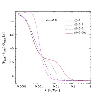
Figure 1: The percentage suppression in matter power spectrum in dark energy models in comparison to $\Lambda$CDM model is plotted for a constant equation of state $w$ and for different values of $c_{e}^{2}$. The left panel is for $w=-0.9$ and right panel shows suppression for $w=-0.8$. It can be seen that suppression is more for dark energy models with $w=-0.8$ with respect to $w=-0.9$. The power spectrums shown in this figure corresponds to its value at the present epoch.

V Suppression of CDM power spectrum

Our aim in this paper is to investigate how perturbations in the dark energy influence the CDM matter power spectrum. In particular, we are interested in models of dark energy whose speed of sound is epoch dependent. In the preceding section, it was illustrated that it is possible to reconstruct the Lagrangian density of the form $\mathcal{L}(X,\phi)=F(X)-V(\phi)$ from a given evolution of the EOS and ESS parameters. Hence, in principle, it is always possible to associate $F(X)$ and $V(\phi)$ for a given evolution of $c_{e}^{2}(a)$ and $w(a)$. This allowed us to choose a parameterized form of $c_{e}^{2}(a)$ and $w(a)$ for which the evolution of perturbations can be investigated. But, before proceeding to the case where $c_{e}^{2}(a)$ is epoch dependent, we will first discuss the case where it is constant.

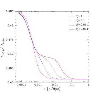
Figure 2: Plot shows the ratio of the percentage suppression in matter power spectrum $\Delta$ defined in Eq. (48) for $w=-0.9$ to $w=-0.8$, for different values of effective speed of sound.

Case I: Constant $c_{e}^{2}$ and $w$

Considering the class of scalar field dark energy models with Lagrangian density of the form $\mathcal{L}(X,\phi)=F(X)-V(\phi)$, if both $w$ and $c_{e}^{2}(a)$ are constants, it follows from Eqs.(44) and (47) that $X(a)\propto a^{n_{1}}$ and $F(a)\propto a^{n_{2}}$, where $n_{1}$ and $n_{2}$ are constants. Therefore, when both $w$ and $c_{e}^{2}(a)$ are constants, the functional form of the kinetic function $F(X)$ would become Mukhanov-2006

$$F(X)=X^{\alpha}$$

where $\alpha$ is a constant given by

$$\alpha=\frac{1-c_{e}^{2}}{2c_{e}^{2}}.$$

It should be noted that for models with $F(X)=X^{\alpha}$, the ESS parameter $c_{e}^{2}$ is always constant irrespective of the functional form of the potential $V(\phi)$ and $w(a)$. It is the form of the potential which would lead to a constant value for the equation of state parameter. The form of the potential can be numerically determined from Eqs.(43) and (45).

In order to determine how CDM perturbation grows when both $c_{e}^{2}$ and $w$ are constants, we numerically solve the closed set of equations (32) to (34), which takes into account the role played by the perturbations in dark energy. Once the evolution of $\Phi(a)$, $\delta_{d}(a)$ and $\sigma_{d}(a)$ is known, the growth of CDM perturbations can be determined using equation (35). For quantifying the difference in the growth of CDM perturbation in dark energy models with respect to $\Lambda$CDM model, we numerically evaluate the following quantity

$$\Delta\%\equiv\frac{P_{{}_{QCDM}}(k)-P_{{}_{\Lambda CDM}}(k)}{P_{{}_{\Lambda CDM}}(k)}\times 100$$ (48)

where $P_{{}_{QCDM}}(k)$ is the CDM power spectrum at the present epoch in dark energy models whereas $P_{{}_{\Lambda CDM}}(k)$ is the corresponding power spectrum in $\Lambda$CDM model. This quantity for the case of constant $c_{e}^{2}$ and $w$ is plotted in Fig. 1. It is clear from this figure that $\Delta$ is negative at all length scales of perturbations. Therefore, CDM power spectrum is suppressed in dark energy models as compared to the same in $\Lambda$CDM model.

The degree of suppression in CDM power spectrum depends on the value of $w$ and $c_{e}^{2}$ and on the length scale of perturbation. In Fig. 1, we have plotted the percentage suppression $\Delta\%$ for $w=-0.9$ and $w=-0.8$ and for different value of constant $c_{e}^{2}$. It follows from this figure that there is more suppression if $w=-0.8$ than if $w=-0.9$, indicating the fact that the degree of suppression is in a way proportional to the deviation of $w$ from $-1$. When comparing percentage suppression for $w=-0.8$ and $w=-0.9$ in Fig. 1, it may appear that they differs just by a factor which is independent of $c_{e}^{2}$. However, this is not true as illustrated by Fig. 2, where we have plotted the ratio of $\Delta$ (defined in Eq.(48)) for $w=-0.8$ and $w=-0.9$. This ratio does depend on the value of $c_{e}^{2}$ clarifying the fact that the percentage suppression $\Delta$ is not merely a product of two functions with one depending on $w$ and the other on $c_{e}^{2}$.

Further, for any value of $w$ and $c_{e}^{2}$, the percentage suppression decreases with increasing length scale of perturbations. This statement is true for the case of constant $w$, however, in general, it depends on the functional form of the equation of state parameter $w(a)$.

It can also be observed from Fig. 1 that the effect of different values of $c_{e}^{2}$ (assumed to be constant) for a given value of $w$ on the CDM power spectrum is insignificant on scales much smaller than the Hubble radius. This statement is also true for scales much larger than the Hubble radius. In fact, it can be be seen from Fig. 1 that only at the intermediate scales, say at $k=0.01h/Mpc$, the effect of different $c_{e}^{2}$ is more pronounced. At these scales, it turns out that the percentage suppression increases with the increase in the value of $c_{e}^{2}$. The reason for the fact that the effect of different values of $c_{e}^{2}$ is significant only at the intermediate scales will be discussed in detail in the next section (Sec.VI).

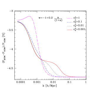
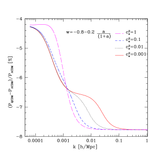
Figure 3: Figure showing suppression in matter power spectrum compared to $\Lambda$CDM model for the case when $w$ is evolving, but $c_{e}^{2}$ is constant. In the left panel, $w$ is initially $-1$ and asymptotically approaches $-0.8$ whereas in the right panel $w$ is initially $-0.8$ and asymptotically approaches $-1$. It can also be verified that in both the panel $w$ at the present epoch is $-0.9$.

Case II: Constant $c_{e}^{2}$ and evolving $w$

When $c_{e}^{2}$ is constant, it is in general possible that the equation of state parameter is epoch dependent. We will now consider such a case. As mentioned earlier, for models with $F(X)=X^{\alpha}$, $c_{e}^{2}$ is always a constant. In fact, it is the form of the potential $V(\phi)$ in these models which determines the evolution of the EOS parameter. We consider the following parametrization for the evolution of $w(a)$,

$$w(a)=w_{0}+w_{1}\left(\frac{a}{1+a}\right)^{n}$$ (49)

where $w_{0}$, $w_{1}$ and $n$ are constants. The constant $w_{0}$ correspond to the initial value of the equation of state parameter (at $a=0$). Asymptotically the equation of state parameter approaches the value $w_{0}+w_{1}$. The parameter ‘$n$’ describes the rate at which $w$ evolves from its initial value $w_{0}$ to its asymptotic value $w_{0}+w_{1}$. The value of $w(a)$ at the present epoch would be $w_{0}+(w_{1}/2^{n})$. Hence, greater the value of $n$ slower will the evolution $w$ from $w_{0}$ to its asymptotic value $w_{0}+w_{1}$.

The parametrization Eq.(49) is different from the one generally investigated in the literature, viz. the Chevallier-Polarski-Linder (CPL) parametrization Chevallier-2001 ; Linder-2003 where $w(z)=w_{0}+w_{{}_{a}}\left(\frac{z}{1+z}\right)$. However, at low red shifts the functional form of both the parametrization converges. Although, the CPL parametrization is very well valid for the range of red shifts which is observationally relevant, it does not restrict the value of $w$ to less than unity. In fact in CPL parametrization, the equation of state parameter diverges asymptotically. This problem does not arise in the parametrization of $w(a)$ introduced in Eq.(49).

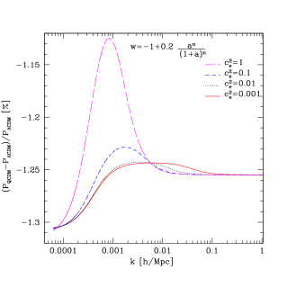
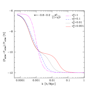
Figure 4: Figure showing suppression in matter power spectrum for $w(a)$ given by Eq.(49) with $n=10$. In the left panel the equation of state parameter is initially $-1$ and stays close to it most of the time whereas in the right panel it evolves from $-0.8$. If one compares the suppression at two length scales say at $k=0.1h/Mpc$ and at $k=0.0001h/Mpc$, it turns out that suppression is more at larger scale compared to small scales in the left panel of this figure. The situation is exactly reverse in the plot on the right panel. This illustrates the fact that the behavior of the suppression at these scales precisely depends on the functional form of $w(a)$.

For constant value of $c_{e}^{2}$, we assume that $w(a)$ evolves with scale factor with the functional form given in Eq.(49). In order to study the effect on matter power spectrum by the dark energy perturbation, we consider two specific behaviors of $w(a)$: one in which $w(a)$ is initially -1 and approaches a constant value ($w>-1$) asymptotically. The other case of interest is where $w>-1$ initially, but asymptotically approaches -1. For the case where $w$ is initially -1 we choose $w_{0}=-1$ and $w_{1}$ to be 0.2, such that asymptotic value of $w=-0.8$. The range of $w$ between -1 and -0.8 is well within the observable constraint on the value of $w$. The second case of interest where $w$ decreases with time and finally approaches -1 would require $w_{0}+w_{1}=-1$. We assume that initially $w=-0.8$, therefore $w_{1}$ would be -0.2.

The suppression of CDM power spectrum as compared to the $\Lambda$CDM in these two cases is shown in Fig.3 for value $n=1$ in Eq.(49). As in the case of constant of $w$ and $c_{e}^{2}$, here also we see that there is a suppression at all scales. The suppression is more in the case when $w=-0.8$ initially (around 8 percent) than the case where $w$ is initially -1. Again it can be seen from Fig. 3 the effect of different values $c_{e}^{2}$ on the suppression is more pronounced at intermediate values of comoving wavenumber $k$.

In the above cases we have chosen the parameter $n$ in Eq.(49) to be unity. If we increase $n$ to 10, then the rate at which EOS parameter switches its value from initial value to the asymptotic value $w_{0}+w_{1}$ slows down dramatically. This case is shown in the Fig.4. When $n=10$, the equation of state parameter for most the time stays near its initial value. Therefore, if $w_{0}=-1$, then it nearly mimic $\Lambda$CDM model for most of evolution, but deviates from it at the present epoch. The peculiar behavior of the suppression in the CDM power spectrum in this case is shown in the left panel in Fig.4. Also we note from this plot that the suppression is very minimal in this case and contrary to other cases the suppression is maximum at small $k$’s than large values of $k$. This peculiar behavior is due to the choice of the function $w(a)$.

The right panel of Fig.4 shows the other case where $w$ is initially -0.8 and approaches -1, the percentage suppression in this case is high for the obvious reason that $w$ for most of the time stays close to $-0.8$. Also it should be noted that suppression in this case is larger at smaller length scales unlike the case in the left panel. This illustrates the fact that the percentage suppression at both smaller and larger scales very much depends on the functional form of the equation of state parameter $w(a)$. It should also be noted that the effect of different values of $c_{e}^{2}$ can be seen more profoundly only at the intermediate scales.

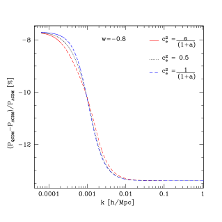
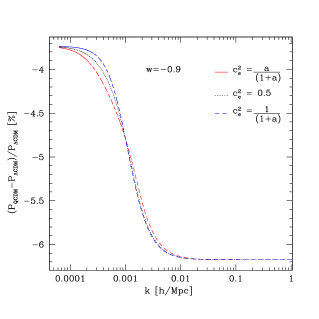
Figure 5: The behavior of suppression in matter power spectrum as compared to $\Lambda$CDM model for the case when EOS parameter $w$ is constant but ESS parameter $c_{e}^{2}$ is evolving with scale factor is shown in this figure. The left panel shows the case when $w=-0.8$ whereas the right panel show for $w=-0.9$. The suppression in matter power spectrum for the case when $c_{e}^{2}$ asymptotically decays to zero from its initial value of unity is compared with the reverse case where it increases to unity from zero. For comparison $c_{e}^{2}=0.5$ is also plotted. Note that in all these cases the value of $c_{e}^{2}$ at the present epoch is $0.5$

Case III: constant $w$ and evolving $c_{e}^{2}$

Let us now consider the case of dark energy models for which EOS parameter $w$ is constant but $c_{e}^{2}$ evolves with time. As mentioned earlier, the class of dark energy models described by the lagrangian density (36) does allow $c_{e}^{2}$ to evolve with time when $w$ is constant. It should be noted that this is not in general valid for all classes of scalar field DE models. For example in tachyon model of DE with $\mathcal{L}_{1}=V(\phi)\sqrt{1-2X}$, a constant $w$ always implies that $c_{e}^{2}$ is also constant.

We consider the following parametrization for the evolution of $c_{e}^{2}$ with the scale factor

$$c_{e}^{2}=c_{0}+c_{1}\left(\frac{a}{1+a}\right)^{n}$$ (50)

This is similar to the parametrization of $w$ discussed in the preceding section (see Eq.(49)). The interpretation of the constants $c_{0}$ and $c_{1}$ in Eq.(50) is as follows. The constant $c_{0}$ corresponds to the initial value of the ESS parameter $c_{e}^{2}$, whereas $c_{0}+c_{1}$ corresponds to its asymptotic value. The parameter $n$ determines the rate at which the ESS parameter evolves from $c_{0}$ to its asymptotic value $c_{0}+c_{1}$.

We are interested in comparing the suppression in CDM power spectrum with respect to $\Lambda$CDM in cases where $c_{e}^{2}$ decreases with time with those where it increases. For the increasing case we choose $c_{0}=0$ and $c_{1}=1$ so that $c_{e}^{2}$ evolves from $0$ to 1 asymptotically. Similarly for the decreases case we choose $c_{0}=1$ and $c_{1}=-1$ so that $c_{e}^{2}$ evolves from $1$ to $0$. The suppression of CDM power spectrum for these cases with n = 1 in Eq.(50) is shown in Fig.5. This choice of these set of parameters ensures that the value $c_{e}^{2}$ at the present epoch for these two cases is the same and is given by $0.5$. Hence, for comparison the case of constant $c_{e}^{2}$ with $c_{e}^{2}=0.5$ is also plotted in the same figure. It is interesting to note that the three curves in Fig.5 (both left and the right panel) almost overlap with each other indicating the fact that the effect of different evolution of $c_{e}^{2}(a)$ for a constant $w$ is insignificant on the suppression of CDM power spectrum. This may not be true for any evolution of $c_{e}^{2}$ with the scale factor.

In order to check the generality of this result we consider two more different evolution of $c_{e}^{2}$. The first one is the same function introduced in Eq.(50) with the following values of the parameter $c_{0}=10^{-5}$, $c_{1}=1$ and $n=10$. In this case $c_{e}^{2}(a)$ evolves from $c_{0}=10^{-5}$ initially to $10^{-3}$ at the present epoch. The second functional form of $c_{e}^{2}(a)$ we consider is $c_{e}^{2}(a)=1/(1+a)^{n}$ with $n=10$. Here, in this case $c_{e}^{2}(a)$ evolves from its initial value of unity to $10^{-3}$ at the present epoch. The suppression of CDM power spectrum in these two cases is shown in Fig.6 It is evident from this figure that the two curves are not as close to each other as compared to the three curves in Fig.5. The reason for this is that in these two curves order of magnitude change in $c_{e}^{2}$ from $z=1000$ to present epoch is much larger than the cases presented in Fig.5. However, it should be noted that, as in the previous cases of constant $c_{e}^{2}$ the effect of different choice of $c_{e}^{2}(a)$ on CDM power spectrum is not evident at large and low values of $k$.

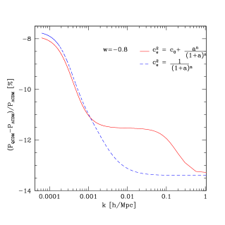
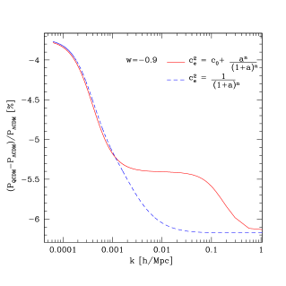
Figure 6: Comparison of suppression of matter power spectrum for two different evolution of $c^{2}_{e}(a)$ with scale factor is shown in this Fig. Here we have taken $c_{0}=10^{-5}$ and $n=10$. For both these curves it can be verified that the present value of $c^{2}_{e}$ is approximately $10^{-3}$.

Case IV: Evolving $w$ and $c_{e}^{2}$

Until now we have considered the cases where both $w$ and $c_{e}^{2}$ are constants and the case where either one of them is epoch dependent. For the purpose of completeness, we now consider the case where both $w$ and $c_{e}^{2}$ evolves with time. This is the most general case and in reality, for k-essence models, it is likely that these two parameters are epoch dependent.

We will study two cases, first with the following evolution of $w(a)=-1+0.2\left(\frac{a}{1+a}\right)$, and the two functions $c_{e}^{2}=\left(\frac{a}{1+a}\right)$ and $c_{e}^{2}=\left(\frac{1}{1+a}\right)$. The choice of $w(a)$ corresponds to the case where it evolves from $-1$ to $-0.9$ at the present epoch The second case we consider is with the same two functional form of $c_{e}^{2}$ but with $w(a)$ given by $w(a)=-0.8-0.2\left(\frac{a}{1+a}\right)$ is initially -0.8 and evolves to $-0.9$ at the present epoch. The suppression of CDM power spectrum as compared to $\Lambda$CDM model in these two cases are shown in the Fig.7. it is evident from this figure that the behavior of suppression with $k$ is similar in the both cases, with suppression being maximum at the smaller scales than at larger scales. Also it is clear from the two figures that suppression is more in the case where $w$ is initially $-0.8$ than the case where initial value is -1, reiterating the point that as we move away from value of $w=-1$ the the effect of dark energy perturbations is more important. Finally, we infer that for different functional form of $c_{e}^{2}(a)$ for a given evolution of $w(a)$ does not have any considerable effect on the matter power spectrum. In fact it can be observed from Fig.7 that changing the functional form of $w(a)$ for a given evolution of $c_{e}^{2}(a)$ influences the matter power spectrum more severely than the reverse case.

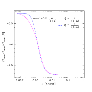
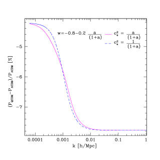
a b

Figure 7: Supression in matter power spectrum as compared to that in $\Lambda$CDM model in the case when both $c_{e}^{2}$ and $w$ are epoch dependent. In the left panel we have chosen a form of $w(a)$, which is initially $-1$ and asymptotically goes to a constant value $-0.8$ and in the right panel $w$ is chosen such that it is initially $-0.8$ and asymptotically approaches $-1$.

VI The role of perturbation in dark energy

From the discussions in the preceding section, it follows that for a given evolution $w(a)$, the effect of different functional form of $c_{e}^{2}$ on the CDM power spectrum is significant only at the intermediate scales (see Fig.1 to Fig.7). In fact, at scales much smaller (or larger) than the Hubble radius, the suppression of CDM power spectrum with respect to the $\Lambda$CDM model is nearly independent of the functional form of $c_{e}^{2}(a)$. The reason for this behavior is discussed in this section.

At the sub-Hubble scales

At scales much smaller than the Hubble radius, the perturbation in dark energy is negligibly smaller than the corresponding perturbation in dark matter Sanil-2008a . This result follows from the numerical solutions of Eqs.(32) to (34). In Fig.8, we have plotted the ratio $\delta_{d}/(1+w)\delta_{m}$ at the present epoch for different length scales of perturbations. It follows from this figure that at scales much smaller than the Hubble radius ($k>>0.001h/Mpc$), the perturbation in dark energy is negligibly smaller in comparison to that in dark matter. In fact, at these scales it can be assumed that the dark energy is homogeneously distributed.

Since we have assumed dark energy to be a scalar field, homogeneous dark energy at these scales reflects to the fact that scalar field fluctuations at these scales are negligibly smaller than other perturbation variables such as $\delta_{m}$, $\Phi$, etc. With this assumption that the dark energy is homogeneous at scales much smaller than the Hubble radius, it turns out that the evolution of the Bardeen potential $\Phi$ at these scales is governed by the following equation

$$\ddot{\Phi}+4H\dot{\Phi}+\left(2\dot{H}+3H^{2}+3H^{2}\left(\frac{1+w(a)}{2}\right)\Omega_{d}(a)\right)\Phi=0.$$ (51)

The above equation corresponds to the evolution of $\Phi$ in a system of dark matter and homogeneous scalar field dark energy. In the case of $\Lambda$CDM model, the corresponding equation for $\Phi$ is given by

$$\ddot{\Phi}_{\Lambda}+4H\dot{\Phi}_{\Lambda}+\left(2\dot{H}+3H^{2}\right)\Phi_{\Lambda}=0.$$ (52)

This evolution equation for $\Phi$ in $\Lambda$CDM model is valid at all length scales. However, it should be noted that Eq.(51) is strictly valid only at scales much smaller than the Hubble radius where dark energy can be assumed to be homogeneous. At these scales, the perturbation in dark matter is given by

$$\delta_{m}=-\left(\frac{1}{4\pi G\,\bar{\rho}_{m}(a)}\right)\frac{k^{2}}{a^{2}}\Phi$$ (53)

Therefore, the percentage suppression in CDM power spectrum due to dark energy in comparison to $\Lambda$CDM model ($\Delta\%$ defined in Eq.(48)) would become

$$\Delta\%=\frac{\Phi^{2}-\Phi_{\Lambda}^{2}}{\Phi_{\Lambda}^{2}}\times 100$$ (54)

From the numerical solution of Eqs.(51) and (52), it follows that for $w=-0.8$, the value of $\Delta\%$ is $-13.39$ whereas for $w=-0.9$, it turns out to be $-6.17$. These values matches with the one shown in Fig.1 at $k>>0.001h/Mpc$, which was plotted without assuming a priori the homogeneity of dark energy at these scales.

The evolution of Bardeen potential $\Phi$ at scales much smaller than the Hubble radius is independent of $c_{e}^{2}$ (see Eq.(51)). The corresponding growth of CDM perturbation at these scales given by Eq.(53) is also independent of $c_{e}^{2}$. Therefore, at these scales the suppression in CDM power spectrum is independent of the dark energy speed of sound $c_{e}^{2}$. As emphasized earlier, the primary reason for this is the fact that at these scales dark energy is nearly homogeneous. It is only through the perturbation in dark energy that $c_{e}^{2}$ plays a role in suppressing the CDM power spectrum compared to that in $\Lambda$CDM model.

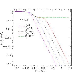
Figure 8: The raio of perturbation in dark energy to the perturbation in dark matter scaled by a factor $1/(1+w)$ is plotted in this figure. It can be observed that at length scales much larger than the Hubble radius this ratio approaches unity. The reason for this is that at these scales the incurvature perturbation vanishes. Therefore, at these scales $\delta_{d}=(1+w)\delta_{m}$.

At the super-Hubble scales

At scales comparable to Hubble radius and beyond ($k<0.001h/Mpc$), the perturbation in dark energy cannot, in general, be neglected in comparison to that in dark matter. This evident from Fig.8, which shows that in the limit $k<<0.001h/Mpc$, the perturbation in dark energy becomes

$$\delta_{d}=(1+w)\delta_{m}$$ (55)

If $w\neq-1$, then perturbation in dark energy can become comparable to that in matter at these scales ($k<0.001h/Mpc$). Eq.(55) also follows from the fact that at these scales, the isocurvature perturbation or the total non-adiabatic pressure perturbation vanishes. In addition to this, the intrinsic entropy perturbation of dark energy also vanishes at these scales. The intrinsic entropy perturbation of dark energy is proportional to its non-adiabatic pressure perturbation defined as

$$\delta p_{{}_{nad}}=\delta p_{d}-c_{a}^{2}\delta\rho_{d}$$ (56)

For scalar field dark energy, it $\delta p_{{}_{nad}}$ can also be expressed as

$$\delta p_{{}_{nad}}=(c_{e}^{2}-c_{a}^{2})\left[\delta_{d}-3H^{2}(1+w)a^{2}u_{d}\right]\bar{\rho}_{d}(a).$$ (57)

At the super Hubble scales, the $\delta p_{{}_{nad}}$ of dark energy vanishes not because of the fact that $c_{e}^{2}=c_{a}^{2}$ but because

$$\delta_{d}=3H^{2}(1+w)a^{2}u_{d}$$ (58)

In fact, it can be verified that in the limit $k\rightarrow 0$, Eqs.(55) and (58) are consistent with the covariant conservation equation for dark matter and dark energy.

With the fact that the non-adiabatic pressure perturbation of dark energy vanishes at scales much larger than the Hubble radius, it turns out that the evolution of Bardeen potential at these scales is governed by the following equation

$$\ddot{\Phi}+\left(4+3c_{a}^{2}(1+w)\left(\frac{\Omega_{d}(a)}{1+w(a)\Omega_{d}(a)}\right)\right)H\dot{\Phi}+\left(2\dot{H}+3H^{2}+3H^{2}c_{a}^{2}(1+w)\left(\frac{\Omega_{d}(a)}{1+w(a)\Omega_{d}(a)}\right)\right)\Phi=0.$$ (59)

The evolution of $\Phi$ in $\Lambda$CDM model follows from the above equation if we substitute $w=-1$. In the limit $k<<0.001h/Mpc$, neglecting the $k^{2}$ term in time-time linearized Einstein’s equation ($\delta G^{0}_{\hskip 5.69046pt0}=8\pi G\,\delta T^{0}_{\hskip 5.69046pt0}$,) together with the fact that $\delta_{d}=(1+w)\delta_{m}$, it turns out that the equation for $\delta_{m}$ becomes

$$\delta_{m}=\left(\frac{-2}{1+w(a)\Omega_{d}(a)}\right)\left(\Phi+\frac{\dot{\Phi}}{H}\right)$$ (60)

The percentage suppression in CDM power spectrum can now be evaluated by numerically solving Eq.(59) and then evaluating $\delta_{m}$ using Eq.(60). It turns out $\Delta\%$ defined in Eq.(48) for $w=-0.8$ at these scales ($k\rightarrow 0$) is $-7.7$. and for $w=-0.9$ it becomes $-3.7$. These values are consistent with those in Fig.1 for $k<<0.001h/Mpc$ where we have solved the exact perturbation equation without imposing any assumption.

Hence, at scales much higher than the Hubble radius, the effective speed of sound of dark energy does not influence the CDM perturbations. This is because the intrinsic entropy perturbation of dark energy vanishes at these scales. It is the intrinsic entropy perturbation of dark energy which carries the information of the ESS parameter $c_{e}^{2}(a)$. Thus, it is only at the intermediate scales (scales around $k\sim 0.01h/Mpc$) where the effect of different evolution of $c_{e}^{2}(a)$ is more pronounced on the suppression of CDM power spectrum with respect to $\Lambda$CDM model.

VII Summary and Conclusions

In this paper we have investigated the influence of perturbation in dark energy on the matter power spectrum in models where the effective speed of sound $c_{e}^{2}(a)$ of dark energy evolves with time. We first presented a method of reconstructing the lagrangian density of dark energy of the form $\mathcal{L}(X,\phi)=F(X)-V(\phi)$ from a given evolution of $c_{e}^{2}(a)$ and the equation of state parameter $w(a)$. This illustrates the fact that these scalar field dark energy models, in principle, allows a wide class of solutions with different functional form of $w(a)$ and $c_{e}^{2}(a)$. In fact, in these models evolution in $c_{e}^{2}(a)$ can be independent of that in $w(a)$.

We then investigated the growth of CDM perturbation as influenced by the perturbations in dark energy in models where $(i)$ both $c_{e}^{2}$ and $w$ are constants, $(ii)$ either of them are epoch dependent and $(iii)$ both of them are epoch dependent. It is shown that in all these cases, the CDM power spectrum is generically suppressed in comparison to that in $\Lambda$CDM model. The degree of suppression at different length scales does in fact depend on the behavior of $w(a)$ and $c_{e}^{2}(a)$.

When the equation of state parameter of dark energy is constant, it is shown that the percentage suppression in CDM power spectrum with respect to the $\Lambda$CDM model decreases with increasing length scale of perturbation (see Fig.1). However, this is not generically true for any evolution of $w(a)$. In fact, it is found that for slow evolution of $w(a)$ from $-1$ to a value close to it (with $w+1>0$), the percentage suppression in CDM power spectrum can increase with increase in the length scale of perturbation (see, left panel of Fig.4).

Primarily, in this paper we have compared the percentage suppression in CDM power spectrum in dark energy models where its effective speed of sound $c_{e}^{2}(a)$ increases with scale factor with those where it decreases. It is shown that the effect of different evolution of $c_{e}^{2}(a)$ of dark energy on the matter power spectrum for a given evolution of equation of state parameter $w(a)$ is not as much significant as compared to the reverse case, viz. different evolution of $w(a)$ for a given evolution of $c_{e}^{2}(a)$ (as shown in Fig.5 to Fig.7). This illustrates the fact that the effect of equation of state parameter $w(a)$ of dark energy on the CDM power spectrum is much more severe than its effective speed of sound $c_{e}^{2}(a)$.

Further, it is also shown that the effect of different evolution of $c_{e}^{2}(a)$ for a given evolution of $w(a)$, on the suppression of CDM power spectrum is more pronounced only at the intermediate scales at around $k\sim 0.01h/Mpc$. In fact it is observed that the degree of suppression of CDM power spectrum with respect to $\Lambda$CDM model is nearly independent of $c_{e}^{2}(a)$ at scales much smaller and larger than the Hubble radius. The reason for this behavior at scales much smaller than the Hubble radius is as follows. At these scales, it turns out that the perturbation in dark energy is negligibly smaller than the corresponding perturbation in matter. One can effectively approximate dark energy to be homogeneous at these scales. Since it is the perturbation in dark energy which carries the information of its effective speed of sound, the suppression of CDM power spectrum at these scales will be independent of any functional form of $c_{e}^{2}(a)$. The suppression at these scales will primarily be governed by the functional form of $w(a)$ of dark energy.

Even at scales much larger than the Hubble radius, suppression of CDM power spectrum with respect to $\Lambda$CDM model is nearly independent of $c_{e}^{2}(a)$. At these scales the perturbation in dark energy cannot be neglected in comparison to matter perturbation if $w(a)$ deviates from $-1$ (as shown in Fig.8). However, it is found that at these scales both the total entropy perturbation (or the isocurvature perturbation) and the intrinsic entropy perturbation of dark energy vanishes. It is in fact the intrinsic entropy perturbation of dark energy which encodes the information of its effective speed of sound. Therefore, at these scales, although there is dark energy perturbation, it is purely adiabatic and consequently its effect on the suppression of CDM power spectrum will be same for different $c_{e}^{2}(a)$.

In summary, it is illustrated in this paper that the suppression of CDM power spectrum with respect to $\Lambda$CDM model both at scales much larger and smaller than the Hubble radius only depends on the form of $w(a)$ of dark energy. It is only at the intermediate scales, a non zero value of the effective speed of sound of dark energy leaves its imprint on the CDM power spectrum. Precisely determining the effective speed of sound of dark energy, although observationally challenging Putter-2010 , is necessary to understand its nature. We hope that future observations will shed more light on the ‘darkness’ of the dark energy.

References

- (1) A. G. Riess et al., Astron. J. 116, 1009 (1998).
- (2) S. Perlmutter et al., Astrophys. J. 517, 565 (1999).
- (3) D. N. Spergel et al., Astrophys. J. Suppl. Ser. 170, 377 (2007).
- (4) E. Komatsu et al., Astrophys. J. Suppl. 180, 330, (2009).
- (5) E. Komatsu et al., Astrophys. J. Suppl. 192, 18, (2011).
- (6) T. Padmanabhan, Phys. Rep. 380, 235 (2003).
- (7) V. Sahni, Lecture Notes in Physics (Springer Verlag, Berlin, Germany, 2004)
- (8) E. J. Copeland, M. Sami, S. Tsujikawa, Int. J. Mod. Phys. D 15, 1753 (2006).
- (9) V. Sahini and A. Starobinsky, Int. J. Mod. Phys. D 15,2105, (2006).
- (10) T. Padmanabhan, Phys. Rev. D 66, 021301 (2002).
- (11) A. Feinstein, Phys. Rev. D 66, 063511 (2002).
- (12) S. Unnikrishnan, Phys. Rev. D 78, 063007, (2008).
- (13) W. Hu, Phys. Rev. D 65, 023003, (2001).
- (14) J. K. Erickson, R. R. Caldwell, P. J. Steinhardt, C. A. Picon, and V. Mukhanov, Phys. Rev. Lett. 88, 121301 (2002).
- (15) J. Weller, and A. M. Lewis, Mon. Not. R. Astron. Soc. 346, 987 (2003).
- (16) S. DeDeo, R. R. Caldwell, and P. J. Steinhardt, Phys. Rev. D 67, 103509, (2003).
- (17) R. bean, and O. Dore, Phys. Rev. D 69, 083503 (2004).
- (18) C. Gordon, and W. Hu, Phys. Rev. D 70, 083003, (2004).
- (19) C. Gordon, and D. Wands, Phys. Rev. D 71, 123505, (2005).
- (20) P-S. Corasaniti, T. Giannantonio, and A. Melchiorri, Phys. Rev. D 71, 123521, (2005).
- (21) S. Hannestad, Phys. Rev. D 71, 103519, (2005).
- (22) L. R. Abramo, R. C. Batista, L. Liberato, and R. Rosenfeld, JCAP 11, 012 (2007).
- (23) S. Unnikrishnan, H. K. Jassal, and T. R. Seshadri, Phys. Rev. D 78, 123504, (2008).
- (24) G. Ballesteros, and A. Riotto, Phys. Lett. B 668, 171 (2008).
- (25) V. Gorini, A. Y. Kamenshchik, U. Moschella, O. F. Piattella, and A. A. Starobinsky, JCAP 02, 016 (2008).
- (26) C-G. Park, J. Hwang, J.Lee, and H. Noh, Phys. Rev. Lett. 103, 151303 (2009).
- (27) J. B. Dent, S. Dutta, and T. J. Weiler, Phys. Rev. D 79, 023502, (2009).
- (28) L. R. Abramo, R. C. Batista, and R. Rosenfeld, JCAP 07, 040 (2009).
- (29) H. K. Jassal, Phys. Rev. D 79, 127301, (2009).
- (30) D. Sapone and M. Kunz, Phys. Rev. D 80, 103505, (2009).
- (31) O. Sergijenko and B. Novosyadlyj, Phys. Rev. D 80, 083007, (2009).
- (32) H. K. Jassal, Phys. Rev. D 81, 083513, (2010).
- (33) R. de Putter, D. Huterer, and E. V. Linder, Phys. Rev. D 81, 103513, (2010).
- (34) J. C. B. Sanchez and L. Perivolaropoulos, Phys. Rev. D 81, 103505, (2010).
- (35) G. Ballesteros and J. Lesgourgues, JCAP, 1010, 014, (2010).
- (36) K. Karwan, JCAP 02, 007 (2011).
- (37) J. Bardeen, Phys. Rev. D 22, 1882 (1980).
- (38) H. Kodama and M. Sasaki, Prog. Theor. Phys. Suppl. 78, 1 (1984)
- (39) V. F. Mukhanov, H. A. Feldman and R. H. Brandenberger, Phys. Rep. 215, 203 (1992)
- (40) W. Hu, Astrophys. J. 506, 485 (1998).
- (41) S. Unnikrishnan, and L. Sriramkumar, Phys. Rev. D 81, 103511 (2010).
- (42) J. Garriga and V. F. Mukhanov, Phys. Lett. B 458, 219 (1999).
- (43) C. Armenda riz-Pico n, T. Damour, and V. F. Mukhanov, Phys. Lett. B 458, 209 (1999).
- (44) W. Hu, Phys. Rev. D 71, 047301 (2005).
- (45) V. Mukhanov and A. Vikman, JCAP 02, 004 (2006).
- (46) M. Chevallier and D. Polarski, Int. J. Mod. Phys. D 10, 213 (2001).
- (47) E. V. Linder, Phys. Rev. Lett. 90, 091301 (2003).