Tree-Structured Random Vector Quantization for Limited-Feedback Wireless Channels

Abstract

We consider the quantization of a transmit beamforming vector in multiantenna channels and of a signature vector in code division multiple access (CDMA) systems. Assuming perfect channel knowledge, the receiver selects for a transmitter the vector that maximizes the performance from a random vector quantization (RVQ) codebook, which consists of independent isotropically distributed unit-norm vectors. The quantized vector is then relayed to the transmitter via a rate-limited feedback channel. The RVQ codebook requires an exhaustive search to locate the selected entry. To reduce the search complexity, we apply generalized Lloyd or $k$-dimensional (kd)-tree algorithms to organize RVQ entries into a tree. In examples shown, the search complexity of tree-structured (TS) RVQ can be a few orders of magnitude less than that of the unstructured RVQ for the same performance. We also derive the performance approximation for TS-RVQ in a large system limit, which predicts the performance of a moderate-size system very well.

I Introduction

Channel information at both the transmitter and receiver can increase the performance of wireless systems significantly. With channel information, the transmitter can adapt its transmit power and waveform to a dynamically fading channel while the receiver can detect transmit symbols from received signals. Typically, channel information can be estimated at the receiver from pilot signals during a training period. The transmitter on the other hand is usually not able to directly estimate a forward channel, especially in a frequency division duplex where a channel in one direction is not reciprocal to that in the opposite direction. Thus, the transmitter has to rely on the receiver for channel information. Normally, the receiver relays channel information to the transmitter via a rate-limited feedback channel.

The receiver can directly quantize channel coefficients and feeds back the quantized coefficients to the transmitter, which adapts its transmission, accordingly [1]. Alternatively, the receiver computes and quantizes the optimal transmit coefficients. References [2, 3, 4, 5, 6] proposed quantization of the transmit precoding matrix, which consists of transmit antenna weights in a multiantenna channel while [7, 8] considered quantization of the signature vector in CDMA. Comparing the two approaches, [1] showed that quantizing transmit coefficients performs much better than direct channel quantization.

Most of the proposed quantization codebooks require an exhaustive search to locate the quantized signature vector. The search complexity depends on the number of entries in the quantization codebook, which grows exponentially with available feedback bits denoted by $B$. Reducing the search complexity while not jeopardizing the performance is desirable. In [7], the number of coefficients to be quantized was reduced by projecting the signature vector onto a lower dimensional subspace and the coefficients were then scalar quantized. Although the complexity of scalar quantization is much less than that of vector quantization, the performance of the scalar quantization scheme suffers greatly. References [9, 10] proposed a search algorithm for the QAM codebook, which is based on a noncoherent detection algorithm [11]. The associated complexity grows linearly with $B$ with small performance loss. However, the algorithm is not applicable when $B$ is smaller than the number of coefficients. To reduce the search complexity, we propose to organize an unstructured random vector quantization (RVQ) codebook into a tree by either a generalized Lloyd (GLA) algorithm [12, 13] or a $K$-dimensional (kd) tree algorithm [14, 15]. The tree-building process is computationally complex, but can be performed offline. An RVQ codebook was proposed in [6, 7] and contained independent isotropically distributed unit-norm vectors. For moderate-size systems, RVQ performs close to the optimum codebook designed for a channel with independent identically distributed gains. In a large system limit in which system parameters tend to infinity with fixed ratios, RVQ is optimal [6, 7] (i.e., maximizing capacity or minimizing interference power).

In this work, we consider quantizing both the transmit beamforming vector in multi-input multi-output (MIMO) channel and the signature sequence in reverse-link CDMA. With a tree-structured (TS) RVQ codebook, the receiver searches the tree for the vector that is closest in Euclidean distance to the optimal unquantized signature vector, which is the eigenvector of the received covariance matrix. We note that the obtained quantized vector may not give the optimal performance (i.e, maximizing received power in a MIMO channel or minimizing the interference power in CDMA). However, the performance loss incurred is small when $B$ is large, while the corresponding search complexity is reduced by a few orders of magnitude from that of a full search. For smaller $B$, the performance, however, takes a significant loss. So, we modify the kd-tree search algorithm to narrow the performance gap. Analyzing the performance of the TS-RVQ codebook is not tractable. Hence, we derive the performance approximation of the TS-RVQ codebook in the large system limit. The derived approximation is a function of the number of feedback bits per degree of freedom and the normalized load and is shown to predict the performance of a system with moderate-to-large size very well.

II System Model

We are interested in two wireless channel models as follows.

II-A Point-to-Point Multiantenna Channel

We first consider a discrete-time point-to-point channel with $N_{t}$ transmit antennas and $N_{r}$ receive antennas. The $N_{r}\times 1$ received vector is given by

$$\bm{r}=\bm{H}\bm{v}b+\bm{n}$$ (1)

where $\bm{H}=[h_{n_{r},n_{t}}]$ is an $N_{r}\times N_{t}$ channel matrix, $\bm{v}$ is an $N_{t}\times 1$ beamforming unit-norm vector, $b$ is a transmitted symbol, $\bm{n}$ is an $N_{r}\times 1$ additive white Gaussian noise vector with zero mean and covariance $\sigma_{n}^{2}\bm{I}$, and $\bm{I}$ is an identity matrix. Assuming an ideal rich scattering environment, we model $h_{n_{r},n_{t}}$ as a complex Gaussian random variable with zero mean and variance $1/N_{r}$. Thus, the received fading power is given by $\sum_{n_{r}=1}^{N_{r}}E[|h_{n_{r},n_{t}}|^{2}]=1$ for a given $n_{t}$th transmit antenna. An ergodic channel capacity is given by

$$C(\bm{v})=E_{\bm{H}}[\log(1+\rho\bm{v}^{{\dagger}}\bm{H}^{{\dagger}}\bm{H}\bm{v})]$$ (2)

where expectation is over distribution of $\bm{H}$, and $\rho=1/\sigma_{n}^{2}$ is the background signal-to-noise ratio (SNR). We note that the capacity (2) is a function of the beamforming vector $\bm{v}$ and that only a rank-one transmit beamforming is considered. Quantization of an arbitrary-rank transmit precoding matrix was studied by [6].

II-B Reverse-Link CDMA

We also examine a reverse-link CDMA with $K$ users and processing gain $N$. User $k$ is assigned the $N\times 1$ signature vector $\bm{s}_{k}$ for $1\leq k\leq K$. The user signal is assumed to traverse $L$ fading paths. We denote the $N\times N$ channel matrix for user $k$ by

$$\bm{C}_{k}=\left[\begin{array}[]{ccccccc}h_{k,1}&0&\ldots&0&0&\ldots&0\\ \vdots&h_{k,1}&&\vdots&0&&\vdots\\ h_{k,L}&\vdots&\ddots&0&\vdots&&0\\ 0&h_{k,L}&&h_{k,1}&0&\ldots&0\\ \vdots&0&\ddots&\vdots&h_{k,1}&&0\\ 0&\vdots&&h_{k,L}&\vdots&\ddots&0\\ 0&0&\ldots&0&h_{k,L}&\ldots&h_{k,1}\end{array}\right]$$ (3)

where fading gains for user $k$, $h_{k,1}$, …, $h_{k,L}$ are independent complex Gaussian random variables with zero mean and variance $E|h_{k,1}|^{2}$, …, $E|h_{k,L}|^{2}$, respectively. Here we assume that the symbol duration is much longer than the delay spread and thus, inter-symbol interference is negligible. For an ideal nonfading channel, $\bm{C}_{k}$ = $\bm{I}$ for all $k$.

The $N\times 1$ received vector at the base station is given by

$$\bm{r}=\bm{H}\bm{b}+\bm{n}$$ (4)

where $\bm{b}=[b_{1}\quad b_{2}\ \ldots\ b_{K}]$ is the vector of $K$ users’ transmitted symbols and

$$\bm{H}=[\bm{C}_{1}\bm{s}_{1},\ \ldots\ ,\bm{C}_{K}\bm{s}_{K}].$$ (5)

In this work, we only consider single-user signature quantization. Without loss of generality, we assume that user 1’s signature is quantized while other signatures do not change. Signature quantization for multiple users was considered by [16]. Assuming a matched-filter receiver for user 1

$$\bm{c}_{1}=\frac{\bm{C}_{1}\bm{s}_{1}}{|\bm{C}_{1}\bm{s}_{1}|},$$ (6)

the interference power for user 1 is given by

$$I_{1}\triangleq\sum_{k=2}^{K}(\bm{s}_{1}^{\dagger}\bm{C}_{1}^{\dagger}\bm{C}_{k}\bm{s}_{k})^{2}=\bm{s}_{1}^{\dagger}\bm{C}_{1}^{\dagger}\bm{H}_{1}^{{\dagger}}\bm{H}_{1}\bm{C}_{1}\bm{s}_{1}$$ (7)

where $\bm{H}_{1}=[\bm{C}_{2}\bm{s}_{2}\quad\bm{C}_{3}\bm{s}_{3}\ \ldots\ \bm{C}_{K}\bm{s}_{K}]$ is the $N\times(K-1)$ interfering signature matrix. Hence, the associated output signal-to-interference plus noise ratio (SINR) for user 1 is given by

$$\gamma_{1}(\bm{s}_{1})=\frac{(\bm{s}_{1}^{\dagger}\bm{C}_{1}^{\dagger}\bm{C}_{1}\bm{s}_{1})^{2}}{I_{1}+\sigma_{n}^{2}\bm{s}_{1}^{\dagger}\bm{C}_{1}^{\dagger}\bm{C}_{1}\bm{s}_{1}}.$$ (8)

Similar to MIMO channels, the performance of the CDMA user (8) also depends on the transmit signature vector $\bm{s}_{1}$.

With channel information, the receiver in the MIMO channel selects $\bm{v}$ that maximizes the capacity from an RVQ codebook, which is known a priori at both the transmitter and receiver. The RVQ codebook contains independent and isotropically distributed unit-norm vectors and is denoted by

$$\mathcal{V}=\{\bm{v}_{1},\bm{v}_{2},\ldots,\bm{v}_{2^{B}}\}$$ (9)

where $B$ denotes available feedback bits. RVQ was proposed by [7, 6] and was shown to be optimal in a large system limit in which $(N_{t},N_{r},B)\to\infty$. For CDMA, the receiver selects $\bm{s}_{1}$ that minimizes the interference power for user $1$.

Maximizing the capacity for the MIMO channel in (2) is equivalent to maximizing the received signal power. Thus, the receiver selects

$$\hat{\bm{v}}=\arg\max_{\bm{v}_{j}\in\mathcal{V}}\ \bm{v}_{j}^{{\dagger}}\bm{H}^{{\dagger}}\bm{H}\bm{v}_{j}$$ (10)

for given $\bm{H}$. In CDMA, the receiver selects

$$\hat{\bm{s}}_{1}=\arg\min_{\bm{v}_{j}\in\mathcal{V}}\ \bm{v}_{j}^{{\dagger}}\bm{C}_{1}\bm{H}_{1}^{{\dagger}}\bm{H}_{1}\bm{C}_{1}^{{\dagger}}\bm{v}_{j}$$ (11)

for given $\bm{H}_{1}$ and $\bm{C}_{1}$ to minimize the interference power. As $B$ increases, the number of entries in the codebook increases and so does the performance with the selected signature vector in both (10) and (11). However, the search complexity also grows since the RVQ codebook requires a full search to locate the optimal entry and thus, complexity can pose a serious problem for very large $B$.

III Nearest-Neighbor Search

Let $\bm{S}\bm{S}^{{\dagger}}$ denote a covariance matrix where $\bm{S}$ denotes an $N\times K$ effective signature matrix for both MIMO and CDMA channels. Performing a singular value decomposition (SVD) on the covariance matrix gives

$$\bm{S}\bm{S}^{{\dagger}}=\sum_{i=1}^{N}\lambda_{i}\bm{u}_{i}\bm{u}^{{\dagger}}_{i}$$ (12)

where $\lambda_{1}\leq\lambda_{2}\leq\cdots\leq\lambda_{N}$ are the ordered eigenvalues and $\bm{u}_{i}$ is the corresponding $i$th eigenvector. It is well known that the first eigenvector maximizes the quadratic form $\bm{v}^{{\dagger}}\bm{S}\bm{S}^{{\dagger}}\bm{v}$ as follows

$$\bm{u}_{1}=\arg\max_{\bm{v}}\bm{v}^{{\dagger}}\bm{S}\bm{S}^{{\dagger}}\bm{v}$$ (13)

while the $N$th eigenvector minimizes the quadratic form as follows

$$\bm{u}_{N}=\arg\min_{\bm{v}}\bm{v}^{{\dagger}}\bm{S}\bm{S}^{{\dagger}}\bm{v}.$$ (14)

To quantize these optimal eigenvectors for the transmitter, the receiver may search the given codebook for the vector that is closest in Euclidean distance to either $\bm{u}_{1}$ or $\bm{u}_{N}$ (finding the nearest neighbor). To quantize $\bm{u}_{1}$, the receiver selects

$$\bar{\bm{v}}_{1}\triangleq\arg\min_{\bm{v}_{j}\in\mathcal{V}}\|\bm{u}_{1}-\bm{v}_{j}\|^{2}=\arg\max_{\bm{v}_{j}\in\mathcal{V}}\Re\{\bm{u}^{{\dagger}}_{1}\bm{v}_{j}\}$$ (15)

where $\Re\{z\}$ is the real part of $z$. The right-hand side of (15) follows since $\|\bm{v}_{j}\|=\|\bm{u}_{1}\|=1$. We note that $\bar{\bm{v}}_{1}$ needs to be updated whenever the channel covariance $\bm{S}\bm{S}^{{\dagger}}$ and consequently, its eigenvectors are changed. The associated performance is given by

$$\bar{I}_{\max}\triangleq\bar{\bm{v}}^{{\dagger}}_{1}\bm{S}\bm{S}^{{\dagger}}\bar{\bm{v}}_{1}.$$ (16)

Similarly, the receiver can also quantize $\bm{u}_{N}$ by selecting

$$\bar{\bm{v}}_{N}\triangleq\arg\max_{\bm{v}_{j}\in\mathcal{V}}\Re\{\bm{u}^{{\dagger}}_{N}\bm{v}_{j}\}$$ (17)

with associated performance

$$\bar{I}_{\min}\triangleq\bar{\bm{v}}^{{\dagger}}_{N}\bm{S}\bm{S}^{{\dagger}}\bar{\bm{v}}_{N}.$$ (18)

Finding the nearest neighbor is a classical vector quantization problem to which there are many solutions [17] (see references therein). We note that $\bar{\bm{v}}$ is suboptimal and may not necessarily maximizes or minimizes the quadratic form (the received signal power in (10) or the interference power in (11)). However, the performance difference is minimal with a large codebook (large $B$). To avoid an exhaustive search to find the nearest neighbor, we propose to organize the RVQ codebook entries into a tree by applying either generalized Lloyd or kd-tree algorithms.

III-A Generalized Lloyd Algorithm

We start with RVQ codebook $\mathcal{V}$ with $2^{B}$ entries. To build a binary tree, we iteratively divide the RVQ entries into two groups with the generalized Lloyd algorithm (GLA) [17]. We note that with this algorithm, the tree produced may not be balanced. Building the tree becomes more complex as $B$ increases. However, it should not incur any additional delay since the tree can be produced offline.

To find the optimal vector $\bar{\bm{v}}$, we apply the encoding method proposed by [18]. Since the method is only applicable to a real vector, we transform an $N\times 1$ complex vector $\bm{v}_{j}$ into a $2N\times 1$ real vector $[\bm{v}_{j,r}^{T}\quad\bm{v}_{j,i}^{T}]^{T}$, where $\bm{v}_{j,r}=\Re\{\bm{v}_{j}\}$, $\bm{v}_{j,i}=\Im\{\bm{v}_{j}\}$, and $\Im\{z\}$ is the imaginary part of $z$. The stated encoding method produces $\bar{\bm{v}}$ that is closest in Euclidean distance to the desired eigenvector with search complexity growing approximately linearly with $B$.

III-B Kd-Tree Algorithm

A kd-tree is a data structure for storing points in a $k$-dimensional space. The kd-tree algorithm produces an unbalanced binary-search tree by clustering the codebook entries by dimension at each step [14, 15]. Since the kd-tree algorithm searches for the nearest neighbor of a real vector, we again transform an $N\times 1$ complex eigenvector into a $2N\times 1$ real vector before quantization. First, we construct an RVQ codebook with $2N\times 1$ real unit-norm vectors and store the codebook at the root node. Then, we calculate a median for the first elements of all vectors in the codebook and select the element closest to the median as the pivot. By comparing the first element of the vector to the pivot, all vectors are divided into 2 groups, which will be stored in the left-and right-child nodes. Next we move to either the left- or right-child nodes and compute the pivot for the second dimension to divide the vectors into 2 groups for that node. We operate on the next dimension each time we move down the tree and iterate the process until each node contains only one vector. The detailed steps for building kd-tree are shown in [14, 15]. Building the kd-tree is relatively faster than building the tree by GLA since we examine one dimension at a time and this can be done offline.

To quantize the desired vector, we start at the root node. By comparing the element of the vector with the pivot of the present node in the specified dimension, we move down to either the left- or right-child nodes. We transverse the tree until the leaf node is reached and the candidate entry is obtained. The algorithm proposed in [14, 15] makes certain that the candidate is the nearest neighbor by comparing the distance of the candidate and the vector to quantize with that of other nodes. The kd-tree search produces $\bar{\bm{v}}$ that is closest in Euclidean distance to the desired eigenvector among the entries in the RVQ codebook. The associated search complexity is a fraction of that of a full search as simulation results will demonstrate.

III-C Performance Approximation

Evaluating the quadratic form with the nearest-neighbor quantized vector is an open and difficult problem. Hence, we approximate the nearest-neighbor criterion with the closest-in-angle one. For a closest-in-angle search, the receiver selects

$$\tilde{\bm{v}}_{1}=\arg\max_{\bm{v}_{j}\in\mathcal{V}}\ |\bm{u}^{{\dagger}}_{1}\bm{v}_{j}|^{2}=\arg\max_{\bm{v}_{j}\in\mathcal{V}}\ \cos^{2}\phi_{j}$$ (19)

where $\phi_{j}$ is the angle between $\bm{u}_{1}$ and $\bm{v}_{j}$, and the corresponding performance is given by

$$\tilde{I}_{\max} \triangleq\tilde{\bm{v}}^{{\dagger}}_{1}\bm{S}\bm{S}^{{\dagger}}\tilde{\bm{v}}_{1}$$ (20)

$$=\lambda_{1}|\tilde{\bm{v}}^{{\dagger}}_{1}\bm{u}_{1}|^{2}+\sum_{i=2}^{N}\lambda_{i}|\tilde{\bm{v}}^{{\dagger}}_{1}\bm{u}_{i}|^{2}$$ (21)

where SVD in (12) is applied. (Similarly to (19) and (20), we can also define $\tilde{\bm{v}}_{N}$ and $\tilde{I}_{\min}$.)

Evaluating the expectation for $\tilde{I}_{\max}$ for finite $N$, $K$, and $B$ is not tractable. Hence we analyze $\tilde{I}_{\max}$ in a large system limit where $(N,K,B)\to\infty$ with fixed ratios. The first term on the right-hand side in (21) was shown by [6] to converge as follows

$$|\tilde{\bm{v}}^{{\dagger}}_{1}\bm{u}_{1}|^{2}\to 1-2^{-\bar{B}}$$ (22)

almost surely as $(N,B)\to\infty$ with fixed $\bar{B}\triangleq B/N$. With infinite feedback ($\bar{B}=\infty$), $\tilde{\bm{v}}_{1}\to\bm{u}_{1}$ and hence, $|\tilde{\bm{v}}^{{\dagger}}_{1}\bm{u}_{1}|^{2}\to 1$. On the other hand, with no feedback, $\tilde{\bm{v}}_{1}$ is randomly selected and $|\tilde{\bm{v}}^{{\dagger}}_{1}\bm{u}_{1}|^{2}\to 0$. The second term in (21) converges to the following limit.

Lemma 1

As $(N,B,K)\to\infty$ with fixed $\bar{B}=B/N$ and $\bar{K}=K/N$, we have

$$\sum_{i=2}^{N}\lambda_{i}|\tilde{\bm{v}}_{1}^{{\dagger}}\bm{u}_{i}|^{2}\to 2^{-\bar{B}}\int_{0}^{\infty}\lambda g_{\bm{S}\bm{S}^{{\dagger}}}(\lambda)\,\mathrm{d}\lambda$$ (23)

assuming that the eigenvalue density for $\bm{S}\bm{S}^{{\dagger}}$ converges to a deterministic function $g_{\bm{S}\bm{S}^{{\dagger}}}(\cdot)$.

Proof:

Since entries in the RVQ codebook are uniformly distributed on the unit-norm hypersphere, it was shown by [4] that $\Pr\{|\tilde{\bm{v}}^{{\dagger}}\bm{u}_{1}|^{2}\geq s_{1}^{2}\}$ is proportional to the surface area of the spherical cap of the $N$-dimensional hypersphere described by

$$\|\bm{u}_{1}\|^{2}=\sum_{n=1}^{N}|u_{n}|^{2}=r$$ (24)

intersecting with $|u_{1}|^{2}\geq s_{1}^{2}$, where $u_{n}$ is the $n$th complex entry of $\bm{u}_{1}$ and $r$ denotes the radius. The surface area of the described spherical cap is given by [4]

$$A_{N}(r,s_{1})=\frac{2\pi^{N}}{(N-1)\!}r(r^{2}-s_{1}^{2})^{N-1}.$$ (25)

We would like to evaluate $\Pr\{|\tilde{\bm{v}}^{{\dagger}}\bm{u}_{2}|^{2}\geq s_{2}^{2}\}$ conditioned that $(\tilde{\bm{v}}^{{\dagger}}\bm{u}_{1})^{2}\geq s^{2}_{1}$. Similar to the results in [4], we can deduce that the conditional probability is proportional to the surface area of the intersection between the two spherical caps. The volume of the intersection is given by

$$\left\{\bm{u}_{1}\in\mathbb{C}^{N}\mid u_{n}=r_{n}\mathrm{e}^{j\theta_{n}},\sum_{n=1}^{N}r_{n}^{2}=r,\ r_{1}^{2}\geq s^{2}_{1}\ \text{and}\ r_{2}^{2}\geq s_{2}^{2}\right\}$$ (26)

and can be computed with spherical coordinates as follows

$$V_{N}(r,s_{1},s_{2})=(2\pi)^{N}\int_{r_{1}=s_{1}}^{\sqrt{1-s^{2}_{2}}}\int_{r_{2}=s_{2}}^{\sqrt{1-r_{1}^{2}}}\\ \left(\idotsint\limits_{\sum_{n=3}^{N}r_{n}^{2}\leq r-r_{1}^{2}-r_{2}^{2}}r_{3}\cdots r_{n}\,\mathrm{d}r_{3}\cdots\mathrm{d}r_{N}\right)r_{1}r_{2}\,\mathrm{d}r_{2}\mathrm{d}r_{1}.$$ (27)

We note that the multiple integral in the brackets in (27) is the volume of an $(N-2)$-dimensional hypersphere with scaling factor of $(2\pi)^{N-2}$ [4]. Thus,

$$V_{N}(r,s_{1},s_{2}) =\frac{(2\pi)^{N}}{2^{N-2}(N-2)\!}\int_{r_{1}=s_{1}}^{\sqrt{1-s^{2}_{2}}}\int_{r_{2}=s_{2}}^{\sqrt{1-r_{1}^{2}}}r_{1}r_{2}$$

$$\quad\times(r-r_{1}^{2}-r_{2}^{2})^{N-2}\,\mathrm{d}r_{2}\mathrm{d}r_{1}$$ (28)

$$=\frac{(2\pi)^{N}}{2^{N}N\!}(r-s^{2}_{1}-s^{2}_{2})^{N}.$$ (29)

The associated surface area is obtained by differentiating the volume $V_{N}(r,s^{2}_{1},s^{2}_{2})$ with respect to $r$ and is given by

$$A_{N}(r,s_{1},s_{2}) =\frac{\mathrm{d}V_{N}(r,s_{1},s_{2})}{\mathrm{d}r}$$ (30)

$$=\frac{2\pi^{N}}{(N-1)\!}r(r^{2}-s_{1}^{2}-s_{2}^{2})^{N-1}.$$ (31)

Thus, the conditional probability

$$\Pr\{|\tilde{\bm{v}}^{{\dagger}}\bm{u}_{2}|^{2}\geq s_{2}^{2} \mid|\tilde{\bm{v}}^{{\dagger}}\bm{u}_{1}|^{2}\geq s^{2}_{1}\}$$

$$=\frac{\Pr\{|\tilde{\bm{v}}^{{\dagger}}\bm{u}_{2}|^{2}\geq s_{2}^{2},|\tilde{\bm{v}}^{{\dagger}}\bm{u}_{1}|^{2}\geq s^{2}_{1}\}}{\Pr\{|\tilde{\bm{v}}^{{\dagger}}\bm{u}_{1}|^{2}\geq s^{2}_{1}\}}$$ (32)

$$=\frac{A_{N}(r,s_{1},s_{2})}{A_{N}(r,s_{1})}$$ (33)

$$=\left(1-\frac{s_{2}^{2}}{r^{2}-s_{1}^{2}}\right)^{N-1}$$ (34)

and the corresponding cumulative distribution function (cdf) for $|\tilde{\bm{v}}_{1}^{{\dagger}}\bm{u}_{2}|^{2}$ given that $|\tilde{\bm{v}}_{1}^{{\dagger}}\bm{u}_{1}|^{2}\geq s^{2}_{1}$ and $r=1$ is given by

$$F_{|\tilde{\bm{v}}_{1}^{{\dagger}}\bm{u}_{2}|^{2}}(x\mid|\tilde{\bm{v}}_{1}^{{\dagger}}\bm{u}_{1}|^{2}\geq s^{2}_{1})=1-\left(1-\frac{x}{1-s_{1}^{2}}\right)^{N-1}.$$ (35)

For the $i$th eigenvector where $i\neq 1$, the cdf for $|\tilde{\bm{v}}_{1}^{{\dagger}}\bm{u}_{i}|^{2}$ is the same as shown in (35). Thus, with the cdf, we can compute the conditional expectation as follows

$$E[|\tilde{\bm{v}}_{1}^{{\dagger}}\bm{u}_{i}|^{2}\mid|\tilde{\bm{v}}_{1}^{{\dagger}}\bm{u}_{1}|^{2}\geq s^{2}_{1}]=\frac{1}{N}(1-s_{1}^{2})$$ (36)

which is converging to zero as $N\to\infty$. $\Pr\{|\tilde{\bm{v}}_{1}^{{\dagger}}\bm{u}_{1}|^{2}\geq s^{2}_{1}\}$ depends on the number of entries in the RVQ codebook or available feedback bits. As $(N,B)\to\infty$, [6] has shown that

$$1-s_{1}^{2}\to 2^{-\bar{B}}.$$ (37)

If the eigenvalue density of $\bm{S}\bm{S}^{{\dagger}}$ converges to a deterministic function $g_{\bm{S}\bm{S}^{{\dagger}}}(\cdot)$,

$$\frac{1}{N}\sum_{i=2}^{N}\lambda_{i}\to\int_{0}^{\infty}\lambda g_{\bm{S}\bm{S}^{{\dagger}}}(\lambda)\,\mathrm{d}\lambda.$$ (38)

as $(N,K)\to\infty$ with fixed $K/N$. Combining (36) and (38), we have Lemma 1. ∎

From Lemma 1, as $\bar{B}$ increases, $\tilde{\bm{v}}_{1}$ and $\bm{u}_{i}$ are becoming perpendicular and $|\tilde{\bm{v}}_{1}^{{\dagger}}\bm{u}_{i}|^{2}\to 0$. We apply Lemma 1 to obtain the following performance approximations for the nearest-neighbor search for MIMO and CDMA models in section II.

Theorem 1

As $(N_{r},N_{t},B)\to\infty$ with fixed $B/N_{t}$ and $\bar{N}_{r}=N_{r}/N_{t}$, the capacity of MIMO channel with the nearest-neighbor beamforming vector can be approximated as follows.

$$C(\bar{\bm{v}}_{1}) \approx C(\tilde{\bm{v}}_{1})$$ (39)

$$\to\log\Big{(}1+\rho\left(1+\frac{1}{\sqrt{\bar{N}_{r}}}\right)^{2}(1-2^{-\frac{B}{N_{t}}})$$

$$\qquad\quad+\frac{\rho}{\bar{N}_{r}}2^{-\frac{B}{N_{t}}}\Big{)}.$$ (40)

Proof:

We evaluate the received power $\tilde{\bm{v}}^{{\dagger}}_{1}\bm{H}^{{\dagger}}\bm{H}\tilde{\bm{v}}_{1}$ by applying Lemma 1 and (22). Thus,

$$\tilde{\bm{v}}^{{\dagger}}_{1}\bm{H}^{{\dagger}}\bm{H}\tilde{\bm{v}}_{1}\to\lambda_{\max}^{\infty}(\bm{H}^{{\dagger}}\bm{H})(1-2^{-\frac{B}{N_{t}}})\\ +2^{-\frac{B}{N_{t}}}\int\lambda g_{\bm{H}^{{\dagger}}\bm{H}}(\lambda)\,\mathrm{d}\lambda$$ (41)

$\bm{H}^{{\dagger}}\bm{H}$ is a Wishart matrix with the well known asymptotic eigenvalue distribution. In the large system limit, the maximum eigenvalue converges to [19]

$$\lambda_{\max}^{\infty}(\bm{H}^{{\dagger}}\bm{H})=\left(1+\frac{1}{\sqrt{\bar{N}_{r}}}\right)^{2}$$ (42)

and

$$\int\lambda g_{\bm{H}^{{\dagger}}\bm{H}}(\lambda)\,\mathrm{d}\lambda=\frac{1}{\bar{N}_{r}}$$ (43)

where $g_{\bm{H}^{{\dagger}}\bm{H}}(\lambda)$ is given by [19]. Combining the capacity expression in (2) and (41)-(43) gives Theorem 1. ∎

Theorem 2

For CDMA, suppose the channel gain for user 1, $\sum_{l=1}^{L}E|h_{1,l}|^{2}\to\alpha$ while channel gains for interfering users, $\sum_{k=1}^{L}E|h_{k,l}|^{2}\to 1$ for $2\leq k\leq K$ as $(N,K)\to\infty$. The large system SINR for user 1 with the nearest-neighbor quantized signature and a matched filter is approximated as follows.

$$\gamma(\bar{\bm{v}}) \approx\gamma(\tilde{\bm{v}})$$ (44)

$$\to\left\{\begin{array}[]{l@{\quad:\ }l}\frac{\alpha}{\bar{K}2^{1-\bar{B}}+\alpha\sigma_{n}^{2}}&0\leq\bar{K}\leq 1\\ \frac{\alpha}{(1-\frac{1}{\sqrt{\bar{K}}})^{2}(1-2^{-\bar{B}})+\bar{K}2^{-\bar{B}}+\alpha\sigma_{n}^{2}}&\bar{K}>1\end{array}\right..$$ (47)

The proof is similar to that for Theorem 1 with the asymptotic minimum eigenvalue and eigenvalue density for the interference covariance $\bm{C}_{1}\bm{H}_{1}^{{\dagger}}\bm{H}_{1}\bm{C}_{1}^{{\dagger}}$ shown in [20, 19]. If the channel gains across interfering users are not uniform (i.e., $\sum_{k=1}^{L}E|h_{k,l}|^{2}$ is arbitrary for $k$), we apply the asymptotic eigenvalue density of $\bm{C}_{1}\bm{H}_{1}^{{\dagger}}\bm{H}_{1}\bm{C}_{1}^{{\dagger}}$ with a non-uniform power allocation from [20, 19]. In section V, we will compare the asymptotic approximations derived here with simulation results.

IV Modified Kd-Tree Search

We modify the search for the kd-tree so that we transverse in the direction that maximizes or minimizes the quadratic form $\bm{v}^{{\dagger}}\bm{S}\bm{S}^{{\dagger}}\bm{v}$. Suppose $\bm{v}_{(r)}=\Re\{\bm{v}\}$ and $\bm{v}_{(i)}=\Im\{\bm{v}\}$. Expanding the quadratic form gives

$$\bm{v}^{{\dagger}}\bm{S}\bm{S}^{{\dagger}}\bm{v}=\bm{v}_{(r)}^{{\dagger}}\Re\{\bm{S}\bm{S}^{{\dagger}}\}\bm{v}_{(r)}+\bm{v}_{(i)}^{{\dagger}}\Re\{\bm{S}\bm{S}^{{\dagger}}\}\bm{v}_{(i)}\\ +\bm{v}_{(i)}^{{\dagger}}\Im\{\bm{S}\bm{S}^{{\dagger}}\}\bm{v}_{(r)}+\bm{v}_{(r)}^{{\dagger}}\Im\{\bm{S}\bm{S}^{{\dagger}}\}\bm{v}_{(i)}$$ (48)

where we use the fact that $\bm{S}\bm{S}^{{\dagger}}$ is Hermitian. We note that the two cross terms in (48) are much smaller than the first two quadratic terms. Hence, our objective is to maximize or minimize the two quadratic terms in (48), which only depend on $\Re\{\bm{S}\bm{S}^{{\dagger}}\}$ . To quantize $\bm{v}_{(r)}$, we start with the RVQ codebook whose entry has norm $1/2$. Similar to the nearest-neighbor search, we start at the first dimension and determine the pivot. Then, we divide all entries into 2 child nodes and compute the second pivot for each node. We move to the child node whose pivot gives the larger value of $\bm{v}_{(r)}^{{\dagger}}\Re\{\bm{S}\bm{S}^{{\dagger}}\}\bm{v}_{(r)}$. This differs from the nearest-neighbor search, which does not take $\Re\{\bm{S}\bm{S}^{{\dagger}}\}$ into account. We continue the process until we reach the leaf node and hence, produce the candidate vector. The steps are summarized in Algorithm 1 and Algorithm 2, which compares the candidate with the surrounding nodes.

Algorithm 1 Modified kd-tree search

1:  Start at the root of a kd-tree codebook with the channel covariance matrix $\bm{S}\bm{S}^{{\dagger}}$.

2:  Set $n=1$ where $n$ is the index of element in an $N$-dimensional vector.

3:  while Not a leaf node do

4:     if $n>N$ then

5:        $n=1$

6:     end if

7:     $\bm{p}_{L}^{(n)}=[0\quad 0\ \ldots\ p_{L,n+1}\ \ldots\ 0\quad 0]^{\dagger}$ where $\bm{p}_{L}$ is the vector of the left-child node.

8:     $\bm{p}_{R}^{(n)}=[0\quad 0\ \ldots\ p_{R,n+1}\ \ldots\ 0\quad 0]^{\dagger}$ where $\bm{p}_{R}$ is the vector of the right-child node.

9:     if ${\bm{p}_{L}^{(n)}}^{\dagger}\bm{S}\bm{S}^{\dagger}\bm{p}_{L}^{(n)}>{\bm{p}_{R}^{(n)}}^{\dagger}\bm{S}\bm{S}^{\dagger}\bm{p}_{R}^{(n)}$ then

10:        Move to the left-child node.

11:     else

12:        Move to the right-child node.

13:     end if

14:     $n=n+1$

15:  end while

16:  $\bm{v}$ = vector from the leaf node.

17:  $I=\bm{v}^{\dagger}\bm{S}\bm{S}^{\dagger}\bm{v}$

18:  $n=1$

19:  $\bm{s}$ = compare(root node, $n$, $\bm{S}$, $I$, $\bm{v}$)

20:  return  $\bm{s}$

Algorithm 2 function: $\bm{s}$ = compare(node, $n$, $\bm{S}$, $I$, $\bm{v}$)

1:  if Leaf node. then

2:     $\bm{s}_{c}=$ vector from the leaf node.

3:     $I_{c}=\bm{s}_{c}^{\dagger}\bm{S}\bm{S}^{\dagger}\bm{s}_{c}$

4:     if $I_{c}>I$ then

5:        $I=I_{c}$

6:        $\bm{s}=\bm{s}_{c}$

7:        return  $\bm{s}$

8:     end if

9:  end if

10:  $\bm{p}_{c}^{(n)}=[0\quad 0\ \ldots\ p_{c,n}\ \ldots\ 0\quad 0]^{\dagger}$ where $\bm{p}_{c}$ is the vector of the current node.

11:  $I_{p}={\bm{p}_{c}^{(n)}}^{\dagger}\bm{S}\bm{S}^{\dagger}\bm{p}_{c}^{(n)}$

12:  if $I_{p}>I$ then

13:     if $n>N$ then

14:        $n=1$

15:     end if

16:     if ${\bm{p}_{L}^{(n)}}^{\dagger}\bm{S}\bm{S}^{\dagger}\bm{p}_{L}^{(n)}<{\bm{p}_{R}^{(n)}}^{\dagger}\bm{S}\bm{S}^{\dagger}\bm{p}_{R}^{(n)}$ then

17:        $n=n+1$

18:        compare(left-child node, $n$, $\bm{S}$, $I$, $\bm{s}$)

19:     else

20:        $n=n+1$

21:        compare(right-child node, $n$, $\bm{S}$, $I$, $\bm{s}$)

22:     end if

23:  else

24:     $n=n+1$

25:     compare(left-child node, $n$, $\bm{S}$, $I$, $\bm{s}$)

26:     compare(right-child node, $n$, $\bm{S}$, $I$, $\bm{s}$)

27:  end if

This modified kd-tree search does not produce the optimal vector that maximizes or minimizes the quadratic form, but can perform close to the optimum when $N$ is large as shown in numerical examples. Analyzing performance of this scheme is not tractable. However, the performance is upper bounded by that of the full search, which was analyzed in a large system limit by [21, 6].

V Numerical Results

Fig. 1 shows the channel capacity of the quantized beamformer for the MIMO channel with $N_{t}=3$ and $N_{r}=4$ and $\rho=10\ \text{dB}$. We compare different quantization schemes and note that RVQ with full search gives the maximum capacity for a given feedback. When there is no feedback ($B=0$), the transmitter deploys a random beamformer and thus, all schemes give the same performance. As available feedback increases, the performance of the quantized beamforming vector increases with different rates depending on which quantization scheme is used. We remark that the proposed kd-tree with a modified search performs close to RVQ for small $B$. We also plot the performance of the GLA and kd-tree schemes from Section III and also that of the suboptimal QAM codebook proposed by [9]. Reference [9] also proposed the optimal QAM codebook scheme that searches for the codebook entry closest in angle to the optimal eigenvector. Here we opt to compare our proposed schemes with the suboptimal QAM codebook since the suboptimal QAM codebook performs very close to the optimal QAM codebook with significantly less complexity. In Fig. 1, we see that quantization of the eigenvector does not perform well for small $B$, but its performance is very close to that of RVQ for large $B$. The QAM codebook performs a bit better than the other two schemes, but is not applicable for $B<2N_{t}$.

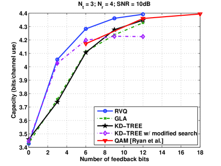
Figure 1: Shown is the ergodic capacity of the quantized beamforming vector for MIMO channel with 3 transmit and 4 receive antennas. The performance of different quantization schemes are shown with $B$ feedback bits.

In addition to channel capacity, we also examine the computational complexity of each quantization scheme required to search for the selected entry in the codebook. Fig. 2 shows the average number of matrix inner product computations used for each scheme versus the capacity with the same set of parameters as the previous figure. As expected, the RVQ codebook with a full search requires the most number of inner product computations, which grows exponentially as $B$ increases. At a capacity of 4.2 bits per channel use, the kd-tree requires almost two orders of magnitude less computations than RVQ does while the kd-tree with the modified search requires almost one order of magnitude less. The QAM codebook is the least complex for a large capacity, however it is not available for a low capacity.

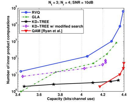
Figure 2: The average number of matrix inner product computations required to locate the selected entry for various quantization codebooks is shown with the ergodic capacity for MIMO channel with $N_{t}=3$, $N_{r}=4$, and $\rho=10\ \text{dB}$.

We compare the large system capacity approximation in Theorem 1 with the capacity of a finite-size MIMO channel with $N_{r}/N_{t}=1$ and show the comparison in Fig. 3. We note that there is a substantial gap between the theoretical approximation and the simulation results especially for the $2\times 2$ system. The gap narrows as the system size increases to $4\times 4$ and is expected to narrow further as the size increases. For the $2\times 2$ channel, one feedback bit per transmit antenna does not improve the capacity by much. However, as the system size increases, one feedback bit per antenna could potentially increase the capacity as much as 50% from the zero-feedback capacity.

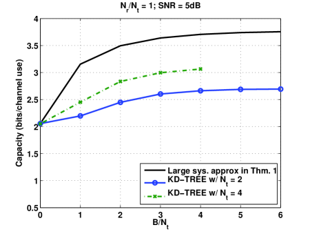
Figure 3: The asymptotic capacity approximation is shown with the capacity of $2\times 2$ and $4\times 4$ channels.

The simulation results for CDMA are shown in Fig. 4. The kd-tree codebook with a modified search has performance that is close to that of the RVQ codebook while the eigenvector-quantized schemes perform much worse, especially for small $\bar{B}$. We also plot the large system approximation in Theorem 2. Unlike the MIMO results, the derived approximation predicts the performance of the finite-size CDMA quite well since the system size here ($N=10$) is much larger than that in MIMO. We note that results for the RVQ codebook with large $\bar{B}$ are missing due to the very large memory requirement to store the codebook and the large computing power required to locate the codebook entry. In the case of the GLA and the kd-tree codebooks, the results for large $B$ are also missing because building a tree with large number of entries also demands very high computing power.

We also show the large system performance of the RVQ codebook derived in [21]. We remark that with one feedback bit per processing gain, SINR for the RVQ codebook is about 4 dB higher than that for the eigenvector-quantized codebooks. However, this advantage comes with a much larger search complexity as we will see in Fig. 5.

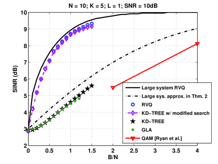
Figure 4: SINR with quantized signatures from different quantization schemes are compared.

Besides capacity, we would like to compare the complexity of each scheme to locate the selected entry from the RVQ codebook. The computational complexity will be measured by the number of inner products between two $N$-dimensional vectors. For an exhaustive search, the number of inner-product computations increases exponentially with $B$. For the proposed binary tree with the nearest-neighbor search, the number of inner-product computations depends on the tree’s depth and only increases linearly with $B$. The complexity of the kd-tree search is even less since in each search step, only one dimension of an $N$-dimensional codebook entry is required. Thus, the search complexity of the kd-tree is proportional to $B/N$. This also applies to the modified kd-tree search as well.

We compare the search complexity associated with different codebooks whose SINR performance is shown in Fig. 5. Similar to the results for the MIMO channel, the average number of inner product computations used to search the selected entry is shown. The RVQ codebook is the most complex while the kd-tree and QAM codebooks are the least complex. At 9 dB, the kd-tree codebook with a modified search requires about 3 orders of magnitude in search complexity less than RVQ does. The QAM codebook also requires few computations, however, it is not valid for small number of feedback bits.

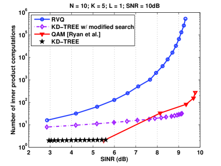
Figure 5: The average number of inner product computations to search for selected entry in the codebook for each quantization scheme is shown with SINR in dB.

VI Conclusions

We have proposed tree-structured RVQ codebooks to quantize the transmitted signature for CDMA and the beamforming vector for the MIMO channel. The tree structure is generated by either the GLA or kd-tree algorithms. For small-to-moderate feedback, the kd-tree codebook with a modified search has performance that is close to that of the RVQ with the exhaustive search. Thus, our proposed scheme complements the QAM codebook proposed by Ryan et al [9], which does not perform well in a low-feedback regime. For large feedback, quantizing the eigenvector with the GLA or the kd-tree codebooks produces a performance that is close to RVQ. The search complexity of the proposed schemes are a few orders of magnitude less than that of RVQ for a given performance. We also approximated the performance with large system limit, and numerical examples have shown that the approximations can predict the simulation results well for a moderate-size system.

In this study, we only consider quantization of a rank-one transmit beamforming vector in MIMO channels and single-user signature quantization in CDMA. To extend the existing results to MIMO channels with an arbitrary-rank precoding matrix or uplink CDMA with multiple-signature quantization, we can vectorize the precoding matrix or multiple signatures and apply the GLA or kd-tree algorithms to construct a tree. However, the mentioned scheme can be highly suboptimal. Thus, improving the scheme and analyzing the associated performance are interesting open problems.

References

- [1] D. J. Love, R. W. Heath, Jr., W. Santipach, and M. L. Honig, “What is the value of limited feedback for MIMO channels?” IEEE Commun. Mag., vol. 42, no. 10, pp. 54–59, Oct. 2004.
- [2] A. Narula, M. J. Lopez, M. D. Trott, and G. W. Wornell, “Efficient use of side information in multiple antenna data transmission over fading channels,” IEEE J. Sel. Areas Commun., vol. 16, no. 8, pp. 1423–1436, Oct. 1998.
- [3] D. J. Love and R. W. Heath, Jr., “Grassmannian beamforming for multiple-input multiple-output wireless systems,” IEEE Trans. Inf. Theory, vol. 49, no. 10, pp. 2735–2745, Oct. 2003.
- [4] K. K. Mukkavilli, A. Sabharwal, E. Erkip, and B. Aazhang, “On beamforming with finite rate feedback in multiple antenna systems,” IEEE Trans. Inf. Theory, vol. 49, no. 10, pp. 2562–2579, Oct. 2003.
- [5] J. C. Roh and B. D. Rao, “Transmit beamforming in multiple-antenna systems with finite rate feedback: A VQ-based approach,” IEEE Trans. Inf. Theory, vol. 52, no. 3, pp. 1101–1112, Mar. 2006.
- [6] W. Santipach and M. L. Honig, “Capacity of a multiple-antenna fading channel with a quantized precoding matrix,” IEEE Trans. Inf. Theory, vol. 55, no. 3, pp. 1218–1234, Mar. 2009.
- [7] ——, “Signature optimization for CDMA with limited feedback,” IEEE Trans. Inf. Theory, vol. 51, no. 10, pp. 3475–3492, Oct. 2005.
- [8] W. Dai, Y. Lui, and B. Rider, “Performance analysis of cdma siganture optimization with finite rate feedback,” in Proc. Conf. on Inform. Sciences ans Systems (CISS), Princeton, NJ, Mar. 2006.
- [9] D. J. Ryan, I. Clarkson, I. B. Collings, D. Guo, and M. L. Honig, “QAM and PSK codebooks for limited feedback MIMO beamforming,” IEEE Trans. Commun., vol. 57, no. 4, pp. 1184 –1196, Apr. 2009.
- [10] R. G. McKilliam, D. J. Ryan, I. V. L. Clarkson, and I. B. Collings, “An improved algorithm for optimal noncoherent QAM detection,” in Proc. Australian Commun. Theory Workshop, Christchurch, New Zealand, Jan. 2008, pp. 64–68.
- [11] D. J. Ryan, I. B. Collings, and I. V. L. Clarkson, “GLRT-optimal noncoherent lattice decoding,” IEEE Trans. Signal Process., vol. 55, no. 7, pp. 3773–3786, Jul. 2007.
- [12] J. Max, “Quantizing for minimum distortion,” IEEE Trans. Inf. Theory, vol. 6, pp. 7–12, Mar. 1960.
- [13] S. P. Lloyd, “Least squares quantization in PCM,” IEEE Trans. Inf. Theory, vol. 28, no. 2, pp. 129–137, Mar. 1982.
- [14] J. L. Bentley, “Multidimisional divide and conquer,” Communications of the ACM, vol. 22, no. 4, pp. 214–229, 1980.
- [15] ——, “K-d trees for semidynamic point sets,” in Proc. the Sixth Annual Symposium on Computational Geometry, Berkeley, California, 1990, pp. 187 – 197.
- [16] K. Mamat and W. Santipach, “Multiuser signature quantization with tree-structured codebook in DS-CDMA,” in Proc. ECTI-CON, vol. 2, Pattaya, Thailand, May 2009, pp. 870–873.
- [17] A. Gersho and R. M. Gray, Vector Quantization and Signal Compression. Springer, 1991.
- [18] I. Katsavounidis, C.-C. J. Kuo, and Z. Zhang, “Fast tree-structured nearest neighbor encoding for vector quantization,” IEEE Trans. Image Process., vol. 5, no. 2, pp. 398–404, Feb. 1996.
- [19] A. M. Tulino and S. Verdú, “Random matrix theory and wireless communications,” Foundations and Trends in Communications and Information Theory, vol. 1, no. 1, pp. 1–182, 2004.
- [20] W. Santipach, “Signature quantization in fading CDMA with limited feedback,” IEEE Trans. Commun., vol. 59, no. 2, pp. 569–577, Feb. 2011.
- [21] W. Dai, Y. Liu, and B. Rider, “The effect of finite rate feedback on CDMA signature optimization and MIMO beamforming vector selection,” IEEE Trans. Inf. Theory, vol. 55, no. 8, pp. 3651–3669, Aug. 2009.