Nuclear Dynamics During Landau-Zener Singlet-Triplet Transitions in Double Quantum Dots

Abstract

We consider nuclear spin dynamics in a two-electron double dot system near the intersection of the electron spin singlet $S$ and the lower energy component $T_{+}$ of the spin triplet. The electron spin interacts with nuclear spins and is influenced by the spin-orbit coupling. Our approach is based on a quantum description of the electron spin in combination with the coherent semiclassical dynamics of nuclear spins. We consider single and double Landau-Zener passages across the $S$-$T_{+}$ anticrossings. For linear sweeps, the electron dynamics is expressed in terms of parabolic cylinder functions. The dynamical nuclear polarization is described by two complex conjugate functions $\Lambda^{\pm}$ related to the integrals of the products of the singlet and triplet amplitudes ${\tilde{c}}_{S}^{\ast}{\tilde{c}}_{T_{+}}$ along the sweep. The real part $P$ of $\Lambda^{\pm}$ is related to the $S$-$T_{+}$ spin-transition probability, accumulates in the vicinity of the anticrossing, and for long linear passages coincides with the Landau-Zener probability $P_{LZ}=1-e^{-2\pi\gamma}$, where $\gamma$ is the Landau-Zener parameter. The imaginary part $Q$ of $\Lambda^{+}$ is specific for the nuclear spin dynamics, accumulates during the whole sweep, and for $\gamma\gtrsim 1$ is typically an order of magnitude larger than $P$. $P$ and $Q$ also show critically different dependences on the shape and the duration of the sweep. $Q$ has a profound effect on the nuclear spin dynamics, by (i) causing intensive shake-up processes among the nuclear spins and (ii) producing a high nuclear spin generation rate when the hyperfine and spin-orbit interactions are comparable in magnitude. Even in the absence of spin-orbit coupling, when the change in the the total angular momentum of nuclear spins is less than $\hbar$ per single Landau-Zener passage, the change in the global nuclear configuration might be considerably larger due to the nuclear spin shake-ups. We find analytical expressions for the back-action of the nuclear reservoir represented via the change in the Overhauser fields the electron subsystem experiences.

I Introduction

Electron spin states in semiconductor quantum dots are investigated for their potential use as quantum bits in quantum computing architectures.Hanson:rmp07 ; Loss:prb98 ; Levy:prl02 To this end, control of the spin states and their couplings to the environment is essential. In GaAs and InAs semiconductors, a major source of electron spin decoherence is the coupling to the surrounding nuclear spins.Merkulov:prb02 ; Khaetskii:prb03 ; Erlingsson:prb04 ; Hanson:rmp07 ; LuSham ; Cywinski Since the quantum dots are large compared to the interatomic spacing, each electron interacts with typically one million nuclei. Achieving control over this many-body interaction is a key for manipulating semiconductor quantum bits.

In two electron double quantum dots, the singlet $S$ and triplet $T_{0}$ states define the elementary qubit. The coupling between these states is governed by the gradient in the longitudinal magnetic Zeeman splitting between the two dots. Controlling this coupling enables singlet-triplet qubit manipulations. Beyond the two-state $S$-$T_{0}$ qubit operation, the gradient in the transverse magnetic Zeeman splitting between the two dots defines the coupling of the singlet $S$ to the triplet $T_{+}$ and $T_{-}$ states. Finally, the longitudinal magnetic Zeeman splitting determines the relative energies of the triplet states. This Zeeman splitting arises from the external field $\mathbf{B}$ and the nuclear spin background via the Overhauser field, and by changing the nuclear spin polarization the basic electron parameters can be tuned.

Polarization of nuclear spins can be created and destroyed by flip-flop processes by pumping the electronic states via time-dependent gate voltages. This has recently been investigated in many interesting experimentalBarthel ; Foletti:nphys09 ; Bluhm:prl10 ; Bluhm:nphys11 and theoretical papers in double quantum dots in the regime of Pauli blockade.Ramon:prb07 ; Gullans:prl10 ; Stopa:prb10 ; Rudner:prb10a ; Rudner:prb10b Experimentally, it has been demonstrated that an Overhauser field gradient of several hundred milli Tesla can be generated and sustained.Foletti:nphys09 The dephasing time of the electron-spin qubits has been extended to more than 200 $\mu s$.Bluhm:nphys11 Because the dynamical interaction of an electron spin with a nuclear spin reservoir is enormously complicated, different theoretical efforts were focused on the various aspects of it. The two aspects most closely related to our paper are the theoretical modeling of the connection between the generation of dynamical nuclear spin polarization at short and long time scalesRamon:prb07 ; Gullans:prl10 ; Burkard and the influence of the spin-orbit interaction on the build-up of the nuclear polarization.Rudner:prb10a ; Rudner:prb10b

The aim of this paper is to study in detail the electron and nuclear spin dynamics as the system passes across a $S$-$T_{+}$ anticrossing. In GaAs and InAs quantum dots in an external magnetic field, $T_{+}$ is the lowest energy component of the electron triplet state because of the negative electron $g$-factor, $g<0$. During a $S$-$T_{+}$ (or a $T_{+}$-$S$) passage, electrons trade their spin with the nuclear reservoir, and multiple passages are used in creating a difference (”gradient”) of the effective nuclear (Overhauser) fields between two parts of the double dot that are used for qubit rotations. The study of a single passage (or two passages during a single cycle) provides a firm basis for investigating events on longer time scales. Also, the progress in experimental techniques currently allows, instead of averaging data over thousands of sweeps, to perform single-shot measurements,SingleShot and most recently such measurements have been achieved for double quantum dots.Barthel Also, the double dot dynamics during a single sweep manifests itself explicitly in beam splitter experiments.Petta2010 We expect the approach developed in our paper to become a useful tool in discussing such types of experiments and, more widely, to facilitate better understanding and utilization of the nuclear spin environment in solid state based quantum computing.

Specifically, we take into account the spatial distribution of the hyperfine coupling between the electron and nuclear spins and compute the change in the topography of the nuclear spin polarization and the related changes in the gradient and average Overhauser fields governing the dynamics of the electron spin. These fields, that the electrons experience in the singlet and triplet states, depend on the spatial variation of the electron-nuclear coupling and we take this dependence into account. We employ the Zener approachZener:prs32 and find analytically explicit expressions for the electron and nuclear spin dynamics during a single linear sweep and during cycles consisting of two linear sweeps.

Let us give an overview of the main results. We express the whole electron and nuclear spin dynamics in terms of two complex conjugate functions $\Lambda^{\pm}(T_{i},T_{f})$ depending on the initial and finite times $(T_{i},T_{f})$ and the shape of the path between them. These $\Lambda^{\pm}$ functions are integrals of the products of the singlet and triplet amplitudes during the $S$-$T_{+}$ passage. The real part $P=\text{Re}\{\Lambda^{\pm}\}$ is the transition probability between the singlet $S$ and the triplet $T_{+}$ states. The imaginary part $Q=\text{Im}\{\Lambda^{+}\}$ includes basic information about the nuclear spin dynamics including the nuclear shake-ups. The Landau-Zener probability, $P_{LZ}=1-e^{-2\pi\gamma}$, where $\gamma$ is the Landau-Zener parameter, is the asymptotic value of $P(T_{i},T_{f})$ for a single sweep when $T_{i}\rightarrow-\infty$ and $T_{f}\rightarrow\infty$. Usually, all results are expressed in terms of $P_{LZ}$. Our approach provides a more detailed information about the nuclear spin dynamics away from the $S-T_{+}$ anticrossing.

Oscillations of the transition probability $P(T_{i},T_{f})$ as a function of its arguments reveal typical interference patterns. These oscillations are highly anharmonic for small Landau-Zener transition probabilities $P_{LZ}\ll 1$ and might persist for a long time with a large amplitude for intermediate Landau-Zener transition probabilities $P_{LZ}\sim 0.5$. However, it is not typically the transition probability $P$ that determines the nuclear spin dynamics. Instead, the other $S$-$T_{+}$ quantity, $Q$ is non less important. While $P$ is constrained to be in the interval $0\leq P\leq 1$, there are no such constraints on $Q$ and it is typically larger than $P$. We find that $Q$ controls the shake-up processes among the nuclear spins. In the absence of spin-orbit coupling, at most $\hbar$ of the angular momentum can be transferred to the nuclear spin bath. Given that there are around a million nuclear spins in the quantum dots, of which around a thousand are aligned initially, a change in one out of a thousand nuclear spins would have only a minor effect. However, the nuclear spins are allowed to interchange their spins during the $S$-$T_{+}$ passage without violating the conservation of the angular momentum. Although the interchange does not change the total nuclear spin angular momentum, the redistribution of the nuclear spins can lead to considerable changes in the various gradient and average Overhauser fields that the electrons experience. This is because the Overhauser fields depend on weighted average values of the nuclear spin distribution with respect to the electron-nuclear couplings and not just the total nuclear spin. We find that such shake-ups are very sensitive to the initial nuclear spin distribution and that they are often much larger than the average nuclear spin production because $Q$ is typically ten times larger than $P$.

Furthermore, when the spin-orbit coupling competes with the hyperfine interaction and $Q$ is considerably larger than $P$, then the $Q$-enhanced spin generation dominates for a generic direction of the nuclear spin polarization and can become considerably larger than $P$. However, after averaging over the direction of the transverse nuclear spin polarization, $Q$ cancels and the results of Refs. [Rudner:prb10a, ; Rudner:prb10b, ] are recovered.

Another finding is that even geometrically symmetric double quantum dots acquire asymmetric behavior because of the spatial inhomogeneity of the hyperfine coupling. The sign of the asymmetry depends on $B$, and its magnitude is largest close to the (0,2) or (2,0) configuration. The consequences of this $B$-controlled asymmetry for building nuclear field gradients are similar to that envisioned in Ref. Gullans:prl10, for geometrically asymmetric dots.

This paper is organized in the following way. In Sec. II, we describe the model of a double quantum dot that follows the lines of Refs. [Taylor:nphys05, ; Taylor:prb07, ; Gullans:prl10, ]. We introduce the basic notations related to the electron-nuclear hyperfine interaction and the nuclear dynamics induced by it in Secs. III and IV, respectively. In Sec. V, a linear Landau-Zener sweep is treated analytically and the time-dependence of the effective magnetic fields acting on the nuclei is discussed in detail. Because Sec. V is rather technical, a reader interested in experimental applications can skip to Sec. VI, where numerical data for the linear in time Landau-Zener sweeps and cycles are discussed. In Sec. VII, the back action of the nuclear spin dynamics on the Overhauser fields in the electron spin Hamiltonian is estimated. Appendix A outlines the notations for electron spin operators. Appendix B discusses the spatial dependence of the hyperfine interaction. We demonstrate that even for two symmetric quantum dots, the hyperfine coupling acquires asymmetries controlled by the overlap integral and the external magnetic field. Appendix C includes two new identities for parabolic cylinder functions. We conclude and summarize our results in Sec. VIII.

II Model

We consider two electrons in a double quantum dot. When the electron spin is conserved, the classification of the electron states as a singlet state $S$ and three triplet ($T_{\nu}$, $\nu=0,\pm 1$) states is exact. Spin-orbit interaction and the interaction with the nuclear spins mixes these states. We use the singlet and triplet stationary states as our basis. They are

$$\Psi_{S}(1,2) =\psi_{S}(1,2)\chi_{S}(1,2)\,,$$ (1a)

$$\Psi_{T_{\nu}}(1,2) =\psi_{T}(1,2)\chi_{T_{\nu}}(1,2)\,,$$ (1b)

where 1 and 2 denote the 1st and 2nd electron. The spin wave functions obey the symmetries $$\chi_{S}(1,2)=-\chi_{S}(2,1) \chi_{T_{\nu}}(1,2)=\chi_{T_{\nu}}(2,1) \psi_{S}(1,2) \psi_{T}(1,2) \psi_{S}(1,2)=\psi_{S}(2,1) \,\,\psi_{T}(1,2)=-\psi_{T}(2,1),$$ as well as and are specified in Appendix B. The orbital wave functions and obey the symmetries and and we consider only the lowest energy orbital states so there are no additional quantum numbers labeling the orbital wave functions.

The electrons interact with each other, external gate potentials, an external magnetic field, and with the nuclear spins predominantly via the hyperfine interaction. The latter interaction, as well as spin-orbit coupling, induce transitions between the singlet and triplet states that we compute. The nuclei interact with the external magnetic field, the electrons through the hyperfine interaction, and with each other via the magnetic dipole-dipole interaction. The latter interaction affects the nuclear spin dynamics on long time scales of around milli seconds, and we disregard it in what follows. However, we take into account (in a semiclassical Born-Oppenheimer approach and in the leading order in the large electron Zeeman splitting) an indirect RKKY-like interaction between nuclear spins originating from the hyperfine electron-nuclear coupling (see Sec.  V.4). Near the $ST_{+}$ anticrossing it manifests itself at the scale of about 10 $\mu$s.

Of central importance is the hyperfine electron-nuclear interaction

$$\hat{H}_{hf}=A\sum_{j}\sum_{\ell=1}^{2}\delta(\mathbf{{R}_{j}-r_{\ell})(\hat{I}_{j}\cdot\hat{\mathbf{s}}(\ell)),}$$ (2)

where $A$ is the electron-nuclear interaction strength, $\ell$ numerates electrons and $j$ nuclei, $\hat{\mathbf{s}}(\ell)=\frac{1}{2}\hat{\bm{\sigma}}(\ell)$ are the electron spin operators in terms of the vector of Pauli matrices $\hat{\bm{\sigma}}(\ell)$ for each electron $\ell$, and $\hat{\mathbf{I_{j}}}$ are the nuclear spin operators. The electron and nuclear spin operators are dimensionless in our notations. Carets denote quantum mechanical operators and bold variables are vectors.

In the $4\times 4$ singlet and triplet space ($S,T_{+},T_{0}$, and $T_{-}$), the Hamiltonian that describes the electrons and their interaction with the nuclear spins can be written as

$${\hat{H}}=\left(\begin{array}[]{cc}\epsilon_{S}&\mathbf{\hat{v}}_{n}^{T}\\ \mathbf{\hat{v}}_{n}^{\ast}&\epsilon_{T}-\mathbf{\hat{\eta}\cdot\hat{S}}\end{array}\right),$$ (3)

where the total electron spin ${\hat{\mathbf{S}}}=\hat{\mathbf{s}}(1)+\hat{\mathbf{s}}(2)$. Additionally, the spin-orbit interaction induces terms in Eq. (3) that we discuss below. The nuclear spins are also affected by the external magnetic field through the nuclear Zeeman effect that we take into account below in the description of their dynamics. However, we disregard the effect of the nuclear Zeeman energy on the equilibrium spin populations because of the high temperature of the nuclear spin bath. The $\epsilon_{S}$ and $\epsilon_{T}$ terms in the diagonal matrix elements of Eq. (3) describe the singlet and triplet energies in the absence of the nuclear and external magnetic fields. They depend on the electrostatic gate potentials and the interactions between the electrons. The off-diagonal operator components $\mathbf{\hat{v}}_{n}^{T}=(\hat{v}_{n}^{+},-\hat{v}_{n}^{z},-\hat{v}_{n}^{-}),$ are nuclear spin dependent (a superscript $T$ denotes the transpose of a vector and the subscript $n$ denotes that this coupling is due to the nuclear spins)

$$\hat{v}_{n}^{\alpha}=A\sum_{j}\rho_{j}\hat{I}_{j}^{\alpha},$$ (4)

with $\alpha=(+$, $-$, $z)$, $\hat{I}_{j}^{\pm}=\left(\hat{I}_{j}^{x}\pm i\hat{I}_{j}^{y}\right)/\sqrt{2}$ are the transverse nuclear spin components, and the singlet-triplet electron-nuclear coupling coefficients

$$\rho_{j}=\rho(\mathbf{R}_{j})=\int d\mathbf{r}\psi_{S}^{\ast}(\mathbf{r},\mathbf{R}_{j})\psi_{T}(\mathbf{r},\mathbf{R}_{j})$$ (5)

dependent on the positions $\mathbf{R}_{j}$ of nuclei $j$. Roughly, $\rho_{j}$ varies from positive in one quantum dot to negative in the other. Therefore, $\hat{v}_{n}^{\pm}$ and $\hat{v}_{n}^{z}$ represent differences in the effective nuclear magnetic fields in the two dots in the directions transverse and parallel to the external magnetic field, respectively. The effective splitting of the triplet states due to the external magnetic field $\mathbf{B}$ and the nuclei is $-\mathbf{\hat{\eta}\cdot\hat{S}}$, where

$$\mathbf{\hat{\eta}}=\eta_{Z}\mathbf{e}_{z}\,+\mathbf{\hat{\eta}}_{n}=\eta_{Z}\mathbf{e}_{z}\,-A\sum_{j}\zeta_{j}\mathbf{\hat{I}}_{j}\,,$$ (6)

$\eta_{Z}$ is the electron Zeeman splitting in the field $\mathbf{B}\parallel{\hat{\mathbf{z}}}$, $\mathbf{\hat{S}}$ is the spin-1 operator for the electrons (as defined in Appendix A), and the position dependent coupling constants of the triplet states to the nuclei are

$$\zeta_{j}=\int d\mathbf{r}\psi_{T}^{\ast}(\mathbf{r},\mathbf{R}_{j})\psi_{T}(\mathbf{r},\mathbf{R}_{j}).$$ (7)

This completes the description of the Hamiltonian that governs the coupling between the electron and nuclear spin dynamics.

The $ST_{+}$ anticrossings arising due to $\hat{v}_{n}^{\alpha}$ and also the $ST_{0}$ level splittings were investigated by the beam-splitting techniquePetta2010 and Rabi-oscillations Petta2005 ; Foletti:nphys09 ; Bluhm:prl10 , respectively.

III Electron and nuclear spin dynamics

The Hamiltonian of Eq. (3) defines a many-body problem of the coupled electron-nuclear dynamics. Our interest is in the dynamical nuclear polarization that is achieved by changing the gate voltages in such a way that the electronic subsystem makes a transition from the singlet $S$ to the lowest energy triplet $T_{+}$ state or vice versa. The many-body interaction can be simplified by employing the Born-Oppenheimer approach.Gullans:prl10 The electrons are fast as compared to the nuclei. The electrons also interact with a large number of nuclei, around one million. These two features imply that the electron dynamics is unaffected by the dynamics of a single nucleus and electrons see only a quasi-static configuration of all nuclei during a single $ST_{+}$ crossing. This motivates an ansatz where the wave function is separable into electronic and nuclei parts.Gullans:prl10

The electron dynamics can be solved from the Hamiltonian of Eq. (3) with the assumption that the nuclear spin operators can be approximated by their expectation values before the transition, $\mathbf{\hat{v}}_{n}\rightarrow\mathbf{v}_{n}$. The detuning energy $\epsilon$ is defined as the difference between the triplet energy $\epsilon_{T_{0}}$ and the singlet energy $\epsilon_{S}$, $\epsilon=\epsilon_{T_{0}}-\epsilon_{S}$, and is controlled by the variations in the gate voltages. We restrict ourselves to the limit of a rather large external magnetic field so that the splitting between the triplet states is larger than the magnitude of the off-diagonal matrix elements that mix the singlet and triplet states. When the separation between the energy levels is much larger than the matrix elements that mix the singlet and triplet states, the singlet and triplet states are well separated. The singlet-triplet matrix elements produce anti-crossings between the singlet and triplet levels when their energies are tuned to be close to resonance. Our focus is on situations where the system is tuned close to the $S$-$T_{+}$ transition as shown in Fig. 1

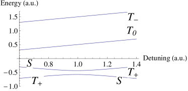
Figure 1: Schematics of the singlet and triplet energy levels as a function of the detuning energy $\epsilon=\epsilon_{T_{0}}-\epsilon_{S}$ close to the $S$-$T_{+}$ anticrossing. The Zeeman splitting $\eta_{Z}=1$ is chosen as the energy unit, off-diagonal matrix elements are $v^{\perp}=|v^{\pm}|=0.07$.

There, the energies of the triplet states $T_{0}$ and $T_{-}$ are of the order the electron Zeeman splitting $\eta^{z}$ away from the energies of singlet $S$ and triplet $T_{+}$ states, which is a large energy as compared to the $S$-$T_{+}$ anticrossing width. In this case, the electron dynamics can be approximated by the $2\times 2$ dynamics for the singlet $S$ and triplet $T_{+}$ amplitudes of the electron wave function. The reduction of the original $4\times 4$ electron dynamics problem to a $2\times 2$ problem also facilitates finding an exact solution for the electron dynamics for linear sweeps and allows to reveal the role of the long time “tails” of the singlet and triplet amplitudes crucial for the nuclear spin dynamics. In the $2\times 2$ basis, the electron dynamics is described by the singlet $c_{S}$ and triplet $c_{T_{+}}$ amplitudes that obey a Schrödinger equation

$$H^{(ST_{+})}\left(\begin{array}[]{c}c_{S}\\ c_{T_{+}}\end{array}\right)=i\hbar\partial_{t}\left(\begin{array}[]{c}c_{S}\\ c_{T_{+}}\end{array}\right)$$ (8)

with the Hamiltonian

$$H^{(ST_{+})}=\left(\begin{array}[]{cc}\epsilon_{S}&v^{+}\\ v^{-}&\epsilon_{T_{+}}\end{array}\right),$$ (9)

where $\epsilon_{T_{+}}=\epsilon_{T}-\eta^{z}$, and following Refs. [Rudner:prb10a, ; Rudner:prb10b, ] we have included the spin-orbit matrix elements $v_{so}^{\pm}$ that couple $S$ and $T_{+}$ states into the total off-diagonal matrix elements

$$v^{\pm}=v_{n}^{\pm}+v_{so}^{\pm}.$$ (10)

While the coupling between $S$ and $T$ levels in GaAs double quantum dots is usually attributed to the hyperfine interaction, spin-orbit coupling is inevitably present while difficult to evaluate quantitively for specific devices.Novak2011 It manifests itself in spin relaxation,KhaetskiiNazarov ; BulaevLoss level anticrossings in InAs single and double dots,Takahashi ; Pfund2007 and in the EDSREDSR ; Golovach both in GaAsNowack07 ; Tarucha08 and InAsNadjPerge double dots. It is important to emphasize the existence of different mechanisms that couple the electron spin to the orbital degrees of freedom. They include the traditional (Thomas) spin-orbit interaction that couples the electron spin to the electron momentum and the Zeeman interaction in a inhomogeneous magnetic field $\mathbf{B}(\mathbf{r})$ that couples the electron spin to the elecron coordinate.Rashba05 In Ref. Nowack07, , the first mechanism dominated while in Refs. Laird07, and Tarucha08, different versions of the second one were important. We show in what follows that spin-orbit coupling also has a profound effect on the nuclear spin polarization production rate.

By carrying out a unitary transformation of the original $4\times 4$ Hamiltonian, it can be shown that the corrections to the reduced $2\times 2$ Hamiltonian of Eq. (9) are quadratic in the small ratio between $v^{\pm}$ and the Zeeman splitting $\eta_{Z}$ provided the gate-voltage induced $S$-$T_{+}$ transition is slow so that $\hbar(\dot{\epsilon}_{S}-\dot{\epsilon}_{T})/\eta_{Z}^{2}\ll 1$. We assume that this criterion is satisfied.

In turn, the dynamics of nuclear spins is driven by the effective magnetic fields $\bm{\Delta}_{j}$ arising from the electron dynamics

$$\hbar\frac{d\mathbf{\hat{I}}_{j}}{dt}=\bm{\Delta}_{j}\times\mathbf{\hat{I}}_{j},$$ (11)

where the components of the fields $\bm{\Delta}_{j}$ acting on the nuclei are the transverse $\Delta_{j}^{\pm}=\left(\Delta_{j}^{x}\pm i\Delta_{j}^{y}\right)/\sqrt{2}$ and longitudinal $\Delta_{j}^{z}$ fields:

$$\Delta_{j}^{+} =A\rho_{j}c_{S}c_{T_{+}}^{\ast},$$ (12a)

$$\Delta_{j}^{-} =A\rho_{j}c_{S}^{\ast}c_{T_{+}},$$ (12b)

$$\Delta_{j}^{z} =A\zeta_{j}|c_{T_{+}}|^{2}-\eta_{j(nZ)},$$ (12c)

and $$\eta_{j(nZ)} j (c_{S}(t),c_{T_{+}}(t)) v^{\pm} \bm{\Delta}_{j}$$ is the nuclear Zeeman splitting for the nucleus . Because the dynamics of electron amplitudes depends not only on the potentials on the gates but also on the nuclear spins through the matrix elements , fields can be considered as dynamical RKKY fields.

In the next section we show how the changes in the electronic states as they pass across the $S$-$T_{+}$ anticrossing change the spatially dependent nuclear polarization.

IV Dynamical Nuclear Polarization

We consider a situation where the changes in the gate voltages can induce a singlet $S$ to triplet $T_{+}$ transition or vice versa, so that the total electron angular momentum may be increased or reduced by 1. In the absence of spin-orbit coupling, this implies that the change in the $z$-projection of the total nuclear spin equals the change in the elecron spin (but with the opposite sign). There is no conservation law for the spatial distribution of the nuclear spin. We are interested in how this change of angular momentum is distributed among the nuclei. As already mentioned above, the typical time scale for nuclei dynamics is long as compared to the time scale for the electron dynamics, in particular, with the singlet-triplet transition time. Let us denote the initial time of the sweep as $T_{i}$ and the final time as $T_{f}$. We assume that the duration of the Landau-Zener sweep, $T_{f}-T_{i}$, is short as compared to the typical nuclear spin precession time and take the nuclear dynamics into account as a perturbation. Also, since the total change of the angular momentum is of the order $1$, the typical change in the individual nuclear spins is much less than $1$. With these assumptions, the change of a nuclear spin $\Delta\mathbf{\hat{I}}_{j}=\mathbf{\hat{I}}_{j}(T_{f})-\mathbf{\hat{I}}_{j}(T_{i})$ during a Landau-Zener transition is

$$\Delta\mathbf{\hat{I}}_{j}=\bm{\Gamma}_{j}(T_{f},T_{i})\times\mathbf{\hat{I}}_{j}(T_{i}),$$ (13)

where the total effect of the electrons on the nuclei is the integrated effect of the magnetic splitting in Eqs. (12a), (12b), and (12c) :

$$\bm{\Gamma}_{j}(T_{f},T_{i})=\int_{T_{i}}^{T_{f}}\frac{dt}{\hbar}\bm{\Delta}_{j}(t).$$ (14)

In order to find explicit expressions for the dependence of the electron states on the effective field induced by the transverse nuclear spin polarization $v_{n}^{\pm}$, it is convenient to make a transformation of the singlet and triplet amplitudes

$$c_{s}=\tilde{c}_{s}\text{, \ \ }c_{T_{+}}=\tilde{c}_{T_{+}}v^{-}/v_{\bot}.$$ (15)

Then the Hamiltonian becomes real, and

$$\left(\begin{array}[]{cc}\epsilon_{s}&v_{\bot}\\ v_{\bot}&\epsilon_{T_{+}}\end{array}\right)\left(\begin{array}[]{c}\tilde{c}_{S}\\ \tilde{c}_{T_{+}}\end{array}\right)=i\hbar\partial_{t}\left(\begin{array}[]{c}\tilde{c}_{S}\\ \tilde{c}_{T_{+}}\end{array}\right),$$ (16)

where $v_{\bot}=\left|v^{\pm}\right|$. Eq. (16) depends, in addition to the external magnetic field, on the absolute value of the combined effect of the nuclear spin induced transverse effective field and spin-orbit interaction, but does not depend on its direction.

In this basis, we can express the total effect of the $(x,y)$ components of the effective field of Eq. (14) in terms of

$$\Gamma_{j}^{\pm}=\pm iA\rho_{j}\Lambda^{\pm}v^{\pm}/(2v_{\bot}^{2})\,,$$ (17)

where the dimensionless functions $\Lambda^{\pm}(T_{i},T_{f})$ are defined as

$$\Lambda^{-}=i2v_{\bot}\int_{T_{i}}^{T_{f}}\frac{dt}{\hbar}\tilde{c}_{S}^{\ast}(t)\tilde{c}_{T_{+}}(t),$$ (18)

and $\Lambda^{+}=\left(\Lambda^{-}\right)^{\ast}$. This expression can be transformed by using the equation $\tilde{c}_{T_{+}}=v_{\bot}^{-1}(i\hbar\partial_{t}-\epsilon_{s}(t))\tilde{c}_{s}$ following from Eq. (16),

$$\Lambda^{-}=-2\int_{T_{i}}^{T_{f}}dt\tilde{c}_{S}^{\ast}(t)\frac{\partial\tilde{c}_{s}(t)}{\partial t}-i2\int_{T_{i}}^{T_{f}}\frac{dt}{\hbar}\epsilon_{s}(t)\left|c_{s}(t)\right|^{2},$$ (19)

so that

$$\text{Re}\{\Lambda^{\pm}\}=P=\left|c_{s}(T_{i})\right|^{2}-\left|c_{s}(T_{f})\right|^{2},$$ (20)

is the transition probability $P(T_{i},T_{f})$ from the singlet $S$ to the triplet $T_{+}$ state. There is no such a simple relation between the imaginary parts of $\Lambda^{\pm}$ and the transition probability, and this fact is important for the following discussion of the effect of the Landau-Zener sweeps on nuclei. However, we observe that when the Hamiltonian in the Schrödinger equation (16) is stationary, i.e., when the gate voltages are fixed and $\epsilon_{S}$ and $\epsilon_{T_{+}}$ are constant in time, and the system is in an eigenstate of the Hamiltonian of Eq. (16), the field $\tilde{c}_{S}^{\ast}\tilde{c}_{T_{+}}$ is real implying a nonvanishing imaginary contribution to $\Lambda^{\pm}$. The imaginary part of $\Lambda^{\pm}$ thus includes contributions that can be understood in terms of RKKY-like static nuclear spin-spin interaction mediated by the electronic state, but this interaction also depends on the spin-orbit coupling. We will diagonalize the stationary Hamiltonian of Eq. (16) in Sec. V.4 and relate the imaginary part of $\Lambda^{\pm}$ to the static electronic properties and show how this influences the dynamical nuclear dynamical properties. The imaginary part of $\Lambda^{\pm}$ is central for the understanding of the dynamical nuclear polarization and we define

$$Q=\text{Im}\{\Lambda^{+}\}=-\text{Im}\{\Lambda^{-}\}.$$ (21)

We also express the total effect of the field along $z$ as

$$\Gamma_{j}^{z}=A\zeta_{j}\Lambda^{z}/(2v_{\bot})-\eta_{j(nZ)}(T_{f}-T_{i})/\hbar,$$ (22)

where

$$\Lambda^{z}=2v_{\bot}\int_{T_{i}}^{T_{f}}\frac{dt}{\hbar}\left|\tilde{c}_{T_{+}}(t)\right|^{2}.$$ (23)

Using Eqs. (12a), (12b), and (12c), as well as expressing $\Gamma_{j}^{\pm}$ and $\Gamma_{j}^{z}$ of Eqs. (17) and (23) in terms of $\Lambda^{\pm}$ and $\Lambda^{z}$, we arrive at the spin production during a single $S\rightarrow T_{+}$ transition both in the transverse

$$\Delta\hat{I}_{j}^{\pm} = \frac{A}{2v_{\bot}}\left[\frac{v^{\pm}}{v_{\bot}}\Lambda^{\pm}\rho_{j}\hat{I}_{j}^{z}\pm i\Lambda^{z}\zeta_{j}\hat{I}_{j}^{\pm}\right]$$ (24)

$$\mp i\frac{\eta_{j(nZ)}}{\hbar}(T_{f}-T_{i})\hat{I}_{j}^{\pm}$$

and the longitudinal components

$$\Delta\hat{I}_{j}^{z}=-\frac{A}{2v_{\bot}^{2}}\left[\Lambda^{-}v^{-}\rho_{j}\hat{I}_{j}^{+}+\Lambda^{+}v^{+}\rho_{j}\hat{I}_{j}^{-}\right].$$ (25)

Next, substituting operators $\hat{v}_{n}^{\pm}$ in Eq. (4) by their semiclassical values $v_{n}^{\pm}$ and using Eq. (10), we find the change in the $z$-component of the total nuclear spin, $\Delta I^{z}=\sum\limits_{j}\Delta I_{j}^{z}$,

$$\Delta I^{z}=-P+\frac{1}{2v_{\bot}^{2}}\left[\Lambda^{-}v^{-}v_{so}^{+}+\Lambda^{+}v^{+}v_{so}^{-}\right],$$ (26)

or

$$\Delta I^{z}=-\frac{P}{2v^{2}_{\perp}}(v^{-}v_{n}^{+}+v^{+}v_{n}^{-})-i\frac{Q}{2v^{2}_{\perp}}(v^{-}v_{n}^{+}-v^{+}v_{n}^{-}).$$ (27)

Note that the change in the $z$-component of the total nuclear spin is computed under the constraint that the transverse nuclear fields are $v_{n}^{\pm}$ before the sweep.

Remarkably, $\Delta I^{z}$ of Eq. (26) only depends on the basic parameters of the Hamiltonian ${H}^{(ST_{+})}$ of Eq. (9) and the shape of the sweep and does not depend on the detailed topography of nuclear spins. Therefore, the result is very general and convenient to use. In this respect, transfer of the longitudinal component of the angular momentum differs from the transfer of its transverse component that, according to Eq. (24), depends on the specific spin configuration.

In the absence of spin-orbit interaction, $v_{so}^{\pm}=0$, the total change in the electron spin equals the transition probability $P$, as expected for a (partial) transition between the singlet $S$ and triplet $T_{+}$ states. Conservation of the $z$ component of the angular momentum then dictates that the change in the $z$ component of the total nuclear spin equals $-P$. Spin-orbit coupling breaks the conservation law for the angular momentum transfer from the electronic to the nuclear spin system since angular momentum can be transferred to or from the lattice as well. Such processes manifest themselves in the second term in Eq. (26). It depends on the relative phase between the spin-orbit and hyperfine interaction matrix elements. Furthermore, this term depends not only on the transition probability $P$, but also on the imaginary parts of $\Lambda^{\pm}$. $Q$ acquires contributions not only from the part of the sweep near the anticrossing point but also from its long tails. As a result, the magnitude of $Q$ can be much larger than $P$ for certain classes of sweeps. This generic feature suggests that $Q$ can be made large, and the spin-orbit coupling can strongly influence nuclear dynamics even when it is weaker than the hyperfine coupling.

Our results confirm the prediction of Ref. Rudner:prb10b, that the spin-orbit coupling influences the nuclear spin generation rate profoundly. The quantity computed in Ref. Rudner:prb10b, is the total change of the nuclear spin $\Delta I^{z}$ averaged over the phase of the transverse nuclear field $v_{n}^{\pm}$. This averaging annihilates the second term of Eq. (27) while the first term coincides with Eq. (9) in Ref. Rudner:prb10b, .RudnerProof Since $Q$ can be considerably larger than $P$, we expect enhancement of spin production rate in experiments performed at a fixed (while generic) values of $v_{n}^{\pm}$.

V Linear sweeps - Landau-Zener electron transitions

When the changes in the gate voltages are such that the difference in the energy betwen the singlet $S$ and the triplet $T_{+}$ varies linearly in time, Eq. (16) reduces to the standard Landau-Zener problem. Because the Landau approach based on analytical continuation allows finding only the transition probabilities,LL:book65 we employ in the following the Zener approachZener:prs32 allowing finding explicit expressions for the time dependence of electron wave functions that drives the coherent nuclear spin dynamics. We consider a transition from the singlet $S$ state to the triplet $T_{+}$ state, but because of the symmetries of the Hamiltonian the solution can also be used to find the wave functions that describe the transition from the triplet $T_{+}$ to the singlet $S$ state. We derive this relation in Sec. V.3. Defining $t=0$ as the time when the energies $\epsilon_{s}$ and $\epsilon_{T_{+}}$ of the singlet $S$ and triplet $T_{+}$ are equal, we introduce

$$\epsilon_{s}=\beta^{2}t/2\hbar,\,\,\,\epsilon_{T_{+}}=-\beta^{2}t/2\hbar,$$ (28)

where $\beta$ is a positive number with dimension of energy. This representation implies that the singlet state has the lowest energy at early (negative) times and the triplet state has the lowest energy for large final (positive) times. A natural time-scale is $\hbar/\beta$ so that Eq. (16) with $\tau=t\beta/\hbar$ reads

$$\left(\begin{array}[]{cc}\tau/2&\sqrt{\gamma}\\ \sqrt{\gamma}&-\tau/2\end{array}\right)\left(\begin{array}[]{c}\tilde{c}_{S}\\ \tilde{c}_{T_{+}}\end{array}\right)=i\partial_{\tau}\left(\begin{array}[]{c}\tilde{c}_{S}\\ \tilde{c}_{T_{+}}\end{array}\right),$$ (29)

where

$$\gamma=\left(v_{\bot}/\beta\right)^{2}$$ (30)

is the Landau-Zener parameter. When $\gamma$ is small, the transition probability from the singlet $S$ to the triplet state $T_{+}$ is small. In the opposite limit, when $\gamma$ is large, the transition probability is close to $1$. As above, we denote the initial time from where the sweep starts as $T_{i}$ and the final time where it ends as $T_{f}$. In dimensionless units, we have $\tau_{i}=T_{i}\beta/\hbar$ and $\tau_{f}=T_{f}\beta/\hbar$.

In order to determine the change in the nuclear spin polarization, we need to compute not only the transition probability $P$, but also the singlet $S$ and triplet $T_{+}$ amplitudes, $\tilde{c}_{S}$ and $\tilde{c}_{T_{+}}$. Because the nuclear dynamics is controlled by the electron dynamics via the effective fields of Eqs. (12a), (12b), and (12c), explicit expressions for the amplitudes $(\tilde{c}_{S}(\tau),\tilde{c}_{T_{+}}(\tau))$ should be found not only near the anticrossing point $\tau=0$, but along the whole sweep, $\tau_{i}\leq\tau\leq\tau_{f}$. Therefore, it is necessary to employ Zener’s derivation of the Landau-Zener transition probability Zener:prs32 and complement it with a detailed information about the asymptotic behavior of the amplitudes and effective magnetic fields.

Eliminating $\tilde{c}_{s}$ from Eq. (29) by substituting

$$\tilde{c}_{s}=\frac{1}{\sqrt{\gamma}}\left(\frac{\tau}{2}+i\partial_{\tau}\right)\tilde{c}_{T_{+}},$$ (31)

into its first row, we find

$$\partial_{\tau}^{2}\tilde{c}_{T_{+}}+\left(\gamma-\frac{i}{2}+\frac{1}{4}\tau^{2}\right)\tilde{c}_{T_{+}}=0.$$ (32)

Then, by changing the variable $\tau$ to

$$z=e^{i3\pi/4}\tau,$$ (33)

Eq. (32) transforms to

$$\partial_{z}^{2}\tilde{c}_{T_{+}}\left(z\right)+\left(n+\frac{1}{2}-\frac{1}{4}z^{2}\right)\tilde{c}_{T_{+}}(z)=0,$$ (34)

where $n=i\gamma$. This is the Weber equationWhittakerWatson:book45 ; Erdelyi whose solutions are the parabolic cylinder (Weber) functions $D_{n}(z)$, $D_{n}(-z)$, $D_{-1-n}(-iz)$ and $D_{-1-n}(iz)$ of which only two are linearly independent. When expressed as functions of the real argument $\tau$, they correspond to $D_{i\gamma}(e^{i3\pi/4}\tau)$, $D_{i\gamma}(-e^{i3\pi/4}\tau)$, $D_{-1-i\gamma}(e^{i\pi/4}\tau)$ and $D_{-1-i\gamma}(-e^{i\pi/4}\tau)$, respectively. In a similar way, we find the differential equation that the singlet amplitude obeys. Eliminating $\tilde{c}_{T_{+}}$ by substituting

$$\tilde{c}_{T_{+}}=\frac{1}{\sqrt{\gamma}}\left(-\frac{\tau}{2}+i\partial_{\tau}\right)\tilde{c}_{S},$$ (35)

into the second row of Eq. (29) and taking its complex conjugate, we find

$$\partial_{\tau}^{2}\tilde{c}_{S}^{\ast}+\left(\gamma-\frac{i}{2}+\frac{1}{4}\tau^{2}\right)\tilde{c}_{S}^{\ast}=0.$$ (36)

Hence $\tilde{c}_{S}^{\ast}$ satisfies the same differential equation (32) as $\tilde{c}_{T_{+}}$; its solutions are the Weber functions listed above. In Sec. V.1 we discuss the asymptotic behavior of the singlet $S$ and triplet $T_{+}$ amplitudes that is critical for imposing the initial conditions and finding long time scale nuclear spin dynamics.

V.1 Asymptotic Expansions

For the following, the asymptotic behavior of the solutions in both limits, $\tau\rightarrow\pm\infty$, is required. However, because the solutions appear in pairs, with opposite signs of $\tau$, it is sufficient to find their $\tau>0$ asymptotics. We note that the indeces of all above $D$-functions are imaginary or complex [$i\gamma$ or $(-1-i\gamma)$] while the asymptotics of Refs. WhittakerWatson:book45, ; Erdelyi, are valid only for $D_{n}(z)$ functions with integer indeces.Zenercomment In what follows, we employ the asymptotic expressions from Mathematica 8 which are valid for arbitrary complex indices. For large positive times $\tau\rightarrow\infty$, they are

$$D_{i\gamma}(e^{i3\pi/4}\tau) \approx e^{-3\pi\gamma/4}e^{i\tau^{2}/4}\tau^{i\gamma}+e^{i\pi/4}\frac{\sqrt{2\pi}}{\Gamma(-i\gamma)}e^{-\pi\gamma/4}e^{-i\tau^{2}/4}\tau^{-1-i\gamma}+\mathcal{O}(\tau^{-2}),$$ (37a)

$$D_{i\gamma}(-e^{i3\pi/4}\tau) \approx e^{\pi\gamma/4}e^{i\tau^{2}/4}\tau^{i\gamma}+\mathcal{O}(\tau^{-2}),$$ (37b)

$$D_{-1-i\gamma}(e^{i\pi/4}\tau) \approx e^{-i\pi/4}e^{\pi\gamma/4}e^{-i\tau^{2}/4}\tau^{-1-i\gamma}+\mathcal{O}(\tau^{-3}),$$ (37c)

$$D_{-1-i\gamma}(-e^{i\pi/4}\tau) \approx\frac{\sqrt{2\pi}}{\Gamma(1+i\gamma)}e^{-\pi\gamma/4}e^{i\tau^{2}/4}\tau^{i\gamma}+e^{i3\pi/4}e^{-3\pi\gamma/4}e^{-i\tau^{2}/4}\tau^{-1-i\gamma}+\mathcal{O}(\tau^{-2}).$$ (37d)

[asympt1-4] One can see that as $\tau\rightarrow\infty$ the function $D_{-1-i\gamma}(e^{i\pi\gamma/4}\tau)$ vanishes as $\tau^{-1}$ while the absolute values of the three other D-functions saturate. We note that all asymptotic expressions for the $D$-functions include two oscillatory factors. The Fresnel-type factors $\exp(\pm i\tau^{2}/4)$ originate from the accumulation of the adiabatic Schrödinger phases during a linear sweep, and the factors $\tau^{\pm i\gamma}$ depending on $\gamma$ reflect the non-adiabaticity.

It follows from Eq. (37c) that for a sweep starting from the singlet $S$ state at large negative initial time $\tau_{i}$, the function $D_{-1-i\gamma}(-e^{i\pi\gamma/4}\tau)$ should be chosen as one of the basis functions for the triplet $T_{+}$ state because it vanishes when $\tau\rightarrow-\infty$. We choose $D_{i\gamma}(e^{i3\pi\gamma/4}\tau)$ as the second basis function. Then

$$\tilde{c}_{T_{+}}(\tau) =a\sqrt{\gamma}e^{-i3\pi/8}D_{-1-i\gamma}(-e^{i\pi/4}\tau)$$

$$-\frac{b}{\sqrt{\gamma}}e^{-i3\pi/8}D_{i\gamma}\left(e^{i3\pi/4}\tau\right),$$ (38)

where $a$ and $b$ are coefficients that depend on the initial time $\tau_{i}$. The overall phase factor as well as the factors $\sqrt{\gamma}$ and $-1/\sqrt{\gamma}$ have been chosen as a matter of convenience in the following transformation. One can check that $b\propto\tau_{i}^{-2}$ for $|\tau_{i}|\gg 1$.

Eq. (36) implies that $\tilde{c}_{S}^{\ast}$, the complex conjugate of the singlet $S$ amplitude, can be expressed in terms of the same Weber functions as the triplet amplitude ${\tilde{c}}_{T_{+}}$. An explicit connection between them can be found by employing Eq. (31), and the expression for the singlet component $\tilde{c}_{s}$ can be further simplified by using the standard recurrence relations for $D$-functions.WhittakerWatson:book45 ; Erdelyi As applied to the $D$-functions of Eq. (38), they read

$$\left(\frac{\tau}{2}+i\partial_{\tau}\right)D_{i\gamma}(e^{i3\pi/4}\tau)=-\gamma e^{i3\pi/4}D_{-1+i\gamma}(e^{i3\pi/4}\tau)$$ (39)

and

$$\left(\frac{\tau}{2}+i\partial_{\tau}\right)D_{-1-i\gamma}(-e^{i\pi/4}\tau)=e^{i3\pi/4}D_{-i\gamma}(-e^{i\pi/4}\tau)$$ (40)

The $D$-functions of the right hand side of Eqs. (39) and (40) differ from the D-functions of Eq. (38), but are related to them by complex conjugation

$$D_{-1+i\gamma}(e^{i3\pi/4}\tau) = \left[D_{-1-i\gamma}(-e^{i\pi/4}\tau)\right]^{\ast},$$ (41)

$$D_{-i\gamma}(-e^{i\pi/4}\tau) = \left[D_{i\gamma}(e^{i3\pi/4}\tau)\right]^{\ast}.$$ (42)

Therefore, the general solution for the singlet amplitudes is

$$\tilde{c}_{S}\left(\tau\right) = a\left[e^{-i3\pi/8}D_{i\gamma}(e^{i3\pi/4}\tau)\right]^{\ast}$$ (43)

$$+b\left[e^{-i3\pi/8}D_{-1-i\gamma}(-e^{i\pi/4}\tau)\right]^{\ast}\,.$$

As a consequence, the function $\Lambda^{-}$ of Eq. (18) depending on the product $\tilde{c}_{S}^{\ast}(t)\tilde{c}_{T_{+}}(t)$ and describing the response of nuclear spins to a Landau-Zener pulse can be expressed in terms of two functions $D_{-1-i\gamma}(-e^{i\pi\gamma/4}\tau)$ and $D_{i\gamma}(e^{i3\pi\gamma/4}\tau)$. In Sec. V.2, we consider the Landau-Zener scenario when the initial electron state is prepared at $\tau_{i}\rightarrow-\infty$ and the sweep runs to $\tau_{f}\rightarrow\infty$, as well as the asymptotic behavior of effective fields ${\tilde{c}}^{*}_{S}{\tilde{c}}_{T_{+}}$ at large but finite times $|\tau|\gg 1$.

V.2 Infinite Limits and Asymptotics

When the system is in the singlet state at early times, $\left|\tilde{c}_{S}(\tau\rightarrow-\infty)\right|=1$ and $\tilde{c}_{T_{+}}(\tau\rightarrow-\infty)=0$, then $b=0$ and $\left|a\right|^{2}e^{\pi\gamma/2}=1$, as follow from Eq. (37b), and

$$\tilde{c}_{S}(\tau) =e^{i\varphi}e^{-\pi\gamma/4}\left[e^{-i3\pi/8}D_{i\gamma}(e^{i3\pi/4}\tau)\right]^{\ast},$$ (44a)

$$\tilde{c}_{T_{+}}(\tau) =e^{i\varphi}e^{-\pi\gamma/4}\sqrt{\gamma}\left[e^{-i3\pi/8}D_{-1-i\gamma}(-e^{i\pi/4}\tau)\right],$$ (44b)

where $$\varphi -\tau_{i} \tau_{i}>0 \tau_{i}^{-2} \tau_{i}^{-1}$$ is an arbitrary phase. For a finite but large initial time (), this description remains satisfactory with the accuracy to the terms of the order in the singlet amplitude of Eq. (44a) and of the order in the triplet amplitude of Eq. (44b).

For completeness, let us also consider the situation when the system is in the triplet state $T_{+}$ at early times $\tau\rightarrow-\infty$. Then it follows from Eqs. (37b) and (37c) that $a=0$ and $e^{\pi\gamma/2}|b|^{2}/\gamma=1$, so that

$$\tilde{c}_{S}(\tau) =e^{i\varphi^{\prime}}e^{-\pi\gamma/4}\sqrt{\gamma}\left[e^{-i3\pi/8}D_{-1-i\gamma}(-e^{i\pi/4}\tau)\right]^{\ast},$$ (45a)

$$\tilde{c}_{T_{+}}(\tau) =-e^{i\varphi^{\prime}}e^{-\pi\gamma/4}\left[e^{-i3\pi/8}D_{i\gamma}(e^{i3\pi/4}\tau)\right],$$ (45b)

where $$\phi^{\prime}$$ is an arbitrary phase.

We can now find the transition probability for the $S\rightarrow T_{+}$ transition of Eq. (20). It is

$$P_{LZ}=\left|\tilde{c}_{S}(\tau\rightarrow-\infty)\right|^{2}-\left|\tilde{c}_{S}(\tau\rightarrow\infty)\right|^{2}=1-e^{-2\pi\gamma}.$$ (46)

which is the celebrated Landau-Zener result. The transverse components of the effective field acting on the nuclear spins are controlled by the product

$$\tilde{c}_{S}^{\ast}\tilde{c}_{T_{+}} = \sqrt{\gamma}e^{-\pi\gamma/2}e^{-i3\pi/4}\times$$

$$D_{i\gamma}(e^{i3\pi/4}\tau)D_{-1-i\gamma}(-e^{i\pi/4}\tau).$$

Its asymptotic behavoir following from Eqs. (37b) and (37d) is

$$\tilde{c}_{S}^{\ast}\tilde{c}_{T_{+}}\approx\frac{\sqrt{\gamma}}{\tau}+\mathcal{O}(\tau^{-2})$$ (48)

for the early times $\tau\rightarrow-\infty$ and

$$\tilde{c}_{S}^{\ast}\tilde{c}_{T_{+}}\approx-\frac{\sqrt{\gamma}}{\tau}\left[1-2e^{-2\pi\gamma}\right]+\sqrt{\gamma}e^{-i3\pi/4}\frac{\sqrt{2\pi}}{\Gamma(1+i\gamma)}e^{-3\pi\gamma/2}e^{i\tau^{2}/2}\tau^{2i\gamma}+\mathcal{O}(\tau^{-2})$$ (49)

for the late times $\tau\rightarrow\infty$. The absolute value of the second term of Eq. (49) is $e^{-\pi\gamma}\sqrt{1-e^{-2\pi\gamma}}$ as can be checked by using the identity $\mid\Gamma(1+i\gamma)\mid^{2}=\pi\gamma/\sinh(\pi\gamma)$. This result is easy to understand since it equals $|\tilde{c}_{S}||\tilde{c}_{T_{+}}|$ in the asymptotic regime $\tau\rightarrow\infty$, where $|\tilde{c}_{T_{+}}|^{2}=1-e^{-2\pi\gamma}$ and $|\tilde{c}_{S}|^{2}=e^{-2\pi\gamma}$. The second term of Eq. (49) exhibits very fast Fresnel-like oscillations $e^{i\tau^{2}/2}$ when $\tau\rightarrow\infty$ and does not contribute significantly to the integral $\Lambda^{-}$ of Eq. (18) describing the total effective field applied to the nuclei as a result of the sweep. This factor originates from the accumulation of the phase $\exp\left\{\int\left[\epsilon_{S}(t)-\epsilon_{T_{+}}(t)\right]dt/\hbar\right\}$ along the sweep.

The origin of the coefficients in the $1/\tau$ terms in Eqs. (48) and (49) can also be made quite transparent. By using the time-dependent Schrödinger equation (29), we find

$$\left(i\partial_{\tau}+\tau\right)\left(\tilde{c}_{S}^{\ast}\tilde{c}_{T_{+}}\right)=\sqrt{\gamma}\left[\left|\tilde{c}_{S}\left(\tau\right)\right|^{2}-\left|\tilde{c}_{T_{+}}\left(\tau\right)\right|^{2}\right]\cdot$$ (50)

Knowing that for early times, $\tau\rightarrow-\infty$, the amplitudes approach $\left|\tilde{c}_{S}\right|^{2}=1$ and $\left|\tilde{c}_{T_{+}}\right|^{2}=0$, we recover Eq. (48).  For late times, $\left|\tilde{c}_{S}\right|^{2}-\left|\tilde{c}_{T_{+}}\right|^{2}\rightarrow-1+2\exp(-2\pi\gamma)$, which explains the $1/\tau$ term in Eq. (49). Furthermore, we note that in the leading order the operator $(i\partial_{\tau}+\tau)$ annihilates the second term of Eq. (49).

The integrals of Eqs. (48) and (49) diverge logarithmically when the integration limits approach $\pm\infty$. This means that while $P_{LZ}$ of Eq. (46) and the total spin transfer $\Delta I^{z}$ of Eq. (26) (for $v_{so}{}^{\pm}=0$) are controlled by the vicinity of the anticrossing point, the effective fields $\bm{\Delta}_{j}$ and shake up processes in the nuclear subsystem produced by them are controlled by the global shape of the pulse. The same is true for $\Delta I^{z}$ when $v_{so}{}^{\pm}\neq 0$. We note that while the presence of logarithmic terms is a general property of linear sweeps, they contribute to $\Delta I^{z}$ only in the presence of spin-orbit coupling.

V.3 Reverse sweep from the triplet $T_{+}$ to the singlet $S$.

Let us relate the reverse sweep, starting in a triplet state $T_{+}$ and sweeping to a singlet state $S$, to the $S\rightarrow T_{+}$ sweep elaborated above. Since now the rates of the change of the singlet $S$ and triplet $T_{+}$ energies have the signs opposite to the signs in Eq. (28), the dynamical equations for the amplitudes $(\tilde{c}_{S},{\tilde{c}}_{T_{+}})$ differ from Eq. (16) by the interchange $\tilde{c}_{S}\leftrightarrow\tilde{c}_{T+}$. Furthermore, for a $T_{+}\rightarrow S$ transition, the system was initially in the triplet $T_{+}$ state, hence, the singlet $S$ amplitude vanishes at the early time. Therefore, the initial conditions are also $\tilde{c}_{S}\leftrightarrow\tilde{c}_{T+}$ interchanged as compared to the $S\rightarrow T_{+}$ sweep. This implies that their product transforms as $\tilde{c}_{S}^{\ast}\tilde{c}_{T_{+}}\rightarrow\left(\tilde{c}_{S}^{\ast}\tilde{c}_{T_{+}}\right)^{\ast}$, and $\Lambda^{\pm}\rightarrow-\left(\Lambda^{\pm}\right)^{\ast}$according to Eq. (18}. In other words the transition probability $P=\text{Re}\{\Lambda^{\pm}\}$ changes sign, but the imaginary parts $Q=\text{Im}\left\{\Lambda^{+}\right\}$ remain unchanged. The change of the sign of $\text{Re}\{\Lambda^{\pm}\}$ is obvious because of the $S\leftrightarrow T_{+}$ interchange, so that the longitudinal component of the angular momentum transfer changes sign. However, the effective field $\text{Im}\left\{{\Delta}^{\pm}\right\}$ does not change, and this indicates that the imaginary components of $\Lambda^{\pm}$ should add during a $S\rightarrow T_{+}\rightarrow S$ cycle.

In conclusion of this section, for linear sweeps the dimensionless function $\Lambda^{-}(T_{i},T_{f})$ that reflects the effect of a single Landau-Zener sweep on nuclei diverges logarithmically when $T_{i}\rightarrow-\infty$ and $T_{f}\rightarrow\infty$. In Sec. VI, we discuss in more detail the dependence of $\Lambda^{\pm}(T_{i},T_{f})$ on the limits $(T_{i},T_{f})$ and the Landau-Zener parameter $\gamma$.

V.4 Adiabatic Regime

Some more insight on the long-$\tau$ tails of the products ${\tilde{c}}_{S}^{\ast}{\tilde{c}}_{T_{+}}$ comes from the stationary solution of Eq. (16).Taylor:prb07 For a large detuning $\delta=\epsilon_{T_{+}}-\epsilon_{S}$ from the $S-T_{+}$ anticrossing, when $\left|\tau\right|\gg 1$, the stationary solution of Eq. (16) provides an adiabatic approximation to the singlet and triplet amplitudes. Note that we still assume the duration of the sweep is short as compared to the nuclear Larmor precession time.

Then the eigenenergies of the electronic states of the Hamiltonian of Eq. (16) are

$$\epsilon_{\pm}=\frac{1}{2}\left(\epsilon_{s}+\epsilon_{T_{+}}\right)\pm\sqrt{v_{\perp}^{2}+\left(\delta/2\right)^{2}},$$ (51)

and at the lower branch of the energy spectrum the product of the amplitudes equals

$${\tilde{c}}_{S}^{\ast}{\tilde{c}}_{T_{+}}=-\frac{v_{\perp}/2}{\sqrt{v_{\perp}^{2}+(\delta/2)^{2}}}.$$ (52)

Here the oscillatory $\tau$-dependent phase factors cancel betause ${\tilde{c}}_{S}$ and ${\tilde{c}}_{T_{+}}$ belong to the same eigenvalue. It immediately allows calculating the transverse components $\Delta_{j}^{+}=A\varrho_{j}{\tilde{c}}_{S}{\tilde{c}}_{T_{+}}^{\ast}v^{\pm}/v_{\perp}$ and $\Delta_{j}^{-}=A\varrho_{j}{\tilde{c}}_{S}^{\ast}{\tilde{c}}_{T_{+}}v^{-}/v_{\perp}$ of $\bm{\Delta}_{j}$ and the effective fields from Eqs. (12a) and (12b). The transverse components $\Delta_{j}^{\pm}$ vanish as $v_{\perp}/\delta$ when $\left|\delta\right|/v_{\perp}$ $\rightarrow\infty$. Similarly, the longitudinal component found from Eq. (12c) equals

$$\Delta_{j}^{z}=-\frac{A\zeta_{j}}{2}\left[1-\frac{\delta/2}{\sqrt{v_{\perp}^{2}+\left(\delta/2\right)^{2}}}\right]-\eta_{j(nZ)}.$$ (53)

Far from the intersection, when $\delta/v_{\perp}\rightarrow-\infty$ and the eigenstate is almost a pure triplet, $\Delta_{j}^{z}\rightarrow-A\zeta_{j}-\eta_{j(nZ)}$. In the opposite limit, when $\delta/v_{\perp}\rightarrow\infty$ and the eigenstate is almost a pure singlet, $\Delta_{j}^{z}\rightarrow-\eta_{j(nZ)}$. The point $\delta=0$ has been identified as “spin funnel” in Ref. Petta2008, .

In the adiabatic limit, the fields $\mbox{\boldmath$\Delta$}_{j}$ acquire the usual meaning of RKKY fields with a nuclear dynamic time scale of $t\sim\hbar/\Delta_{j}$. Near the level anticrossing point $\delta=0$, $\Delta_{j}\sim An_{0}/N$ where $n_{0}$ is the concentration of nuclei and $N$ is the number of nuclei in the dot. With $An_{0}\approx 10^{-4}$ eV and $N\approx 10^{6}$, $t\approx 10\mu$s.

For a slow linear sweep between $\tau_{i}=-\tau_{f}$ and $\tau_{f}$, with $\delta\rightarrow\beta\tau$, one finds from Eqs. (18) and (52) the quantity $\Lambda_{(a)}^{\pm}$ which, according to Eq. (21), result in

$$Q_{(a)}=4\gamma\ln\left(\frac{\sqrt{\tau_{f}^{2}+4\gamma}+\tau_{f}^{2}}{2\sqrt{\gamma}}\right),$$ (54)

and from Eq. (20) we find $P_{(a)}=0$. The results for $P_{(a)}$ and $Q_{(a)}$ hold with logarithmic accuracy; the subscript $(a)$ indicates that they were derived in the adiabatic approximation. In the same way, one can check that ${\tilde{c}}_{S}^{\ast}{\tilde{c}}_{T_{+}}$ of Eq. (52) is in agreement with the $1/\tau$ terms of Eqs. (48) and (49).

Applying Eq. (52) to a nonlinear dependence $\delta=\delta(\tau)$, one easily concludes that $\Lambda^{\pm}$ converges if $\delta(\tau)$ is superlinear and diverges by some power law if it is sublinear.

Equation (52) implies important consequences for the nuclear spin dynamics under the condition of time-independent detuning. Indeed, it follows from Eqs. (10), (11) – (12b), and (52) that the rate of change of the total nuclear spin is

$$\hbar\frac{\partial I^{z}}{\partial t}=-\frac{i}{2}\frac{v_{so}^{+}v_{n}^{-}-v_{so}^{-}v_{n}^{+}}{\sqrt{v_{\perp}^{2}+(\delta/2)^{2}}}.$$ (55)

Therefore, time-independent detuning results in producing a magnetization $I^{z}$ that increases linearly in time as long as the parameters of the electronic Hamiltonian remain unchanged. This generation of spin magnetization by time-independent electrical bias is possible because the time-inversion symmetry is violated by a strong external field $\mathbf{B}$ producing Zeeman splitting of the electron triplet state, and the simultaneous presence of hyperfine and spin-orbit interactions. The magnitude of the effect reaches its maximum at $\delta=0$, when the system is brought to the center of the $ST_{+}$ anticrossing. The time scales of the parameter change can be estimated similarly to Sec. VII.4. Under the usual conditions, the shortest of them corresponds to the precession of $v_{n}^{\pm}$ in the external field. These conclusions seem to agree with the observations of Ref. Foletti2008, .

VI $S\rightarrow T_{+}$ sweeps and round cycles

Complex functions $\Lambda^{\pm}(T_{i},T_{f})$ of Eq. (18) describe the effect of a sweep on the nuclear spins. As seen from Eqs. (20) and (26), the probability of the electron $S\rightarrow T_{+}$ transition $P$ is completely controlled by the real part of $\Lambda^{\pm}$, $P=\mathrm{Re}\{\Lambda^{\pm}\}$, while the angular momentum transfered to the nuclear system $\Delta I^{z}$ depends both on the real and imaginary parts of $\Lambda^{\pm}$. Imaginary parts of $\Lambda^{\pm}$ are always present but manifest themselves in the nuclear spin accumulation only when there are two competing mechanisms of the electron spin transfer, hyperfine and spin-orbit.

In this section, we first present data on the dependence of $\Lambda^{\pm}$ on the integration limits and the Landau-Zener parameter $\gamma$ obtained by numerical integration of Eq. (29), and then develop an analytical approach for describing the oscillatory dependence of the transition probability $P$ on the cycle length.

VI.1 Linear sweeps

We begin with linear $S\rightarrow T_{+}$ sweeps of Sec. V. For such sweeps, we denote the initial time $-\tau_{i}$ ($\tau_{i}>0$) and the final time $\tau_{f}$ ($\tau_{f}>0$) so that the duration of the sweep is $\tau_{i}+\tau_{f}$. To reduce the number of parameters, we assume $\tau_{i}=\tau_{f}$. Transition probabilities $P(\tau_{f})$ are plotted in Fig. 2(a) as a function of the sweep half-time $\tau_{f}$ for two values of $\gamma$. While for large $\tau_{f}$ both curves saturate to the Landau-Zener probabilities $P_{LZ}$ of Eq. (46), oscillations of $P(\tau_{f})$ are very pronounced. They decay at a rather long time scale, and their shape cannot be described by a single characteristic time. We attribute the oscillations to the interference pattern between two spectrum branches and estimate their period $\tau_{osc}$ from the Schrödinger exponent $\exp(-iv_{\perp}t/\hbar)$ in the anticrossing point, what results in $\tau_{osc}\approx\gamma^{-1/2}$. The rate of their decay is controlled by the passage time $\hbar v_{\perp}/\beta^{2}$ across the avoided crossing that results in a decay time $\tau_{dec}\approx\gamma^{1/2}$. Finally, we arrive at a rough estimate of the transient regime $\tau_{tr}\sim\max\{{\gamma^{1/2},\gamma^{-1/2}}\}$. Actually, this only is a lower bound on $\tau_{tr}$. The saturation takes a longer time and the difference in the shapes of the $\gamma=1$ and $\gamma=0.1$ curves deserves more comments. The $\gamma=0.1$ curve strongly resembles plots of Fresnel integrals, and we attribute the oscillatons to the $e^{i\tau^{2}/2}$ factors in the asymptotics of Eq. (49). With increasing $\gamma$, the patterns of oscillations are getting less regular due to the second oscillatory factor $\tau^{2i\gamma}$ in the asymptotics of $\tilde{c}_{s}^{\ast}\tilde{c}_{T_{+}}$. The switching of regimes happens at $2\pi\gamma\approx 1$ as is seen from the expression $e^{-2\pi\gamma}$ for the Landau-Zener transition probability.

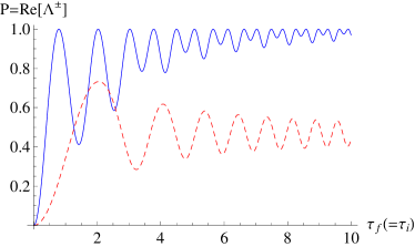
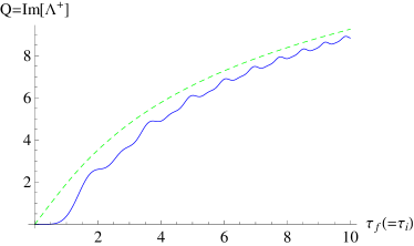
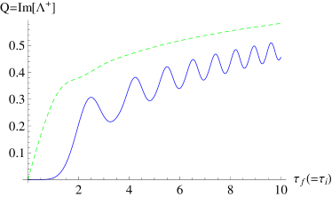
Figure 2: (a) Transition probability $P=\text{Re}\{\Lambda^{\pm}(\tau_{f})\}$ for a linear sweep starting in the $S$ state at the initial time $-\tau_{i}$ and ending at the final time $\tau_{f}=\tau_{i}$ plotted as a function of the half-sweep time $\tau_{f}$ for two values of the Landau-Zener parameter $\gamma$. Full (blue) line $\gamma=1$, dashed (red) line $\gamma=0.1$. The anticrossing point is passed in the middle of the sweep at time $\tau=0$. The full (blue) lines in (b) and (c) are $Q=\text{Im}\{\Lambda^{+}(\tau_{f})\}$ for $\gamma=1$ and $\gamma=0.1$, respectively. In (b) and (c), the dashed (green) lines are the adiabatic solutions of Eq. (54).

In agreement with the asymptotics found in Sec. V.2, the imaginary parts of $\Lambda^{\pm}$ displayed in Fig. 2(b,c) exhibit a behavior quite different from the behavior of their real parts $P$. They increase nearly logarithmically with $\tau_{f}$, with weak oscillations superimposed on this monotonic growth. Their magnitudes increase with $\gamma$, and for $\gamma\approx 1$ and $\tau_{f}\approx 10$ they are by one order of magnitude larger than $P$. Therefore, even with a moderate spin-orbit coupling, the imaginary parts of $\Lambda^{\pm}$ are expected to contribute essentially to the spin transfer $\Delta I^{z}$ of Eq. (26). This contribution should not only change the magnitude of $\Delta I^{z}$ but also smoothen its $\tau_{f}$-dependence.

In Fig. 2, we also plot $Q=\text{Im}\{\Lambda^{+}\}$ for $\gamma=1$ by using the approximate adiabatic expression of Eq. (54) to compare it to the exact numerical result. Apart from some details of the behavior for early and late times, which are expected, we see that the dominant contribution to $Q$ can be explained in terms of the adiabatic field of Eq. (54). Fig. 2 provides a similar comparison, but for a faster sweep with $\gamma=0.1$. Even in this situation, the adiabatic approximation is a reasonable starting point for describing the basic shape of $Q$ of Eq. 21.

The above analysis of linear sweeps, together with the arguments of Sec. V.4, allow to make some conclusions about the generic (non-linear) $S$-$T_{+}$ sweeps as well. Imagine the sweeps with the rate unchanged near the anticrossing but increasing away from it. As long as the speed-up happens at times $\tau>\tau_{tr}$ (this inequality should be fulfilled strong enough), the probability $P=\text{Re}\{\Lambda^{\pm}\}$ changes only modestly, while the long time tails of the products ${\tilde{c}}_{S}^{\ast}(\tau){\tilde{c}}_{T_{+}}(\tau)$ contributing to $Q=\text{Im}\{\Lambda^{+}\}$ are cut-off. Thus, increasing the sweep rate away from the anticrossing reduces $Q$ and might have a profound effect on $\Delta I^{z}$. However, its specific magnitude depends on the values of a number of parameters such as $v_{n}^{\pm},v_{so}^{\pm},\tau_{tr}$, and the speed-up time.

VI.2 Cyclic linear sweeps

Round sweeps are of the most practical interest for experiment, and their detailed shapes are nontrivial because of the oscillating tails of $\mathrm{Re}\{\Lambda^{\pm}\}$ of Fig. 2(a). Therefore, we provide below the data on $\Lambda^{\pm}$ for two different round sweeps starting in the singlet states $S$ at $\tau_{i}<0$.

Fig. 3 presents data for a round sweep of the total duration of $4\tau_{f}$ that includes the sweep of Fig. 2 from $\tau_{i}=-\tau_{f}$ to $\tau_{f}$ and the backward sweep that begins immediately after the end of the forward sweep. According to Eq. (20), $P=\mathrm{Re}\{\Lambda^{\pm}\}$ displays the probability of $S\rightarrow T_{+}$ transition. Remarkably, Fig. 3(a) shows that for $\gamma=1$ the decay of $P$ is rather long and includes deep and irregular oscillations. For $\gamma=0.1$, $P(\tau_{f})$ shows a wide maximum at $\tau_{f}\approx 2$, and the following oscillations without any visible decay up to $\tau_{f}=10$. In this case, a double dot in the linear sweep regime resembles a resonator of a length decreasing as $\tau_{f}^{-1}$. We expect that first peaks can be resolved experimentally, e.g., in beam splitter experimentsPetta2010 while higher peaks should merge into a background with $P\approx 0.5$. Using first sharp peaks for ultrafast spin operation is highly tempting.

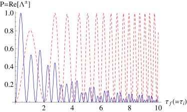
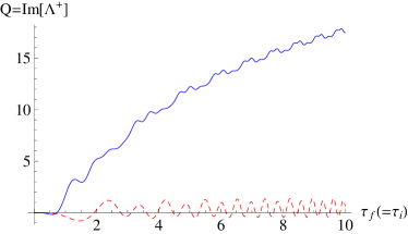
Figure 3: (a) Transition probability of a $S\rightarrow T_{+}$ transition $P=\text{Re}\{\Lambda^{\pm}\}$ and (b) the imaginary part $Q=\text{Im}\{\Lambda^{+}(\tau_{f})\}$ for a round sweep plotted versus $\tau_{f}$ (one fourth of the sweep time). The first part of the sweep is the same as the sweep of Fig. 2, and the second part sweeps in the opposite direction with the same speed immediately after reaching the turning point. Full (blue) lines $\gamma=1$, dashed (red) lines $\gamma=0.1$.

As distinct from $P=\mathrm{Re}\{\Lambda^{\pm}\}$, $Q=\mathrm{Im}\{\Lambda^{+}\}$ of Fig. 3(b) is a nearly monotonic function of $\tau_{f}$ for $\gamma=1$ (with irregular oscillations superimposed), and is about 10 for $\tau_{f}=10$. Therefore, it can heavily contribute to $\Delta I^{z}$. However, $\mathrm{Im}\{\Lambda^{\pm}\}$ is small and strongly oscillates at $\gamma=0.1$.

To demonstrate the effect of the tunneling process near the anticrossing point, in Fig. 4 are plotted the data for a cycle that begins in the $S$ state at $-\tau_{i}$, reaches the anticrossing at $\tau=0$, and then runs immediately back with the same speed until $\tau_{f}$ with $\tau_{i}=\tau_{f}$ . Comparison of Figs. 3(a) and 4(a) for $\gamma=1$ shows quite similar patterns of the oscillations of $P(\tau_{f})$ that are more regular in Fig. 4(a). However, the patterns for $\gamma=0.1$ are rather different demonstrating essential decrease in the spin transfer. The magnitudes of $Q=\mathrm{Im}\{\Lambda^{+}\}$ are small in both cases, but their $\tau_{f}$ dependences are rather different.

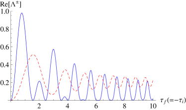
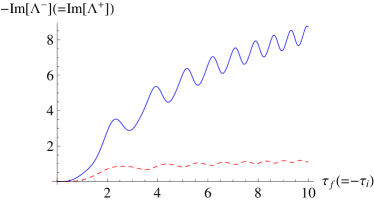
Figure 4: Real part $P$ (a) and imaginary part $Q$ (b) of the function $\Lambda^{+}(\tau_{f})$ for a round sweep plotted vs half-sweep time $\tau_{f}$. First part of the sweep, starting in the $S$ state at $\tau_{i}<\tau<0$, stops in the anticrossing point at $\tau=0$ and runs immediately in the opposite direction until $\tau_{f}=|\tau_{i}|$. Full (blue) lines $\gamma=1$, dashed (red) lines $\gamma=0.1$.

VI.3 Analytical theory of the probability oscillations

We can explain the oscillations in the transition probability as a function of the total duration of the cycle employing the analytical results in Sec. V. The forward sweep from $-\tau_{i}$ to the turning point $\tau_{m}$ gives rise to the singlet and triplet amplitudes of Eq. (44). Assuming $\tau_{m}\gg 1$ and $\tau_{i}\gg 1$, and employing (37a) and (37d), the singlet and triplet amplitudes at the turning point $\tau_{m}$ are

$$\tilde{c}_{S}^{(fS)} \approx e^{-\pi\gamma}e^{i\left(\tau_{i}^{2}-\tau_{m}^{2}\right)/4}\tau_{i}^{i\gamma}\tau_{m}^{-i\gamma},$$ (56)

$$\tilde{c}_{T_{+}}^{(fS)} \approx e^{-i3\pi/4}e^{-\pi\gamma/2}\frac{\sqrt{2\pi\gamma}}{\Gamma(1+i\gamma)}e^{i(\tau_{i}^{2}+\tau_{m}^{2})/4}\tau_{i}^{i\gamma}\tau_{m}^{i\gamma}.$$ (57)

Here the superscripts indicate that we started in the singlet $S$ state and carried out a forward linear sweep. The phase of the early time singlet state is arbitrary and is omitted because it only modifies the overall phase of the wave function and does not influence the final result for the probability. The amplitudes of Eqs. (56) and (57) are derived under the assumption that $\tilde{c}_{S}=1$ and $\tilde{c}_{T_{+}}=0$ at time $\tau=-\tau_{i}$.

Next, we consider the backward sweep and include the contributions from two channels passing through the $T_{+}$ and $S$ states at the turning point. As discussed in Sec. V.3, the dynamical equations for the amplitudes for the backward sweep $(\tilde{c}_{S}^{(b)},\tilde{c}_{T_{+}}^{(b)})$ differ from Eq. (16) by the interchange $\tilde{c}_{S}\longleftrightarrow\tilde{c}_{T_{+}}$. In order to make contact with our results in Sec. V, we change the time $\tau\rightarrow\tau-2\tau_{m}$ for the backward sweep. Using the interchange $\tilde{c}_{S}\longleftrightarrow\tilde{c}_{T_{+}}$, it follows from Eq. (44b) that for the triplet $T_{+}$ channel the ratio of the final and initial amplitudes along the backward sweep is $\tilde{c}_{S}^{(bT_{+})}/\tilde{c}_{T+}^{(fS)}=\sqrt{\gamma}e^{-i3\pi/8}D_{-1-i\gamma}\left(-e^{i\pi/4}\tau_{f}\right)/\left[e^{-i3\pi/8}D_{i\gamma}\left(-e^{i3\pi/4}\tau_{m}\right)\right]^{\ast}$, $T_{+}$ in the superscript of $\tilde{c}_{S}^{(bT_{+})}$ indicates the channel. In the limit $\tau_{f}\gg 1$, Eqs. (37d) and (37c) imply that this ratio equals

$$\tilde{c}_{S}^{(bT_{+})}/\tilde{c}_{T_{+}}^{(fS)}\approx e^{-i3\pi/4}e^{-\pi\gamma/2}\frac{\sqrt{2\pi\gamma}}{\Gamma(1+i\gamma)}e^{i(\tau_{f}^{2}+\tau_{m}^{2})/4}\tau_{f}^{i\gamma}\tau_{m}^{i\gamma}.$$ (58)

Similarly, by using the interchange $\tilde{c}_{S}\longleftrightarrow\tilde{c}_{T_{+}}$, it follows from Eq. (45b) that for the singlet $S$ channel the ratio of the final and initial amplitudes along the backward sweep $\tilde{c}_{S}^{(bS)}/\tilde{c}_{S}^{(fS)}=D_{i\gamma}\left(e^{3i\pi/4}\tau_{f}\right)/D_{i\gamma}\left(-e^{3i\pi/4}\tau_{m}\right)$. In the limit $\tau_{f}\gg 1,$ Eqs. (37d) and (37c) imply that the ratio of the singlet amplitudes after the backward sweep equals

$$\tilde{c}_{S}^{(bS)}/\tilde{c}_{S}^{(fS)}\approx e^{-\pi\gamma}e^{i(\tau_{f}^{2}-\tau_{m}^{2})/4}\tau_{f}^{i\gamma}\tau_{m}^{-i\gamma}\,.$$ (59)

The singlet amplitude at the final time $\tau_{f}$ after the cycle of duration $\left(\tau_{i}+\tau_{m}\right)+\left(\tau_{m}+\tau_{f}\right)$ is a sum of the contributions coming from both channels, $\tilde{c}_{S}^{(tot)}=\tilde{c}_{S}^{(bT_{+})}+\tilde{c}_{S}^{(bS)}$. Finally,

$$\tilde{c}_{S}^{(tot)} \approx e^{i\left(\tau_{f}^{2}+\tau_{i}^{2}-2\tau_{m}^{2}\right)/4}\left(\frac{\tau_{f}\tau_{i}}{\tau_{m}^{2}}\right)^{i\gamma}$$ (60)

$$\times\left[\left(1-P_{LZ}\right)+P_{LZ}e^{i\vartheta(\tau_{m})}\right],$$

where the Landau-Zener transition probability$P_{LZ}$ for a single-passage is defined by Eq. (46) and the phase $\vartheta(\tau_{m})$ at the turning point $\tau_{m}$ is defined as

$$e^{i\vartheta(\tau_{m})}=e^{i\tau_{m}^{2}}\tau_{m}^{4i\gamma}e^{-i\pi/2}\Gamma(-i\gamma)/\Gamma(i\gamma).$$ (61)

The dependence of the transition probability $P=1-\left|\tilde{c}_{S}(\tau_{f})\right|^{2}$ on the position $\tau_{m}$ of the turning point is

$$P(\tau_{m})=4P_{LZ}(1-P_{LZ})\sin^{2}\vartheta(\tau_{m})/2,$$ (62)

where $\vartheta(\tau_{m})$ is the Stückelberg phase.Stueckelberg ; ShimshoniGefen ; Shevchenko It is acquired between the two passages and includes both the adiabatic and non-adiabatic ($\gamma$-dependent) parts. From Eq. (62) we can make several observations that are consistent with the numerical data of Fig. 3. First, when $\tau_{f}\gg 1$ and $\tau_{i}\gg 1$, $P$ does not depend on the initial and final times. The transition probability only depends on the Landau-Zener probability $P_{LZ}$ of Eq. (46) and the turning point $\tau_{m}$. This means that the oscillations of $P(\tau_{m})$ are a robust feature of a coherent double passage across a Landau-Zener anticrossing. The transition probability oscillates around the average value

$$P_{av}=2P_{LZ}(1-P_{LZ}).$$ (63)

For fast sweeps $P_{LZ}\ll 1$ so that $P$ oscillates between $0$ and $4P_{LZ}$. For slow sweeps $P_{LZ}$ is close to $1$ and the probability oscillates between $0$ and $4(1-P_{LZ})$. The maximum in the oscillation amplitudes is achieved at $P_{LZ}=1/2$. When $P_{LZ}=1-e^{-2\pi\gamma}=1/2$ ($\gamma\approx 0.11$), the transition probability $P$ oscillates between $0$ and $1$. The amplitudes of the oscillations are smaller for all other values of $\gamma$. This is exacly the behavoir we see in the numerical plots. One more remarkable feature of Fig 3(a), that all oscillations pass through $P=0$, is also reflected by Eq. (62).

Oscillatory patterns of $\gamma=0.1$ curves in Figs. 2(a) and 3(a) show strikingly different behavior. In Fig. 2(a), the amplitude of oscillations decreases with $\tau_{f}$, and $P$ gradually approaches its Landau-Zener limit $P_{LZ}$. On the contrary, in Fig. 3(a) the oscillations, after some transitional period, acquire a stationary amplitude. Eqs. (62) and (63) clarify the origin of this behavior typical of double passages across the anticrossing.Stueckelberg ; ShimshoniGefen ; Shevchenko Indeed, $P_{av}$ of Eq. (63) is a Landau-Zener probability $P_{LZ}^{(2)}$ for a double passage across the anticrossing that can be derived directly by the above two-channel procedure with quantum amplitudes substituted by probabilities, see Ref. LL:book65, . Therefore, suppression of these long-time scale oscillations and approaching the double-passage Landau-Zener limit $P_{LZ}^{(2)}$ are only achieved when the decoherence is taken into account, and can allow measuring decoherence times.

In conclusion, prolonged oscillations of the electronic amplitudes $({\tilde{c}}_{S},{\tilde{c}}_{T_{+}})$ are a generic property of the coherent electron dynamics during the single- and double-passages across the $S$-$T_{+}$ anticrossing. Their amplitudes and durations are controlled by the Landau-Zener parameter $\gamma$ and by dephasing on longer time scales, and the patterns are rather different for the single- and double-passages.

VII Back action of nuclear spin dynamics on Overhauser fields

The Hamiltonian $\hat{H}$ of Eq. (3) describing the electron states depends on the Overhauser fields created by the spatially dependent nuclear spin configuration. The electrons experience the nuclear fields $v_{n}^{\alpha}$ and $\bm{\eta}_{n}$ of Eqs. (4) and (6), where the first represents the components of the effective difference magnetic field in the dots, and the second represents the induced average magnetic field. When going through the $S$-$T_{+}$ transition, the electrons will experience a change of these nuclear Overhauser fields. It is a unique property of Eq. (26) for the change in the total longitudinal nuclear spin $\Delta I^{z}$ that it expresses a global property of a double dot in terms of the parameters of the electronic Hamiltonian and does not depend of a specific configuration of nuclear spins. For different elements in the Hamiltonian $\hat{H}$, we calculate their mean-square values as well as their variances.

The expression for the change of the total $z$ component of the nuclear spin of  Eq. (27) makes the role of $Q$ explicit due to the mediation of spin-orbit coupling. With $v_{so}^{\pm}=0$, the total spin transfer is protected by the momentum conservation law and $Q$ manifests itself through shake-up processes in the nuclear spin reservoir respecting the conservation of the total angular momentum. The electron dynamics induces changes in the nuclear spin configuration that in turn induce changes in the in the diagonal and off-diagonal elements of the electron Hamiltonian (3). In what follows, we compute these changes.

VII.1 Changes in Overhauser fields

Electrons experience an effective Zeeman splitting in the Overhauser field of $\hat{\bm{\eta}}_{j}$ of Eq. (6). The associated change in the $z$-component of $\hat{\bm{\eta}}_{j}$, $\Delta{\hat{\eta}}_{n}^{z}=-A\sum_{j}\zeta_{j}\Delta{\hat{I}}_{j}^{z}$, is

$$\Delta{\hat{\eta}}_{n}^{z}=\frac{A^{2}}{2v_{\perp}^{2}}\sum_{j}\rho_{j}\zeta_{j}(\Lambda^{-}v^{-}{\hat{I}}_{j}^{+}+\Lambda^{+}v^{+}{\hat{I}}_{j}^{-}),$$ (64)

In the multicycle regime, the field of Eq. (64) has been measured by Petta et al.Petta2008 and by Foletti et al.Foletti:nphys09 by the shift in the position of the $ST_{+}$ anticrossing. In contrast to $\Delta I^{z}$, the change $\Delta{\hat{\eta}}_{n}^{z}$ in the longitudinal field depends on the detailed nuclear spin configuration and on the spatially dependent electron-nuclear couplings $\rho_{j}$ of Eq. (5) and $\zeta_{j}$ of Eq. (7).

The singlet-triplet terms ${\hat{v}}_{n}^{\pm}$ and ${\hat{v}}_{n}^{z}$ in the Hamiltonian $\hat{H}$ of Eq. (3) are sums over all nuclear spins. $ST_{0}$ level splittings characterized by ${\hat{v}}_{n}^{z}$ were measured in Ref. Petta2005, and a number of follow-up papers, and $ST_{+}$ splittings described by ${\hat{v}}_{n}^{\pm}$ in Ref. Petta2010, . The changes in these terms during a cycle are $\Delta{\hat{v}}^{\alpha}_{n}=A\sum_{j}\rho_{j}{\hat{I}}_{j}^{\alpha}$. By using Eq. (24), we find changes in the components $\alpha=\pm$ that couple $S$ to $T_{\pm}$

$$\Delta\hat{v}_{n}^{\pm} = \frac{A^{2}}{2v_{\bot}}\left[\frac{v^{\pm}}{v_{\bot}}\Lambda^{\pm}\sum_{j}\rho^{2}_{j}\hat{I}_{j}^{z}\pm i\Lambda^{z}\sum_{j}\rho_{j}\zeta_{j}\hat{I}_{j}^{\pm}\right]$$ (65)

$$\mp iA\sum_{j}\rho_{j}\frac{\eta_{j(nZ)}}{\hbar}(T_{f}-T_{i})\hat{I}_{j}^{\pm},$$

and, by using Eq. (25), in the component $\alpha=z$ coupling $S$ to $T_{0}$

$$\Delta\hat{v}_{n}^{z}=-\frac{A^{2}}{2v_{\bot}^{2}}\left[\Lambda^{-}v^{-}\sum_{j}\rho_{j}^{2}\hat{I}_{j}^{+}+\Lambda^{+}v^{+}\sum_{j}\rho^{2}_{j}\hat{I}_{j}^{-}\right].$$ (66)

We note that while ${\hat{v}}^{z}_{n}$ only produces a longitudinal Overhauser field mixing $S$ and $T_{0}$, $\Delta{\hat{v}}_{n}^{z}$ includes operators ${\hat{I}}^{\pm}_{j}$ and therefore mixes $S$ and $T_{+}$ belonging to our $2\times 2$ subspace.

In the next sub sections, mean values and variances of these operatores are computed.

VII.2 Constraints and mean values

While nuclear spins are distributed in the bath randomly, the magnetization fluctuations $v_{n}^{\pm}$ controlling electron dynamics during the cycle impose on their values the constraints

$$A\sum_{j}\rho_{j}I_{j}^{\alpha}=v_{n}^{\alpha},$$ (67)

adding also a constraint related to $v_{n}^{z}$. To simplify calculations, we consider below the nuclear spins $\mathbf{I}_{j}$ as random Gaussian variables that are normalized, in the absent of constraints, as $\langle I_{j}^{\lambda}I_{j^{\prime}}^{\lambda^{\prime}}\rangle=\frac{1}{3}I_{j}(I_{j}+1)\delta_{jj^{\prime}}\delta_{\lambda\lambda^{\prime}}$, with $\lambda=(x,y,z)$. Then the mean values of $I_{j}^{\lambda}$ are

$$\langle I_{j}^{\lambda}\rangle=\frac{\int dI_{j}^{\lambda}I_{j}^{\lambda}\mathcal{P}(I_{j}^{\lambda})\prod_{j^{\prime}\neq j}\int dI_{j^{\prime}}^{\lambda}\mathcal{P}(I_{j^{\prime}}^{\lambda})\delta(v_{n}^{\lambda}-A\sum_{j^{\prime}}\rho_{j^{\prime}}I_{j^{\prime}})}{\prod_{j^{\prime}}\int dI_{j^{\prime}}^{\lambda}\mathcal{P}(I_{j^{\prime}}^{\lambda})\delta(v_{n}^{\lambda}-A\sum_{j^{\prime}}\rho_{j^{\prime}}I_{j^{\prime}}^{\lambda})},$$ (68)

where $\mathcal{P}(I_{j}^{\lambda})$ are Gaussian probabilities, $(v_{n}^{x},v_{n}^{y})$ are defined as $v_{n}^{\pm}=(v_{n}^{x}\pm v_{n}^{y})/\sqrt{2}$, and the denominator secures the normalization of the probabilities under the constraints of Eq. (67).

Using the integral representation for $\delta$-functions

$$\delta(x)=\frac{1}{2\pi}\int_{-\infty}^{\infty}e^{i\omega x}d\omega,$$ (69)

multiple Gaussian integrations of Eq. (68) result in

$$\langle I^{\pm}_{j}\rangle=\rho_{j}v_{n}^{\pm}/(AR_{2}),\,\,\langle I^{z}_{j}\rangle=\rho_{j}v_{n}^{z}/(AR_{2}),$$ (70)

where $R_{n}=\sum_{j}\rho_{j}^{n}$ are determined by the spatial dependence of the electron-nuclear coupling constants. Substituting these expressions into Eqs. (64) and (65), we arrive at the corrections to the nuclear field experienced by the electron spin during the sweep.

$$\langle\Delta\eta^{z}_{n}\rangle=-\Delta I^{z}AR_{3}^{\prime}/R_{2},$$ (71)

where $R_{3}^{\prime}=\sum_{j}\rho^{2}_{j}\zeta_{j}$, and the Overhauser field mixing its $S$ and $T_{+}$ components

$$\langle\Delta v^{z}_{n}\rangle=-\Delta I^{z}AR_{3}/R_{2},$$ (72)

with $\Delta I^{z}$ of Eq. (26).

We see that both the changes in the longitudinal difference field $\Delta v_{n}^{z}$ and the longitudinal average field $\Delta\eta_{z}$ are proportional to the change in the total nuclear spin $\Delta I^{z}$. It follows from Eqs. (5) and (7) that $\rho_{j}$ typically have opposite signs in both dots while $\zeta_{j}>0$ everywhere, hence, $R_{3}^{\prime}>0$. Therefore, with $A>0$, the sign of $\langle\Delta\eta_{n}^{z}\rangle$ (the change in the mean Overhauser field building in the double dot) is opposite to the sign of $\Delta I^{z}$, in agreement with Eq. (6). The sign of $\langle\Delta v^{z}_{n}\rangle$ is defined by the sign $R_{3}$ that depends on the choice of electronic basis functions (see Appendix B), therefore, it is not uniquely defined with respect to $\Delta I^{z}$.

The magnitudes of $\Delta\eta_{z}$ and $\Delta v_{n}^{z}$ are of the order of $\Delta I^{z}An_{0}/N$ per cycle, i.e., about $\Delta I^{z}/\sqrt{N}$ of the mean values of $\eta_{z}$ and $v_{n}^{z}$. For $v_{so}^{\pm}=0$, $\Delta I^{z}=-P$, hence, $\mid\Delta I^{z}\mid\leq 1$. However, it is seen from Figs. 2(b) and 3(b) that $Q$ is an order of magnitude larger than $P$ when $\gamma\gtrsim 1$. Therefore, when $v_{so}\neq 0$, the conditional expectation values $\langle\Delta\eta_{n}^{z}\rangle$ and $\langle\Delta v_{n}^{z}\rangle$ should experience $Q$-enhancement through the $Q$-enhancement of $\Delta I^{z}$, and $\eta_{z}$ and $v_{n}^{z}$ can change by about 1% per cycle.

The mean values of the transverse components of $\mathbf{v}_{n}$, calculated in a similar way from Eq. (65), are

$$\langle\Delta v_{n}^{\pm}\rangle = A\frac{v^{\pm}v_{n}^{z}}{2v_{\perp}^{2}}\frac{R_{3}}{R_{2}}\Lambda^{\pm}\pm iA\frac{v_{n}^{\pm}}{2v_{\perp}}\frac{R_{3}^{\prime}}{R_{2}}\Lambda^{z}$$ (73)

$$\mp iv_{n}^{z}{\bar{\eta}}_{(nZ)}(T_{f}-T_{i})/\hbar$$

where ${\bar{\eta}}_{(nZ)}$ is a mean value of $\eta_{j(nZ)}$ over all nuclear species. Because different species are distributed randomly at the scale of atomic spacings, they self-average in the linear approximation over $T_{f}-T_{i}$, and we accept that all of them have the same absolute values of the angular momenta, $I_{j}=I$. While the first term is comparable in the magnitude to Eq. (72), the two last term might be much larger because they increase with the sweep duration. However, Eq. (73) includes changes both in the amplitude and the phase of $\Delta v_{n}^{\pm}$, and the latter might not be essential when solving Eq. (16) that only depends on $v_{\perp}$. We come back to this term in Sec.  VII.4.

VII.3 $ST_{+}$-pulses induced interdot shake-ups

Let us explain the importance of the variance in the spin production by considering the total nuclear spins in the left and right dots. Average values of different operators calculated in Sec. VII.2 were based on the conditional mean values $\langle I^{\alpha}_{j}\rangle$ of nuclear spins $I_{j}^{\alpha}$ of the order of $N^{-1/2}$ that are small compared with their root mean-square values. Therefore, calculating the mean-square values of all operators and their variances is important for estimating the widths of statistical distributions.

We begin with the differences in the spin polarizations of the left and right dots, $L$ and $R$, that are critical for spin manipulation. While division of a double dot into its left and right parts holds only when the overlap integral is small enough, cf. Appendix B, the results are instructive. Splitting Eq. (4) into sums over $L$ and $R$, we define partial sums

$$v^{\alpha}_{nL(R)}=A\sum_{j\in L(R)}\rho_{j}I^{\alpha}_{j}.$$ (74)

Their sums are $v^{\alpha}_{n}$ and are a subject to constrains of Eq. (67). However, their differences

$$u^{\alpha}_{n}=v^{\alpha}_{nL}-v^{\alpha}_{nR}$$ (75)

are free of any constraints. Using Eq. (25), the change in the left-right polarization difference is

$$\Delta I^{z}_{LR}=-\frac{1}{2v^{2}_{\perp}}(\Lambda^{-}v^{-}u^{+}_{n}+\Lambda^{+}v^{+}u^{-}_{n}).$$ (76)

When averaged over an unpolarized spin reservoir, its mean value vanishes, $\langle\Delta I^{z}_{LR}\rangle=0$, and the mean-square value equals

$$\langle(\Delta I^{z}_{LR})^{2}\rangle=\frac{A^{2}n_{0}}{6v_{\perp}^{2}}I(I+1)\mid\Lambda\mid^{2}\int\rho^{2}(\mathbf{R})d^{3}\mathbf{R},$$ (77)

with $\rho(\mathbf{R})$ of Eq. (5) and

$$\mid\Lambda\mid^{2}=P^{2}+Q^{2}.$$ (78)

A simple estimate of the right hand side of Eq. (77) results in $\mid\Lambda\mid^{2}$. Therefore, the asymmetry of spin pumping of the left and right dots is $Q$-enhanced whenever $Q\gg P$, in particular, when $v_{so}=0$ and $P\leq 1$. We attribute this enhancement to shake-up processes resulting in multiple spin flips per each “pure” injected nuclear spin. These processes are random, and it is not clear for now how they influence inhomogeneous spin distributions.Ramon:prb07 ; Gullans:prl10

The detailed spatial patterns of spin generation at long time scales are a subtle subject and are related to the spatial variation of the electron-nuclear couplings $\rho(\mathbf{R}_{j})$ and $\zeta(\mathbf{R}_{j})$ calculated in Appendix B. With mean values of $I_{j}^{\pm}$ of Eq. (70), spatial distribution of $\Delta I_{j}^{z}$ is related to $\Delta I^{z}$ as $\Delta I_{j}^{\pm}=(\rho_{j}^{2}/R^{2})\Delta I^{z}$. The left-right asymmetry in $\rho_{j}^{2}$ originates either from the geometric asymmetry of the double dotGullans:prl10 or from the $L$-$R$-overlap of the electron density, cf. Appendix B, and produces a regular difference in the $I^{z}$ generation rate. While the results depend on the specific distribution of nuclear spins and the $S$-$T_{0}$ mixing,Stopa:prb10 the mechanism of $Q$-enhancement is quite general whenever $\gamma\gtrsim 1$.

VII.4 Mean-square values and variances

Mean values of Sec. VII.2 were evaluated over an unpolarized nuclear spin bath and estimate the mean rates of the change of the different parameters. However, the estimate of the shake-up rate of Sec. VII.3 demonstrates that calculating variances of these random variables can provide additional, and sometimes even more valuable, information about the magnitudes of the expected changes during a cycle. The conditional probability distributions are so wide that the mean value is not very representative. In this section, we evaluate variances of the basic nuclear fields.

We begin with calculating the mean-square values. Because all nuclear fields of Eqs. (64) - (66) are linear in the momenta $I^{\alpha}_{j}$, mean values of the quadratic forms in them include integrals that differ from Eq. (68) by substituting $I^{\lambda}_{j}$ either by $(I^{\lambda}_{j})^{2}$ or by $I^{\lambda}_{j}I^{\lambda}_{j^{\prime}}$ with $j\neq j^{\prime}$. While the latter terms are smaller in the parameter $1/N\ll 1$, they have a higher statistical weight. Summing all terms, one arrives at length expressions for $\langle(\Delta\eta_{n}^{z})^{2}\rangle$ and $\langle(\Delta v_{n}^{z})^{2}\rangle$ that we do not present here. Instead, using the mean values of Eqs. (71) and (72), we present the variances defined as $\mathrm{Var}\{\mathrm{\xi}\}=\langle\xi^{2}\rangle-\langle\xi\rangle^{2}$

$$\mathrm{Var}\left\{\Delta{\eta}^{z}_{n}\right\}=\mid\Lambda\mid^{2}\frac{A^{4}}{6v_{\perp}^{2}}I(I+1)[R_{4}^{\prime}-(R_{3}^{\prime})^{2}/R_{2}],$$ (79)

where $R_{4}^{\prime}=\sum_{j}(\rho_{j}\zeta_{j})^{2}$, and

$$\mathrm{Var}\left\{\Delta{v}_{n}^{z}\right\}=\mid\Lambda\mid^{2}\frac{A^{4}}{6v_{\perp}^{2}}I(I+1)[R_{4}-(R_{3})^{2}/R_{2}].$$ (80)

Comparison with Eqs. (71) and (72) shows $Q$-enhancement even when $v_{so}=0$ (hence, when $\Delta I=-P)$, the effect that manifested itself already in Eq. (77). This means that the nuclear spins with $I_{j}^{z}$ away from the mean conditional expectation values $\langle I_{j}^{z}\rangle$ respond to the sweeps stronger than the spins with $I_{j}^{z}=\langle I_{j}^{z}\rangle$. Also, this enhanced sensitivity is due to the spatial distribution of $\rho_{j}$ and $\zeta_{j}$ because with $\rho_{j}$=const and $\zeta_{j}$=const the brackets in Eqs. (79) and (80) vanish. By the order of magnitude, both quantities experience changes of about $\Lambda An_{0}/N$ per cycle; with $\Lambda\approx 10$ and $N\approx 10^{6}$, this suggests changes about 1% per cycle. In other words, around 10 spins interchange their directions during one passage.

Calculating $\langle\Delta(v_{n}^{+}v_{n}^{-})\rangle$ results in a simple equation

$$\langle\Delta(v_{n}^{+}v_{n}^{-})\rangle=-I^{z}Av_{n}^{z}R_{3}/R_{2}$$ (81)

because the contributions of the two last terms of Eq. (65) cancel. In absence of spin-orbit coupling, this immediately suggests $\langle\Delta(v_{\perp}^{2})\rangle=PAv_{n}^{z}R_{3}/R_{2}$. Under these conditions, large terms in Eq. (65) reflect only the change in the phase of $v_{n}^{\pm}$ that does not influence dynamical equations (16), and the relative change in $(v_{n}^{\perp})^{2}=v_{n}^{+}v_{n}^{-}$ is only about $N^{-1/2}$.

However, in presence of spin-orbit coupling the dynamics of spin amplitudes $({\tilde{c}}_{S},{\tilde{c}}_{T})$ is controlled by $v^{\pm}$ rather then $v_{n}^{\pm}$. Mean value of $\Delta(v_{\perp}^{2})$, calculated by using Eqs. (65) and (70), is

$$\langle\Delta(v^{+}v^{-})\rangle=\langle\Delta(v_{n}^{+}v_{n}^{-})\rangle$$

$$+ \frac{Av_{n}^{z}}{2v_{\perp}^{2}}\frac{R_{3}}{R_{2}}[\Lambda^{-}v_{n}^{-}v_{so}^{+}+\Lambda^{+}v_{n}^{+}v_{so}^{-}]$$

$$+ i(v_{n}^{-}v_{so}^{+}-v_{n}^{+}v_{so}^{-})\left[\frac{{\bar{\eta}}_{nB}}{\hbar}(T_{f}-T_{i})-\frac{A}{2v_{\perp}}\frac{R_{3}^{\prime}}{R_{2}}\Lambda^{z}\right],$$

where first term is defined by Eq. (81). Physically, second and third terms in Eq. (VII.4) take into account the angle between $v_{n}^{+}$ and $v_{so}^{+}$ in the complex plane, and are proportional to the product $v_{\perp}v_{n}^{\perp}$. With $v_{\perp}\sim v_{n}^{\perp}$, relative corrections coming from the second term are of the order $\Lambda/\sqrt{N}$ per cycle. The third term is usually much larger because it increases linearly with the pulse duration $\Delta T=T_{f}-T_{i}$. It includes two contributions of which first is due to the Zeeman precession of nuclei and second due to the Knight field and is proportional to the integral of $\mid{\tilde{c}}_{T+}\mid^{2}$. While the magnitude of the second contribution depends on the shape of the pulse, the ratio of these terms is roughly ${\bar{\eta}}_{(nB)}/(An_{0}/N)$ and they become comparable at $B\sim 1$ mT. This indicates that first contribution to the third term usually dominates. With $v_{\perp}\sim v_{so}^{\perp}$ and ${\bar{\eta}}_{(nB)}\approx 10$ mT, the Zeeman term results in $\langle\Delta(v^{+}v^{-})\rangle\sim 0.1\langle v^{+}v^{-}\rangle$ for a 0.1$\mu$s linear sweep. This is much larger than the correction to the same quantity estimated in Eq. (81) and to $\langle(\Delta v_{n}^{z})^{2}\rangle$ having the same scale. The effect in InAs should be much larger than in GaAs because of the stronger spin-orbit coupling.

The above estimates indicate that, because of the terms in Eq. (65) linear in the pulse duration, spin-orbit corrections to transverse matrix elements are essentially larger than the corrections to the longitudinal ones.

In Eq. (VII.4), Zeeman precession of nuclei manifests itself in $\langle(v^{+}v^{-})\rangle$ only through spin-orbit coupling. The effect is much stronger when estimated through the variance of $v^{+}v^{-}$, and we estimate it for $v_{so}=0$ when $v^{\pm}=v_{n}^{\pm}$. Disregarding two first terms in Eq. (65), the calculations similar to those performed above when deriving Eqs. (79) and (80) result in

$$\mathrm{Var}\{\Delta(v_{n}^{+}v_{n}^{-})\} \approx \frac{I(I+1)}{6}(\overline{\eta^{2}_{(nB)}}-{\bar{\eta}_{(nB)}}^{2})$$ (83)

$$\times (v_{n}^{+}v_{n}^{-})A^{2}R_{2}[(T_{f}-T_{i})/\hbar]^{2},$$

where $\overline{\eta^{2}_{(nB)}}$ is the mean-square value of $\eta_{j(nB)}$. It follows from Eq. (83), the dominating mechanism of changing $v_{n}^{\perp}$ is the nuclear spin precession with a characteristic time of about a microsecond at $B\sim 10$ mT. It is about two to three orders of magnitude shorter than the corresponding time for $v_{n}^{z}$ estimated above.

It is also instructive to compare this estimate with a much longer time for $v_{n}^{\perp}$ following from Eq. (81). The latter estimate was found with the nuclear configuration of Eq. (70) that reflects the mean-values of nuclear spins under the constraints of Eq. (67). In a narrow region of the phase space around these mean values dynamics of $v_{n}^{\perp}$ is strongly suppressed. The estimate of Eq. (83) is much more representative because it represents the entire phase space compatible with the constraints of Eq. (67). A similar type of the behaviour of $v_{n}^{z}$ was discussed above as applied to Eq. (80).

VIII Conclusions

We have studied the dynamics of the electron and nuclear spins near $ST_{+}$ avoided crossings in double quantum dots. While adopting the traditional approach based on the hierarchy of time scales, with a slow nuclear and fast electron dynamics, we employed a quantum description of the electron spin and coherent dynamics of nuclear spins, and investigated the time-resolved patterns of single and double Landau-Zener passages through the anticrossing point. They are described by two complex conjugate functions $\Lambda^{\pm}$ depending on the initial and finite times $(T_{i},T_{f})$ and the trajectory of the sweep, with $\Lambda^{-}$ proportional to the integral of the product ${\tilde{c}}_{S}^{\ast}(t){\tilde{c}}_{T}(t)$ of the complex amplitudes of the $S$ and $T_{+}$ states. Their real parts $P=\mathrm{Re}\{\Lambda^{\pm}\}$ are proportional to the $S$-$T_{+}$-transition probability and for one-side sweeps oscillate at small time scales when the system is close to the anticrossing and saturate at long time scales. For linear sweeps, we find the singlet and triplet amplitudes in terms of Weber $D$-functions (parabolic cylinder functions); the long-time asymptotic limit of $P$ equals the Landau-Zener probability $P_{LZ}=1-e^{-2\pi\gamma}$. For round trips, the system also experiences long-term Stückelberg oscillations. The first sharp oscillations might be utilized for ultrafast electron spin operation, while the decay of the oscillations can provide information about dephasing rates. It is important that the imaginary part $Q=\mathrm{Im}\{\Lambda^{+}\}$ that acquires contributions from the electronic states at a wide time scale and accumulates with time (it diverges logarithmically for linear sweeps) has a profound effect on the dynamics of the nuclear spins. When the Landau-Zener parameter $\gamma\gtrsim 1$, $Q$ is typically one order of magnitude larger than $P$. Therefore, in presence of the spin-orbit coupling violating the angular momentum conservation, $Q$ may become the major factor controlling the angular momentum transfer to nuclei. In particular, this mechanism is efficient for excursions including a stay near the anticrossing point. Generically, $\Lambda=(P^{2}+Q^{2})^{1/2}$ controls the shake-up processes that exchange angular momentum between the left and right dots. With $Q\gg P$, it is $Q$ that plays a dominating role in these angular-momentum exchange processes. Because the mechanism that plagues many experimental efforts of building considerable polarization gradients remains unknown, it is a challenging question whether and how the shake-up processes contribute to it; unfortunately, only a theory including multiple passages can resolve it. We also estimated changes in the Overhauser fields during a single cycle and concluded that the transverse components are more volatile than the longitudinal ones.

We are grateful to B. I. Halperin, C. M. Marcus, I. Neder, and M. Rudner for stimulating discussions and comments on the manuscript. E. I. R. was funded by IARPA through the Army Research Office, by NSF under Grant No. DMR-0908070, and in part by Rutherford Professorship (Loughborough, UK).

Appendix A Spin Operator

We use the following convention for the spin-1 operator $\mathbf{S}$

$$S_{x} = \frac{1}{\sqrt{2}}\left(\begin{array}[]{ccc}0&1&0\\ 1&0&1\\ 0&1&0\end{array}\right),$$ (87)

$$S_{y} = \frac{1}{\sqrt{2}}\left(\begin{array}[]{ccc}0&-i&0\\ i&0&-i\\ 0&i&0\end{array}\right),$$ (91)

$$S_{z} = \left(\begin{array}[]{ccc}1&0&0\\ 0&0&0\\ 0&0&-1\end{array}\right).$$ (95)

These operators satisfy the commutation relations$\left[\hat{S}_{i},\hat{S}_{j}\right]=i\epsilon_{ijk}\hat{S}_{k}$, where $\ \epsilon_{ijk}$ is the Levi-Civita tensor, as well as$\ \hat{S}_{x}^{2}+\hat{S}_{y}^{2}+\hat{S}_{z}^{2}=2$.

Appendix B Simple Model

The singlet part of the spin wave function is

$$\chi_{S}(1,2)=\frac{1}{\sqrt{2}}\left(|\uparrow_{1}\rangle|\downarrow_{2}\rangle-|\downarrow_{1}\rangle|\uparrow_{2}\rangle\,\right)$$ (96)

and the three triplet components of the spin wave function are

$$\,\chi_{T_{+}}(1,2) =|\uparrow_{1}\rangle|\uparrow_{2}\rangle,$$ (97a)

$$\chi_{T_{0}}(1,2) =\frac{1}{\sqrt{2}}\left(|\uparrow_{1}\rangle|\downarrow_{2}\rangle+|\downarrow_{1}\rangle|\uparrow_{2}\rangle\right),$$ (97b)

$$\chi_{T_{-}}(1,2) =|\downarrow_{1}\rangle|\downarrow_{2}\rangle.$$ (97c)

We will in this section discuss the spatial dependence of the hyperfine coupling constants $\rho_{j}$ of Eq. (5) and $\zeta_{j}$ of Eq. (7). In a simple model, the electron wave functions near the $S$-$T_{+}$ anticrossing are

$$\psi_{S}(1,2) = \cos\nu~{}\psi_{R}(1)\psi_{R}(2)$$ (98)

$$+ \frac{\sin\nu}{\sqrt{2}}[\psi_{L}(1)\psi_{R}(2)+\psi_{L}(2)\psi_{R}(1)],$$

$$\psi_{T}(1,2)=\frac{1}{\sqrt{2}}[\psi_{L}(1)\psi_{R}(2)-\psi_{L}(2)\psi_{R}(1)],$$ (99)

where $L$ denotes the left and $R$ the right dot, and the angle $\nu$ depend on the Zeeman energy $\eta_{Z}$. The normalization coefficients in (98) and (99) are exact under the assumption that the functions $\psi_{L}$ and $\psi_{R}$ are orthonormalized.

Let us illustrate the spatial dependence of the electron-nuclear coupling constants $\rho$ of Eq. (5) and $\zeta$ of Eq. (7) for a simple model of a quantum dot. We assume the electrons are in the lowest orbital harmonic oscillator state. The Cartesian coordinates, the wave function is $\psi(x,y)=\exp\left[-(x^{2}+y^{2})/l^{2}\right]/(l\sqrt{2/\pi})$, where $l$ is the size of each quantum dot. We have two quantum dots that are separated at a distance $d$, one at $x=-d/2$ and $y=0$ and the other at $x=d/2$ and $y=0$. We form an orthonormal basis set based on the functions $\psi(x-d/2,y)$ and $\psi(x+d/2,y)$. In this basis, we compute $\rho(x,y)$ and $\zeta(x,y)$.

We plot in Fig.  5 the electron-nuclear couplings $\rho(x,y)$ and $\zeta(x,y)$ for $y=0$ as a function of $x$ when $\nu=0.1$ and $\nu=\pi/2-0.1$. The spatial distribution of the singlet-triplet coupling $\rho(x,y)$ depends on the angle $\nu$. When $\nu$ is close to $\pi/2$, there is a nearly equal probability for electrons to be located in the left and right dot for both the singlet and triplet states. Then the singlet-triplet coupling $\rho(x,y)$ is nearly antisymmetric around $x=0$, $\rho(x,y)\approx-\rho(-x,y)$ [the sign of $\rho(x,y)$ depends on the sign choice in Eq. (99)]. When $\nu$ is small, the electrons are in the singlet state $(0,2)$ in the right dot,   so that $\rho(x,y)$ passes through zero inside the right dot (for $x>0$). Therefore, even for two symmetrically shaped dots, the $S$-$T_{+}$ electron-nuclear coupling can become asymmetric because of the overlap of the left and the right dot wave functions. The asymmetry depends on $\nu$ controlled by the external magnetic field.

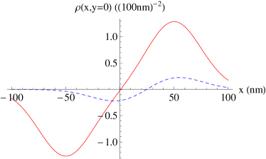
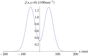
Figure 5: The spatial variation of the electron-nuclear couplings $\rho(x,y=0)$ (a) and $\zeta(x,y=0)$ (b). In (a), the red (full) curve is for $\nu=\pi/2-0.1$ and the blue (dashed) curve is for $\nu=0.1$. The size of the dots is $l=50$ nm and the separation between the dots is $d=100$ nm. The overlap integral between the left and the right oscillator wave function is $0.1$. It is the most striking feature that the overlap between the wave functions induces asymmetry of the $\rho(x,y)$ even in geometrically symmetric double dots. The asymmetry reaches its maximum when the system is close to the $(0,2)$ state.

The triplet-triplet electron-nuclear coupling $\zeta(x,y)$ does not depend on $\nu$ and is a symmetric function of $x$ for the two symmetric quantum dots.

Appendix C Two identities for the parabolic cylinder $D$-functions

Using the solution of Eq. (44) for ${\tilde{c}}_{T_{+}}(\tau)$ and ${\tilde{c}}_{S}(\tau)$ and the normalization condition $|{\tilde{c}}_{S}(\tau)|^{2}+|{\tilde{c}}_{T_{+}}(\tau)|^{2}=1$, we arrive at an identity

$$\gamma\mid D_{-1-i\gamma}(-e^{i\pi/4}\tau)\mid^{2}+\mid D_{i\gamma}(e^{i3\pi/3}\tau)\mid^{2}=e^{\pi\gamma/2}$$ (100)

relating absolute values of two $D$-functions at arbitrary real values of $\tau$ and $\gamma$.

Next, it follows from Eq. (29) that

$$\partial_{\tau}\left(\mid{\tilde{c}}_{S}\mid^{2}-\mid{\tilde{c}}_{T_{+}}\mid^{2}\right)=-2i\sqrt{\gamma}\left({\tilde{c}}_{S}^{*}{\tilde{c}}_{T_{+}}-{\tilde{c}}_{S}{\tilde{c}}_{T_{+}}^{*}\right).$$ (101)

Integrating it over $\tau$ and using Eqs. (44) and (46), we find

$$\int_{-\infty}^{\infty}d\tau~{}\mathrm{Im}\{e^{-i3\pi/4}D_{-1-i\gamma}(-e^{i\pi/4}\tau)D_{i\gamma}(e^{i3\pi/4}\tau)\}$$ (102)

$$= -\frac{\sinh\pi\gamma}{\gamma}e^{-\pi\gamma/2}.$$

The integral of the real part of the integrand diverges.

While we could not find these identities for $D_{n}(z)$ functions with complex (imaginary) indeces $n$ and the arguments directed along diagonals in the complex $z$ planes in any of mathematical sources, we checked them numerically.

References

- (1) R. Hanson, L. P. Kouwenhoven, J. R. Petta, S. Tarucha, and L. M. K. Vandersypen, Rev. Mod. Phys. 70, 1217 (2007).
- (2) D. Loss and D. P. DiVincenzo, Phys. Rev. A 57, 120 (1998).
- (3) J. Levy, Phys. Rev. Lett. 89, 147902 (2002).
- (4) I. A. Merkulov, Al. L. Efros, and M. Rosen, Phys. Rev. B 65, 205309 (2002).
- (5) A. Khaetskii, D. Loss, and L. Glazman, Phys. Rev. B 67, 195329 (2003).
- (6) S. I. Erlingsson and Yu. V. Nazarov, Phys. Rev. B 70, 205327 (2004).
- (7) W. Yao, R.-B. Liu, and L. J. Sham, Phys. Rev. B 74, 195301 (2006).
- (8) L. Cywiński, W. M. Witzel, and S. Das Sarma, Phys. Rev. Lett. 102, 057601 (2009).
- (9) S. Foletti, H. Bluhm, D. Mahalu, V. Umansky, and A. Yacoby, Nat. Phys. 5, 903 (2009).
- (10) H. Bluhm, S. Foletti, D. Mahalu, V. Umansky, and A. Yacoby, Phys. Rev. Lett. 105, 216803 (2010).
- (11) H. Bluhm, S. Foletti, I. Neder, M. Rudner, D. Mahalu, V. Umansky, and A. Yacoby, Nat. Phys. 7, 109 (2011).
- (12) C. Barthel, D. J. Reilly, C. M. Marcus, M. P. Hanson, and A. C. Gossard, Phys. Rev. Lett. 103, 160503 (2009).
- (13) G. Ramon and X. Hu, Phys. Rev. B 75, 161301 (R) (2007).
- (14) M. Stopa, J. J. Krich, and A. Yacoby, Phys. Rev. B 81, 041304(R) (2010).
- (15) M. Gullans, J. J. Krich, J. M. Taylor, H. Bluhm, B. I. Halperin, C. M. Marcus, M. Stopa, A. Yacoby, and M. D. Lukin, Phys. Rev. Lett. 104, 226807 (2010).
- (16) M. S. Rudner and L. S. Levitov, Phys. Rev. B 82, 155418 (2010).
- (17) M. S. Rudner, I. Neder, L. S. Levitov, and B. I. Halperin, Phys. Rev. B 82, 041311 (2010).
- (18) H. Ribeiro and G. Burkard, Phys. Rev. Lett. 102, 216802 (2009).
- (19) W. Lu et al., Nature (London) 423, 422 (2003; J. M. Elzerman et al., Nature (London) 430, 431 (2004); T. Meunier et al., Phys. Rev. B 74, 195303 (2006); S. Amasha et al., Phys. Rev. Lett. 100, 046803 (2008).
- (20) J. R. Petta, H. Lu, and A. C. Gossard, Science 327, 669 (2010).
- (21) C. Zener, Proc. Roy. Soc. (London), Series A, 137, 696 (1932).
- (22) J. M. Taylor, H. A. Engel, W. Dur, A. Yacoby, C. M. Marcus, P. Zoller, and M. D. Lukin, Nat. Phys. 1, 177 (2005).
- (23) J. M. Taylor, J. R. Petta, A. C. Johnson, A. Yacoby, C. M. Marcus, and M. D. Lukin, Phys. Rev. B 76, 035315 (2007).
- (24) J. R. Petta, A. C. Johnson, J. M. Taylor, E. A. Laird, A. Yacoby, M. D. Lukin, C. M. Marcus, M. P. Hanson, and A. C. Gossard, Science 309, 2180 (2005).
- (25) M.P. Nowak, B. Szafran, F.M. Peeters, B. Partoens, and W. Pasek, arXiv:1102.1002.
- (26) D. V. Bulaev and D. Loss, Phys. Rev. B 71, 205324 (2005)
- (27) A. V. Khaetskii and Y. V. Nazarov, Phys. Rev. B 61, 12639 (2000).
- (28) A. Pfund, I. Shorubalko, K. Ensslin, and R. Leturcq, Phys. Rev. B 76, 161308 (2007).
- (29) S. Takahashi, R. S. Deacon, K. Yoshida, A. Oiwa, K. Shibata, K. Hirakawa, Y. Tokura, and S. Tarucha, Phys. Rev. Lett. 104, 246801 (2010).
- (30) E. I. Rashba and V. I. Sheka, in Landau Level Spectroscopy 1991 (North-Holland, Amsterdam), p. 131.
- (31) V. N. Golovach, M. Borhani, and D. Loss, Phys. Rev. B 74, 165319 (2006).
- (32) K. C. Nowack, F. H. L. Koppens, Y. V. Nazarov, and L. M. K. Vandersypen, Science 318, 1430 (2007).
- (33) M. Pioro-Ladrière, T. Obata, Y. Tokura, Y.-S. Shin, T. Kubo, K. Yoshida, T. Taniyama, and S. Tarucha, Nature Physics 4, 776 (2008).
- (34) S. Nadj-Perge, S. M. Frolov, E. P. A. M. Bakkers, and L. P. Kouwenhoven, Nature, 468, 1084 (2010).
- (35) E. I. Rashba, J. Supercond. Novel Magnetism, 18, 137 (2005).
- (36) E. A. Laird, C. Barthel, E. I. Rashba, C. M. Marcus, M. P. Hanson, and A. C. Gossard, Phys. Rev. Lett. 99, 246601 (2007).
- (37) We are grateful to M. Rudner for his help in establishing this connection.
- (38) L. D. Landau and E. M. Lifshitz, Quantum Mechanics (Pergamom, London, 1965) §90.
- (39) E. T. Whittaker and G. N. Watson, A Course of Modern Analysis (New York, MacMilland, 1945).
- (40) Higher Transcendental Functions, ed. by Erdélyi (Mc. Graw-Hill, New York, 1953), Chapter 8.
- (41) In Zener’s paper Zener:prs32 , the aymptotics of Ref. WhittakerWatson:book45 have been used. Fortunately, this did not influence his final result for the Landau-Zener transition probability.
- (42) J. R. Petta, J. M. Taylor, A. C. Johnson, A. Yacoby, M. D. Lukin, C. M. Marcus, M. P. Hanson, and A. C. Gossard, Phys. Rev. Lett. 100, 067601 (2008).
- (43) S. Foletti, J. Martin, M. Dolev, D. Mahalu, V. Umansky, and A. Yacoby, arXiv:0801.3613.
- (44) E. C. G. Stückelberg, Helv. Phys. Acta 5, 369 (1932).
- (45) E. Shimshoni and Y. Gefen, Ann. Phys. (NY) 210, 16 (1991).
- (46) S. N. Shevchenko, S. Ashhab, F. Nori, Phys. Rep. 492, 1 (2010).