Some remarks on the inverse Smoluchowski problem for cluster-cluster aggregation

Abstract

It is proposed to revisit the inverse problem associated with Smoluchowski’s coagulation equation. The objective is to reconstruct the functional form of the collision kernel from observations of the time evolution of the cluster size distribution. A regularised least squares method originally proposed by Wright and Ramkrishna (1992) based on the assumption of self-similarity is implemented and tested on numerical data generated for a range of different collision kernels. This method expands the collision kernel as a sum of orthogonal polynomials and works best when the kernel can be expressed exactly in terms of these polynomials. It is shown that plotting an “L-curve” can provide an a-priori understanding of the optimal value of the regularisation parameter and the reliability of the inversion procedure. For kernels which are not exactly expressible in terms of the orthogonal polynomials it is found empirically that the performance of the method can be enhanced by choosing a more complex regularisation function.

I Introduction

The effects of clouds and precipitation is one of the largest sources of uncertainty in our current attempts to simulate the Earth’s climate STE2005 . The reason for this is that most phenomena associated with clouds happen on scales below those which are explicitly resolved by the current climate models. Their feedback on resolved scales must therefore be parameterised. Such parameterisations require a strong understanding of the underlying physical processes taking place. One such process which has attracted considerable attention in recent years is the time evolution of the droplet size distribution in clouds and its connection with precipitation. Water droplets in clouds are seeded by cloud condensation nucleii such as aerosol particles. They initially grow by condensation and subsequently by coagulation as droplets collide with each other in the cloud to produce larger droplets. The detailed micro-physics of the coagulation process is difficult to understand theoretically since turbulence within the cloud is believed to play a key role in determining the collision rate of droplets BMSS2010 . A complete theoretical description is hampered by the difficulty in describing the statistical interplay between particles and turbulence analytically. On the other hand the quality of the data available for the study of this problem is improving rapidly due to recent advances in observational techniques SLWF2006 and direct numerical simulation of droplets in turbulent flows RC2000 ; WARG2008 .

In the context of the droplet coagulation problem, much research has focused on using our improved observational understanding of the behavious of droplets in turbulent flows to calculate more accurately the functional form of the droplet coagulation rate, $K(m_{1},m_{2})$, as a function of droplet masses, or equivalently (if droplets are assumed spherical), droplet size. In this note, we argue that the improved availability of data suggests that we should also revisit the corresponding inverse problem which can be stated as follows: given observations or measurements of the time evolution of the droplet size distribution, how much information can be extracted about the functional form of the coagulation rate? This problem was studied in the past by Wright and Ramkrishna WR1992 in the context of chemical mixing and has been recently revisited in the context of droplets in turbulence by Onishi et al. OMTKK2011 . Although there are many difficulties associated with such inverse problems, as discussed below, there are potential rewards. The approach is data driven and could provide a guide to modeling in situations where the underlying microphysics remains incompletely understood. The inverse approach could also begin to quantify the extent to which available data and measurements can distinguish between different models.

First a word about the usual forward problem. If the collision kernel, $K(m_{1},m_{2})$, is known, the evolution of the cluster size distribution, $N_{m}(t)$ is described by the Smoluchowski coagulation equation SMO1917 :

$$\partial_{t}N_{m}(t) = \int_{0}^{m}dm_{1}\,K(m_{1},m-m_{1})\,N_{m_{1}}(t)\,N_{m-m_{1}}(t)$$ (1)

$$- 2N_{m}(t)\int_{0}^{\infty}dm_{1}\,K(m,m_{1})\,N_{m_{1}}(t).$$

It is applicable when spatial correlations between particles are sufficiently weak that collisions between particles can be considered statistically independent. A huge amount is known theoretically about the solutions of the Smoluchowski equation. See LEY2003 for a modern review.

II Homogeneous collision kernels and self-similarity

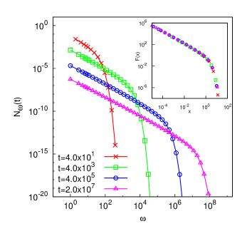
Figure 1: Snapshots of the self-similar evolution of the cluster size distribution, $N_{m}(t)$, obtained from a numerical simulation of Eq. (1) with the collision kernel $K(m_{1},m_{2})=(m_{1},m_{2})^{\frac{1}{4}}$. The inset shows the scaling function obtained when the data is collapsed according to Eq. (2) with the typical scale, $s(t)$, obtained as in Eq. (3) with $n=2$.

In some applications (see ERN1986 for some discussions), the collision kernel is a homogeneous function of its arguments whose degree we shall denote by $\gamma$:

$$K(am_{1},am_{2})=a^{\gamma}\,K(m_{1},m_{2}).$$

For such kernels, the evolution of the cluster size distribution is often self-similar. That is to say we can write:

$$N_{m}(t)\sim s(t)^{-2}\,f\left(z\right)\hskip 28.45274ptz=\frac{m}{s(t)}$$ (2)

where $s(t)$ is the typical cluster size. This can be defined intrinsically as a ratio of moments of the size distribution:

$$s(t)=\frac{M_{n+1}(t)}{M_{n}(t)}\hskip 28.45274ptM_{p}(t)=\int_{0}^{\infty}m^{p}\,N_{m}(t)\,dm.$$ (3)

The scaling function, $f(z)$, determines the shape of the cluster size distribution. An example of this self-similar evolution obtained from numerical simulation of Eq. (1) with $K(m_{1},m_{2})=(m_{1}\,m_{2})^{1/4}$ is shown in Fig. 1. The inset shows the scaling function, $f(z)$, obtained by collapsing the data according to Eq. (2) with the typical scale, $s(t)$, obtained as in Eq. (3) with $n=2$. All numerical simulations of Eq. (1) reported in this paper were done using the pairwise binning method described in LEE2000 .

A homogeneous collision kernel and self-similar time evolution are not plausible assumptions for the droplet coagulation problem in clouds which has motivated this study FFS2002 . If one restricts attention to the gravitational coagulation-dominated regime, one could perhaps argue that the kernel is approximately homogeneous. It turns out, however, that even with the resulting differential sedimentation kernel which is homogeneous of degree $\gamma=4/3$, the Smoluchowski equation does not produce a self-similar evolution but rather undergoes instantaneous gelation VDO1987 ; BCSZ2010-arxiv . Our focus on self-similar problems simply stems from the fact that they provide the simplest class of coagulation problems on which we can begin to study the inverse problem described above. We further restrict ourselves to kernels having $\gamma<1$ in order to avoid dealing with the gelation transition.

III The inverse Smoluchowski problem

Let us introduce the cumulative cluster mass distribution:

$$\mathcal{F}_{m}(t)=\int_{0}^{m}m_{1}\,N_{m_{1}}(t)dm_{1}.$$ (4)

The original cluster size distribution, $N_{m}(t)$ is recovered from $\mathcal{F}_{m}(t)$ by differentiation:

$$N_{m}(t)=\frac{1}{m}\,\frac{\partial\mathcal{F}_{m}(t)}{\partial m}.$$ (5)

In terms of $\mathcal{F}_{m}(t)$, Eq. (1) can be written in the compact form:

$$\partial_{t}\mathcal{F}_{m}(t)=-\int_{0}^{m}d\mathcal{F}_{m_{1}}(t)\int_{m-m_{1}}^{\infty}\frac{d\mathcal{F}_{m_{2}}(t)}{m_{2}}\,K(m_{1},m_{2})$$ (6)

If we assume scaling as in Eq. (2) then $\mathcal{F}_{m}(t)=F(z)$ and the scaling function of the cumulative mass distribution, $F(z)$, satisfies the following scaling equation:

$$z\frac{dF}{dz}=-\int_{0}^{z}dF(z_{1})\int_{z-z_{1}}^{\infty}\frac{dF(z_{2})}{z_{2}}\,K(z_{1},z_{2}).$$ (7)

This is a complicated nonlinear integro-differential equation if we are required to determine $F(z)$ given $K(z_{1},z_{2})$) (the forward problem). It is, however, a linear equation if we are required to determine $K(z_{1},z_{2})$ given $F(z)$ (the inverse problem). This inverse problem is, however, ill-posed. This is most easily seen by considering what happens if we discretise Eq. (7) on $N$ $z$-points. We obtain a linear system,

$$\mathbf{g}=S\,\mathbf{k},$$

consisting of $N$ equations for the $N^{2}$ values of $K(z_{1},z_{2})$ on the discretisation points. Actually we can reduce the number of unknowns almost by a factor of 2 since $K(z_{1},z_{2})=K(z_{2},z_{1})$ but the conclusion remains unchanged. This system is enormously under-determined, which implies that one can find many solutions but they are typically over-fitting the measurements of $F(z)$.

One way of dealing with under-determined systems is via Tikhonov Regularisation (Ridge regression). The idea is to solve a minimization problem with a regularisation term:

$$\mathbf{k}_{\mathrm{est}}=\arg\min_{\mathbf{k}}\,\left\{\|S\,\mathbf{k}-\mathbf{g}\|^{2}+\lambda\|\mathbf{k}\|^{2}\right\}.$$ (8)

Noise-dominated solutions have to compete against the regularization term $\lambda\|\mathbf{k}\|^{2}$ in the minimisation. This approach was pioneered by Wright and Ramkrishna WR1992 . It has the advantage that, in principle, one does not need to know the functional form of the collision kernel a-priori. The trick is to choose the “best” value of the regularization parameter, $\lambda$. Before discussing the selection of the value of $\lambda$, we discuss briefly how to set up the minimization problem.

Following WR1992 , we assume that $K(m_{1},m_{2})$ can be expanded in terms of Laguerre polynomials, $L_{i}(x)$, up to order $p$ in the $m_{1}$ and $m_{2}$ directions:

$$K(m_{1},m_{2})=\sum_{n=1}^{p^{2}}a_{n}\,L_{n}(m_{1},m_{2})$$ (9)

where

$$L_{n}(x,y)=L_{i}(x)\,L_{j}(y)$$

where $n=(i-1)\,p+j$ is a compound index which rolls the indices, $i$ and $j$, in the $m_{1}$ and $m_{2}$ directions into one. With Eq. (9), the minimisation problem Eq. (8) is transformed into a different minimisation which aims to determine the coefficients, $a_{n}$ in Eq. (9). This has a number of advantages. It ensures that the minimisation problem automatically finds kernels which are fairly smooth functions of $m_{1}$ and $m_{2}$. It also enormously reduces the size of the problem since the number of polynomials, $p$, required in each direction is typically rather small. Furthermore, this choice allows the entries of the matrix $S$ in Eq. (8) to be calculated semi-analytically as described in WR1992 . It has the disadvantage, however, of constraining the solution to those kernels which can be expressed in the form of Eq. (9) which effectively requires a-priori knowledge of the class of kernels which we are seeking, as was done in OMTKK2011 .

As mentioned above, the tricky part of this procedure is to determine the most apprpriate value of $\lambda$ to use in Eq. (8). If $\lambda$ is too small, the result will over-fit the observations. If $\lambda$ is too large then $\mathbf{k}_{\mathrm{est}}$ will be pushed to zero by the weight of the second term in Eq. (8) and will retain little information about the Smoluchowski dynamics encoded in the matrix $S$. A rational approach to determining $\lambda$ is provided by plotting an “L-curve” (for a clear review see HAN2001 ). This is a plot of the norm of the solution, $\|\mathbf{k}\|$, as a function of the norm of the residual, $\|A\,\mathbf{k}-\mathbf{b}\|$, for a range of values of $\lambda$. If there is a clear transition in the minimisation problem from a regime dominated by overfitting to a regime dominated by the regularisation then the L-curve will have the distinctive L-shape and the best values of $\lambda$ are those in the “elbow” of the curve.

IV Results

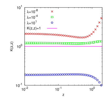
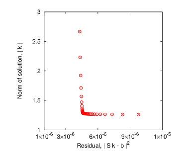
Figure 2: Results for the constant kernel, $K(m_{1},m_{2}=1$. The right panel shows the L-curve obtained by performing the minimisation Eq. (8) over a range of values of $\lambda$. The left panel shows the diagonal, $K(z,z)$, of the reconstructed kernels compared to the theoretical curve for values of $\lambda$ in the upper left, lower right and the “elbow” of the L-curve.

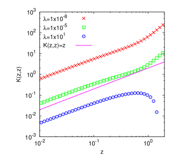
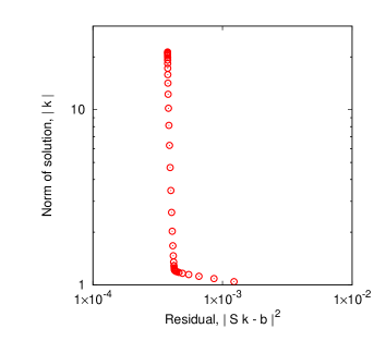
Figure 3: Results for the sum kernel, $K(m_{1},m_{2}=\frac{1}{2}(m_{1}+m_{2})$. The right panel shows the L-curve obtained by performing the minimisation Eq. (8) over a range of values of $\lambda$. The left panel shows the diagonal, $K(z,z)$, of the reconstructed kernels compared to the theoretical curve for values of $\lambda$ in the upper left, lower right and the “elbow” of the L-curve.

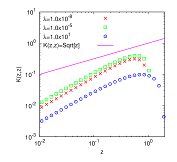
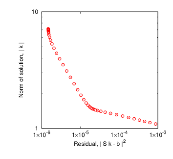
Figure 4: Results for the generalised sum kernel, $K(m_{1},m_{2}=\frac{1}{2}(\sqrt{m_{1}}+\sqrt{m_{2}})$. The right panel shows the L-curve obtained by performing the minimisation Eq. (8) over a range of values of $\lambda$. The left panel shows the diagonal, $K(z,z)$, of the reconstructed kernels compared to the theoretical curve for values of $\lambda$ in the upper left, lower right and the “elbow” of the L-curve.

The regularised least squares method described above was applied to several sets of data obtained by the numerical integration of Eq. (1) with monodisperse initial data with different model kernels. We used 40 discretisation points in the interval $z\in\left[0.01,2.0\right]$ and chose $p=3$ Laguerre polynomials in each direction. In each case, the data collapse and extraction of the scaling function was done using the method described in BS2001 and then fitted to a function of the form $C\,z^{\alpha-1}\,e^{-\beta\,z}$ as suggested in WR1992 . These fitted scaling functions were then used as the “observations”, $F(z)$, in the discretisation of Eq. (7).

Figs. 2 and 3 show some results of the regularised least squares for the constant kernel, $K(m_{1},m_{2})=1$, and the sum kernel, $K(m_{1},m_{2})=\frac{1}{2}(m_{1}+m_{2})$, respectively. These are good test cases to begin with since the solution of Eq. (1) with monodisperse initial data is known explicitly for each of these kernels allowing the numerical aspects of the calculation to be validated. The right panels of the figures show the L-curves obtained by performing the minimisation (8) over a range of values of $\lambda$. In both cases, a clear elbow is visible in the resulting curve indicating an appropriate range of values for $\lambda$. The left panel shows, for ease of visualisation, the diagonal, $K(m,m)$, of the kernels obtained by regularised least squares as a function of $m$ for different values of $\lambda$. The $\lambda$ curves shown correspond to values of $\lambda$ which are too big, too small and “just right” (meaning a value in the elbow of the L-curve). It is clear that the method does a reasonable job of extracting the basic shape of the kernel given the scaling function, $F(z)$. Surprisingly, we found that it was not necessary to explicitly enforce the positivity of $K(m_{1},m_{2})$ by constrainting the minimisation as was done in WR1992 . The method seemed to do equally well, and in some cases, better without these constraints. For the sum kernel, we did enforce the constraint that the kernel should vanish for particles of zero mass which seems physically reasonable - the results were less convincing without this constraint.

Fig. 4 shows the corresponding results for the generalised sum kernel $K(m_{1},m_{2})=\frac{1}{2}(\sqrt{m_{1}}+\sqrt{m_{2}})$. The results are clearly less convincing. This is probably related to the fact that this kernel cannot be expressed in terms of the Laguerre polynomials chosen to represent the kernel in Eq. (9). It is worth pointing out that the corresponding L-curve does not have a sharp elbow indicating that the method does not find a clear “best” value of $\lambda$. This seems to illustrate a point in favour of such methods - the fact that the L-curve does not have a sharp elbow provides an a-priori indication that the results of the minimisation should be treated with caution.

Empirical investigation suggest that the results for the generalised sum kernel can be improved by tinkering with the regularisation procedure. If, instead of, Eq. (8), we perform the minimisation

$$\min_{a} \lVert S\mathbf{k}-\mathbf{g}\rVert_{2}^{2}+\lambda\,w(\mathbf{k})$$ (10)

where

$$w(\mathbf{k}) =\sum_{i}\log(\lvert k_{i}\rvert+1)=\log\left[\prod_{i}(\lvert k_{i}\rvert+1)_{i}\right]$$ (11)

we found that the results were much better. This form for $w$ was found by experimentation. At present, this statement is at the level of empirical observation and requires further investigations.

V Discussion and outlook

We conclude, as several previous authors have done, that the inverse Smoluchowski problem is technically feasible and could potentially be developed into a useful tool for the study of droplet size distributions in clouds and other applications where the underlying microphysics is still incompletely understood. The results presented here indicate that the L-curve provides a useful complementary tool to the methods developed by Wright and Ramkrishna WR1992 to allow the regularisation parameter to be selected a-priori in situations where the collision kernel is not known from the outset. It is worth mentioning that the results presented in Figs. (2)-(4) do not give a good indication to the casual reader of the degree of numerical sensitivity required in tackling these problems. It became clear to us during these investigations that the ill-posedness of the inverse problem represented by Eq. (7) requires that great care be taken in interpreting the outputs of these methods. It is also clear that further research is required, even in the simple case of self-similar time evolution, in order to make the method more robust. Our results suggest that we should consider more general functional forms for the collision kernel than Eq. (9) in order to improve this robustness. This will probably not pose much difficulty since the analytic simplification obtained by the use of Laguerre polynomials in WR1992 is probably less important nowadays owing to the increased computational power which can be brought to bear on the computation of matrix elements by quadrature when closed analytic forms are not available.

In the long run, however, it is clear that it is necessary to free ourselves of the assumptions of homogeneity of the kernel and self-similarity of the cluster size distribution. Some strong progress in this direction has already been made recently by Onishi et al. OMTKK2011 who have been able to infer the relative importance of the turbulent and gravitational coagulation as a function of Reynolds number from direct numerical simulations of droplet-laden turbulence using inverse methods. Our approach differs slightly from this work in the sense that we would like, as far as possible, to learn the functional shape of the kernel from the data by allowing considerable freedom in the class of possible kernel functions. This approach would be more appropriate in situations when the underlying micro-physics is unknown or controversial.

References

- (1) G. L. Stephens, J. Climate 18, 237 (2005)
- (2) E. Bodenschatz, S. P. Malinowski, R. A. Shaw, and F. Stratmann, Science 327, 970 (2010)
- (3) H. Siebert, K. Lehmann, M. Wendisch, H. Franke, R. Maser, D. Schell, E. Wei Saw, and R. A. Shaw, Bull. Am. Meteorol. Soc. 87, 1727 (2006)
- (4) W. C. Reade and L. R. Collins, J. Fluid Mech. 415, 45 (2000)
- (5) L.-P. Wang, O. Ayala, B. Rosa, and G. W. Grabowski, New J. Phys. 10, 075013 (2008)
- (6) H. Wright and D. Ramkrishna, Comput. Chem. Eng. 16, 1019 (1992)
- (7) R. Onishi, K. Matsuda, K. Takahashi, K. Ryoichi, and S. Komori, Int. J. Multiphas. Flow 37, 125 (2011)
- (8) M. V. Smoluchowski, Z. Phys. Chem. 91, 129 (1917)
- (9) F. Leyvraz, Phys. Reports 383, 95 (Aug. 2003)
- (10) M. Ernst, in Fractals in Physics, edited by L. Pietronero and E. Tosatti (North Holland, Amsterdam, 1986) p. 289
- (11) M. Lee, Icarus 143, 74 (2000)
- (12) G. Falkovich, A. Fouxon, and M. G. Stepanov, Nature 419, 151 (2002)
- (13) P. van Dongen, J. Phys. A: Math. Gen. 20, 1889 (1987)
- (14) R. C. Ball, C. Connaughton, T. H. M. Stein, and O. Zaboronski, “Instantaneous gelation in the Smoluchowski coagulation equation revisited,” (2010), arXiv:1012.4431v1 [cond-mat.stat-mech]
- (15) P. C. Hansen, in Computational Inverse Problems in Electrocardiology, edited by P. Johnston (WIT Press, 2001) pp. 119–142
- (16) S. Bhattacharjee and F. Seno, J. Phys. A–Math. Gen. 34, 6375 (2001)