Motifs emerge from function in model gene regulatory networks

Abstract

Gene regulatory networks arise in all living cells, allowing the control of gene expression patterns. The study of their topology has revealed that certain subgraphs of interactions or “motifs” appear at anomalously high frequencies. We ask here whether this phenomenon may emerge because of the functions carried out by these networks. Given a framework for describing regulatory interactions and dynamics, we consider in the space of all regulatory networks those that have a prescribed function. Monte Carlo sampling is then used to determine how these functional networks lead to specific motif statistics in the interactions. In the case where the regulatory networks are constrained to exhibit multi-stability, we find a high frequency of gene pairs that are mutually inhibitory and self-activating. In contrast, networks constrained to have periodic gene expression patterns (mimicking for instance the cell cycle) have a high frequency of bifan-like motifs involving four genes with at least one activating and one inhibitory interaction.

I Introduction

Both natural and artificial networks have unexpected properties that may find their origin in the way they were constructed. However, another possibility, in particular in the context of biological networks, is that constraints associated with network functionality are the main determinants of these unexpected properties. We focus here on gene regulatory networks (GRN), the set of interactions between genes as well as the rules for expression dynamics that allow all living cells to control gene their expression patterns. In the last decade, gene interactions have been measured, modified, engineered, etc., and so quite a lot is known about how any given gene can affect another’s expression. Furthermore, small gene networks have been designed to implement simple functions in vivo Elowitz and Leibler (2000); Gardner et al. (2000), and much larger sets of interactions have been reconstructed in a number of organisms Herrgard et al. (2004); Salgado et al. (2006); Hu et al. (2007). From these large networks it has been possible to show that several “motifs” – subgraphs with given interactions – arise far more often than might be expected Shen-Orr et al. (2002); Ma et al. (2004); Lee et al. (2002); Zhu et al. (2008). One of the most studied motif is the so called Feed Forward Loop or FFL, a graph based on three genes where the first regulates the second, and both the first and the second regulate the third. Another example is the bifan motif in which 2 genes control two others. Biological functions have been proposed for these motifs Mangan and Alon (2003); Camas and Poyatos (2008) which give them some meaning, but one may ask whether other motifs could perform the same functions and what level of enrichment might be expected if function were the sole cause of motif over-representation. Unfortunately, the functions of GRN and the constraints they must satisfy (e.g., kinetic response characteristics or robustness to noise) are still poorly understood, so such questions cannot be addressed in a truly realistic framework. Instead, we will (i) work within a plausible model of transcriptional regulation, (ii) impose functional constraints on the patterns of gene expression, (iii) determine which motifs emerge when considering the space of all possible functional GRN. This particular task is related to previous work that used genetic algorithms or simulated annealing to design genetic networks having given functional properties François and Hakim (2004); François et al. (2007); Rodrigo et al. (2007). Those studies found that the optimization procedures indeed led to particular architectures. Our approach differs by not relying on a design procedure: we want to get away from any dependence on the optimization algorithm and see how functionality on its own constrains the possible architectures. In this framework, two types of constraints will be applied: we will impose either a set of steady-state expression patterns, or a time periodic pattern of expression motivated by previous studies of cell cycling. Interestingly, we find very different motifs for these two cases; in Alon’s Alon (2007) terminology, bifan, diamond and four point cycle motifs appear only in the second case.

Our model of transcriptional regulation is simple enough to be used for illustration and, hopefully, for identification of the generic features of genetic networks, but at the same time is rooted in bio-physical reality to avoid ad-hoc assumptions. It significantly extends the framework of ref. Burda et al. (2010), in particular by allowing for inhibitory interactions. We begin by describing our model and then show its properties, in particular the kinds of motifs that emerge from the functional constraints imposed on the networks.

II The model

II.1 Transcription factor binding

We start with $N$ genes coding for transcription factors that may influence each other’s expression. To keep the model as realistic as possible, we include the known biophysical determinants of transcriptional control. In particular, the binding of a transcription factor (TF) to a site is described thermodynamically von Hippel and Berg (1986); Berg and von Hippel (1987); Gerland et al. (2002) and depends on the mismatch of two character strings of length $L$, one for the TF and one for the binding site. Up to an additive constant, the associated free energy in units of $k_{B}T$ is taken to be $\varepsilon d_{ij}$ where $d_{ij}$ is the number of mismatches, $T$ is the temperature and $k_{B}$ is Boltzmann’s constant. The parameter $\varepsilon$ is a penalty per mismatch which has been measured experimentally to be between one and three if each base pair of the DNA is represented by one character Sarai and Takeda (1989); Stormo and Fields (1998); Bulyk et al. (2002). Also, by comparing to the typical number of base pairs found for experimentally studied binding sites, one has $10\leq L\leq 15$. For all the work presented here, we use $\varepsilon=2$ and $L=12$, but we have checked that our conclusions are not specific to these values.

We shall define the “interaction strength” $W_{ij}$ from gene $j$ to gene $i$ via the Boltzmann factor

$$W_{ij}=e^{-\varepsilon d_{ij}}/Z$$ (1)

where $Z$ is normalization (a partition function). If there were just one transcription factor molecule of type $j$, $W_{ij}$ would be the probability to find that molecule bound in gene $i$’s regulatory region. Gerland et al. Gerland et al. (2002) have shown that in practice $Z$ in Eq. (1) is close to 1 and that the probability of finding any given TF molecule bound rather than unbound is quite low.

Figure 1: Each gene’s regulatory region contains $N$ binding sites, one for each of the $N$ transcription factors produced by the $N$ genes. The probability of occupation (POCC Granek and Clark (2005)) of the regulatory region determines the average transcription rate of the gene $i$ under consideration.

For simplicity, and to prevent different TFs from accessing a same site, we use a standardized form of regulatory region for each gene. This situation is illustrated in Fig. 1 for gene $i$ which produces the transcription factor $TF_{i}$. The regulatory region of each gene has $N$ binding sites, one dedicated to each of the $N$ different TF types. Suppose, that there are $n_{j}$ TF molecules of type $j$ that can bind to the site $j$ in gene $i$’s regulatory region; given that this site can be occupied by only one TF molecule at a time, it is necessary to take into account possible competition effects between all molecules $n_{j}$ of type $TF_{j}$. Using the fact that $Z$ in Eq. (1) is close to 1, it is possible to approximate the occupation probability of the binding site by Gerland et al. (2002):

$$P_{ij}=\frac{1}{1+1/(n_{j}W_{ij})}\;.$$ (2)

As emphasized in Burda et al. (2010), $P_{ij}$ depends strongly on $d_{ij}$ and is appreciable only when the mismatch is small, which is an a priori unprobable event imposed in functional genotypes by the selection pressure.

II.2 Transcriptional control

Again for pedagogical reasons, we shall consider that all genes have the same maximal transcription rate; denoting by $n$ the associated maximum number of TF molecules in the system of a given type, we shall set $n_{j}=S_{j}n$ where $S_{j}$ is then the current (normalized) level of transcription for gene $j$, ranging between 0 and 1. Experimentally, $n$ is known to range from of order unity to many thousands Golding et al. (2005); Becskei et al. (2004); Elf et al. (2007). Here we shall use $n=1000$, but again we have checked that using values ten times smaller or larger does not change our conclusions.

The expression $S_{i}$ of gene $i$ will vary with the presence of transcription factors bound in its regulatory region, but present knowledge does not provide us with quantitative information on this dependence. Much past modeling work Kauffman (1993); Wagner (1996); Bornholdt and Rohlf (2000); Li et al. (2004); Azevedo et al. (2006) has dealt with this obstacle by considering that each occupied binding site provides an activating or inhibitory signal and that all signals are then added and compared to a threshold: below (respectively above) this threshold, transcription is off (respectively on). However, more recent experimental work and associated modeling Segal and Widom (2002); Giorgetti et al. (2010) suggests that transcription rates in vivo can exhibit graded responses. This result is not surprising given that transcription factors are sometimes bound and sometimes not, so any average transcription rate has no reason to be binary. Our work thus follows Segal and Widom (2002); Giorgetti et al. (2010); Burda et al. (2010) by considering continuous transcription rates determined by the probabilities that binding sites are occupied.

Consider first the case where all $N$ transcription factors affect gene $i$ as activators. If at least one of the binding sites is occupied by its TF, we consider that the gene will be transcribed; this choice corresponds to having the transcription rate be proportional to the Probability of OCCupation or “POCC” Granek and Clark (2005) of the regulatory region. Calling $P_{i}$ this probability, we have

$$P_{i}=\sum_{k=1}\sum_{[j_{1},...,j_{k}]}P_{i}^{(k,N-k)}(j_{1},...,j_{k},\bar{j}_{k+1},...,\bar{j}_{N})$$ (3)

where $j_{l}$ ($\bar{j}_{l})$ is the label of an occupied (unoccupied) binding site and $[j_{1},...,j_{k}]$ stands for a combination of $k$ out of $N$ gene labels. Assume now that the bindings arise independently (no cooperativity), i.e. that the probabilities in the sum factorize into a product of terms $P_{i}^{(1,0)}(j)$ (or $P_{i}^{(0,1)}(j)$). Replacing $P_{i}^{(1,0)}(j)$ by $P_{ij}$ defined in Eq. 2 we write

$$P_{i}^{(k)}(j_{1},...,j_{k},\bar{j}_{k+1},...,\bar{j}_{N})=\prod_{j}P_{ij}\times\prod_{j^{\prime}}(1-P_{ij^{\prime}})$$ (4)

where $j$ runs over indices for which there is binding and $j^{\prime}$ runs over the other indices. Now, the sum over $k$ in Eq. 3 can be explicitly performed. In addition, we identify up to an overall scale the transcription rate with the probability of occupancy $P_{i}$. Considering that protein content is proportional to transcription rate (at least in the steady state), we set $S_{i}$ – the mean normalized expression level of gene $i$ – equal to $P_{i}$. One finally gets

$$S_{i}=1-\prod_{j}(1-P_{ij})$$ (5)

which is the basic equation of the “mean field” model of ref. Burda et al. (2010). The neglect of fluctuations and the corresponding limitations were already explained there. Note that if the $P_{ij}$ are small, transcription is additive in these variables, while in the binary limit where $P_{ij}$ is 0 or 1, $S_{i}$ corresponds to the logic of transcription being “on” if and only if at least one of the binding sites is occupied, as expected from the use of the POCC.

Our treatment of inhibitory interactions (due to repressors) is new and is motivated by a number of known cases where the binding of a TF acts as a veto. One way this can happen is if the presence of the TF makes the DNA form a loop that conceals the other binding sites. Another mechanism for vetoing transcription is simply for the bound TF to block the advance of the polymerase. Within our framework, transcription proceeds as in Eq. 5, in the absence of such repressors bound to their sites, but as soon as any of the inhibitory sites are bound, transcription is turned off. Assuming cooperative effects are absent as before, and repeating for repressors the argument just used for activators, we are led to modify Eq. 5 to

$$S_{i}=[1-\prod_{j}(1-P_{ij})]\prod_{j^{\prime}}(1-P_{ij^{\prime}})$$ (6)

where $j$ runs over activating interactions and $j^{\prime}$ over inhibitory interactions.

The transcriptional dynamics is then defined as follows. Just like in many other modeling frameworks, we take time to be discrete Kauffman (1993); Wagner (1996); Bornholdt and Rohlf (2000); Li et al. (2004); Azevedo et al. (2006); at each time step we first update the $P_{ij}$ in Eq. 2 (using $n_{j}=nS_{j}$) and then update the $S_{i}$ in Eq. 6. These updates are deterministic, and in general the system goes towards a fixed point (corresponding to steady-state expression levels) or towards a cycle (corresponding to periodic behavior of the expressions in time).

By neglecting cooperative effects, we obtain a toy model where the only parameters are those determining the binding probabilities implicit in Eq. 2 and these are subject to experimental constraints. Incorporating cooperative effects could lead to a more realistic model but at the cost of more parameters. For instance, one could replace in Eq. 4 the equality by a proportionality. Such an assumption often appears in the literature: using the stationary limit of appropriate kinetic equations, one argues that the concentration of a molecular complex is proportional to the product of concentrations of the constituents. Here, because of the reparametrization symmetry of the dynamics, the proportionality constant can only depend on $k$. One could then truncate the sum over $k$, say at $k=3$, to avoid too many free parameters, a situation that arises in a number of genetic network reverse engineering attempts. Such a model deserves study, but this is beyond the scope of the present work.

II.3 Genotypes and Phenotypes

As previously mentioned, the TFs and their binding sites are associated with character strings. We are interested in the space of all GRN, which means here all possible character strings. However, it is easy to see that all choices of TF character strings are equivalent, so we can fix them without any loss of generality. (Biologically, it is known that TF and most protein coding genes are far more conserved than the TF binding sites. See ref. Burda et al. (2010) for a discussion of this point.) Any given GRN is then completely specified by the $N^{2}$ character strings of its binding sites and by the specification of the activating or inhibiting nature of each interaction. Since DNA bases come in four types, A,C,G,T, we use an alphabet of four characters for our strings. This set of strings is referred to as the “genotype” of the GRN. Clearly the most relevant quantities in a genotype are the mismatches $d_{ij}$ of these $N^{2}$ strings to their TF string. A genotype can then usefully be represented by this $N$ by $N$ matrix of mismatches or by the corresponding matrix of interaction strengths $W_{ij}$, plus the sign (activating vs. inhibitory) associated with each of these interactions.

At any time step $t$, the pattern of mean gene expression can be represented by the vector ${\mathbf{S}}(t)=\{S_{j}(t)\}_{j=1,\ldots N}$. We shall consider two classes of functions to be imposed on our GRN. The first is motivated by cell types in multi-cellular organisms: we want the GRN to be able to have steady state expression vectors that are very close to 2, 3, or more target patterns, each associated with a different tissue. Note that some such patterns involving a dozen or so genes have been inferred in various organisms Espinosa-Soto et al. (2004); Chickarmane and Peterson (2008). The second kind of function we shall impose is for the vector to follow tightly and step by step a sequence of patterns that forms a target cycle. Such cases of cycling GRN have been studied previously within threshold and boolean models Li et al. (2004); Davidich and Bornholdt (2008).

For each type of functional constraint imposed, we refer to the “phenotype” of the GRN as (i) the different steady-state expression vectors for the first case; (ii) the cyclic pattern of expression vectors for the second case. Given a GRN genotype, determining its phenotype is straightforward in practice. In the first case where we have given target expression patterns, we start in these target vectors and we see whether we converge to a nearby fixed point under iteration of the transcriptional dynamics. (In contrast, in our previous work, we had considered initial states that were unrelated to the target vector.) In the second case, we start with one of the patterns in the target cycle and see whether the trajectory under iterations stays close to that cycle. For the steady state behavior, we shall impose 2, 3, or more vectors that consist of $N/2$ levels at 0 and $N/2$ at 1, and furthermore that are taken to be orthogonal (for the 0/1 coding for $S_{i}$ this means that the scalar product of two vectors is $N/4$). Setting $N=16$ (the choice of $N$ is not important as long as it has a moderate value, but we have not explored what happens at large $N$), we define four mutually orthogonal targets as follows, a direct generalization of that of ref. Burda et al. (2010):

1 1 1 1 1 1 1 1 0 0 0 0 0 0 0 0
1 1 1 1 0 0 0 0 1 1 1 1 0 0 0 0
1 1 0 0 1 1 0 0 1 1 0 0 1 1 0 0
1 0 1 0 1 0 1 0 1 0 1 0 1 0 1 0
This choice is motivated by the fact that at large $N$, random binary vectors are typically nearly orthogonal. The symmetries of the model are relevant for studying it, but with any interesting choice of vectors, most of the symmetries are broken. Note that since one can transform these vectors into each other by index permutation, the basins of attraction leading to these targets are on average of equal size.

For the case where one enforces a target cycle, we shall use the toy sequence where the genes are taken to lie on a ring, and the cycle consists in having the “on” genes shift to the right at each time step:

1 1 1 1 1 1 1 1 0 0 0 0 0 0 0 0
0 0 1 1 1 1 1 1 1 1 0 0 0 0 0 0
0 0 0 0 1 1 1 1 1 1 1 1 0 0 0 0
0 0 0 0 0 0 1 1 1 1 1 1 1 1 0 0
0 0 0 0 0 0 0 0 1 1 1 1 1 1 1 1
1 1 0 0 0 0 0 0 0 0 1 1 1 1 1 1
1 1 1 1 0 0 0 0 0 0 0 0 1 1 1 1
1 1 1 1 1 1 0 0 0 0 0 0 0 0 1 1
1 1 1 1 1 1 1 1 0 0 0 0 0 0 0 0
This is reminiscent of the cycle studied by Li et al. Li et al. (2004) for the yeast cell cycle. We have also considered a cycle where the shift is not by two, but by 1 or 3 steps. The results are nearly the same in all these cases.

To quantify the deviations from the ideal target behavior, we first check whether we have steady-state behavior (in the first case) or cyclic behavior (in the second). For each target vector ${\mathbf{S}^{(target)}}$, we define its distance to the associated GRN specific expression vector ${\mathbf{S}}$ via:

$$D({\mathbf{S}},{\mathbf{S}^{(target)}})=\sum_{i}\mid S_{i}-S_{i}^{(target)}\mid\;.$$ (7)

By summing all these distances, one for each target (each steady state in the first case, and each expression vector of the periodic cycle in the second), we obtain what we refer to as the “total” distance $D_{T}$ for that GRN. The resulting measure of “fidelity” to the imposed function can be turned into a kind of fitness via

$$F(GRN)=\exp{(-fD_{T})}$$ (8)

where $f$ acts as a control parameter allowing one to be more or less stringent on the fidelity. We thus consider the set of all GRN and apply the relative weight $F(GRN)$ to each; this then provides an ensemble for the GRN, and by adjusting $f$ we can focus on those GRN that are the most functional. For specificity, we shall work with $f=20$, but our results depend only very weakly on this choice provided $f$ is in the range 10 to 100.

II.4 MCMC sampling

To sample our ensemble of constrained genotypes, we apply a Monte Carlo Markov Chain (MCMC) using the Metropolis rule. This computer algorithm produces a (biased) random walk in the fitness landscape that visits at long times the different genotypes according to their fitness as given in Eq. 8; the sampling thus focuses on genotypes having high fidelity to the imposed functions. In detail, we perform random mutations of the binding sites. This produces changes to the edge weights and thus to the genotypes. (Technically, it would be possible to work at the level of edge weights alone, but it would make explanations of the MCMC far more delicate.) A sweep is defined as $LN^{2}$ successively attempted changes of the genotype (a random mutation of one coding letter and, independently, a random switch of the sign of one of the TF-DNA interactions). Each such change is accepted or rejected by the Metropolis algorithm. We always make a hot start, using as input a completely random GRN. After some time, as in ref. Burda et al. (2010), we produce a GRN sufficiently close to the target (see Fig. 2), and we use this to start

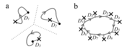
Figure 2: A schematic representation of our MCMC process. (a) Steady state behavior and $n=3$: crosses (heavy dots) stand for the target (fixed point) states, while the line is the system’s trajectory. The ”total” distance entering the Metropolis test is $D_{T}=D_{1}+D_{2}+D_{3}$. (b) Similar as before, but for a cycle. Grey dots stand for successive states obtained by iterating Eq. 6. Here $D_{T}=D_{1}+\dots+D_{8}$.

the production run of the MCMC. Thereafter, we iterate sweeps, recording successive GRNs. Unfortunately, the simulation requires a lot of computation time, especially for $L=12$, where small mismatches become very unprobable. Therefore, we resort to the following modified procedure. We first set $L=8$ and generate an MCMC sampling, recording genotypes every 100 sweeps. Since our dynamics depends on mismatches and not on the value of $L$, these recorded GRNs are also fit at $L=12$, except that the distribution of the magnitudes of the mismatches is wrong. Hence we set $L=12$ and upgrade our GRNs, obtaining in this way a sample of fairly independent genotypes in a reasonable time.

II.5 Essential interactions and the essential network

As already mentioned, genotypes can be represented by the $N$ by $N$ matrix of entries $W_{ij}$s along with the $N^{2}$ signs specifying the activating vs. inhibitory types of each interaction. These $W_{ij}$ are never zero (cf. Eq. 1), so we cannot say that an interaction is completely absent. Nevertheless, one may expect some interactions to be more important than others, for instance when the $W_{ij}$s are larger than average. An arbitrary cut-off could be introduced for separating small and large values, but it is better to base such a classification on functionality. We thus consider what happens when an interaction $W_{ij}$ is removed by setting it to zero. Starting with one of the genotypes generated by our MCMC (and thus typically satisfying well the soft functional constraints), we determine the change in fitness produced by setting $W_{ij}$ to zero: if the change is rejected by Metropolis in five successive attempts, we say that this interaction is essential, motivated by the corresponding biological definition (a very similar result is obtained by defining the essentiality as the sensitivity to a single deleterious mutation; since the definition of essentiality involves the Metropolis test, a random event, one sometimes finds false essentials, however this is a very weak effect). This definition leads to a summary description of a genotype via a list of pairs $(i,j)$ specifying the essential interactions as well as their nature (activating or inhibitory). This can then be represented by a directed graph, with + signs on the edges that are activating and - signs on the edges that are inhibitory. Hereafter we refer to this oriented and signed graph as the essential network of the genotype; note that no information on the weights of the interactions is attached to this network representation.

III Results

III.1 Abundance of functional GRN

The space of all GRN is finite in our framework since each genotype can be specified by $N^{2}$ character strings of length $L$ and the signs of the associated interactions. In this space we impose the soft constraint that a GRN implements a function specified by a certain target expression behavior. Is such a constraint very stringent? To find out, we have generated millions of random genotypes and find that none of them have good expression behavior: their fitness is orders of magnitude lower than what we obtain from our MCMC sampling. Thus, as in other gene network models Ciliberti et al. (2007), by focusing on “functional” GRN, we are considering an extremely small subset of all GRN; these very rare GRN may thus very well be atypical in many of their properties. Nevertheless, as long as the number of constraints is not too high (the number of steady states or length of the cycle cannot grow indefinitely), the number of high fitness genotypes is huge. Indeed, our MCMC is able to produce essentially as many different GRN as we want even though the ensemble of interest is only an infinitesimal part of the whole; this feature arises also in other genotype to phenotype mapping models such as RNA neutral networks Wagner (2005).

We have also checked that the basin of attraction of a target phenotype represents a large fraction of all possible initial phenotypes, so that the fact of performing the imposed function is not merely a dynamical accident. These basins constitute approximately 99.8(9)%, 52.9(9)% and 49.6(8)% of the whole space for $n=$ 2, 3 and 4 respectively. As already explained, with our choice of target phenotypes, the basins associated with individual targets are equal (after averaging over functional GRNs).

III.2 Functional GRN have sparse essential networks

A question that comes to mind is whether essential interactions are frequent or not. Consider first the case of the multi-stability phenotype where we impose 1, 2, 3, … steady states. In previous work Burda et al. (2010) on a simpler model allowing no inhibitory interactions, we found that imposing a single steady state led to sparse essential interactions, with the great majority of genotypes having just one essential interaction $(i,j)$ for each gene $i$. In the present model allowing for inhibitory interactions, this property remains true (see Table 1, where some of our results are summarized). As we impose more steady states, the mean number of essential interactions grows; again each gene $i$ will typically have just a few essential interactions (and almost never none), with a mean of $1.2$, $1.5$, $1.9$ for 2, 3, and 4 steady states at $N=16$. Furthermore, these means are quite stable as one increases $N$, so the essential networks of our functional genotypes form sparse graphs. The mean degree of these networks is insensitive to $N$, but grows when the number of constraints imposed on the GRN is increased.

Table 1: A sample of results of our simulations. nFP stands for phenotypes with $n$ fixed points. The robustness is defined as the frequency of genotypes surviving a random mutation according to the Metropolis rule. Notice that it is fairly well reproduced by $1-n/2N$, a result generalizing an analogous result of ref. Burda et al. (2010). The distance to the target is the distance entering the fitness. It is nearly constant when divided by the number of target phenotypes. Further division by the number of active genes in a phenotype, i.e. $N/2$, yields approximately 6%, which measures the average deviation of their activity from the maximum $S_{i}=1$.

observable	2FP	3FP	4FP	cycle
$\langle\mbox{\rm\#essentials}\rangle$	14.70(1)	21.08(2)	29.39(1)	23.42(1)
$\langle\mbox{\rm\#repressors}\rangle$	2.500(12)	6.38(2)	10.11(1)	7.38(1)
$\langle\mbox{\rm robustness}\rangle$	0.9494(2)	0.9259(2)	0.8998(3)	0.9099(3)
$\langle\mbox{\rm dist2target}\rangle$	0.966(3)	1.390(4)	1.961(4)	3.583(4)

The situation is similar when a cyclic phenotype is imposed: only a small fraction of the interactions turn out to be essential. For the toy cases where the genes are on a circle and the cycle shifts the “on” genes by steps to the right, we find again that the essential networks associated with the genotypes of our MCMC ensemble are sparse, and that the connectivity hardly changes as one increases the number of genes.

There is a simple explanation for this sparseness: at the level of the GRN, introducing an additional essential interaction generally means increasing a $W_{ij}$. That has a high entropy cost as can be seen from the mismatches (there are few strings that have a low mismatch, and many that have a high mismatch). On the contrary, if one were to consider a Boolean model at the level of the essential network (to go from genotypes to phenotypes) and ignoring the molecular basis of the interactions, one would inevitably have far more functional graphs with dense interactions than with sparse interactions; sparseness would then have to be enforced in an ad-hoc way since biological networks are indeed sparse experimentally Thieffry et al. (1998); Balazsi et al. (2008).

III.3 Functional essential networks have parsimonious inhibitory interactions

Are inhibitory interactions as frequent as activating ones? The answer to this question depends on the interactions considered. Indeed, even though the genotypes generated by the MCMC sampling have functional constraints, the many small $W_{ij}$ arising in genotypes have hardly any effect on the phenotype; their sign will thus be random, and in effect they act like noise. If instead we focus on the larger $W_{ij}$, the functional constraints are likely to bias the sign in favor of activating interactions. To avoid an arbitrary definition of large weights, we again use the notion of essentiality because of its link with phenotypes. For the essential networks produced from the GRN of our MCMC with the constraint of 2 to 4 steady states, we find that the great majority of the interactions are activating, cf. Table 1 (these numbers are not sensitive to $N$). These results are not surprizing: increasing the number of constraints forces the connections to be more complex and to make greater use of inhibitory interactions. In the toy cases of genes on a ring, we also see this general picture and find that the number of both activating and inhibitory essential interactions grows linearly with $N$.

III.4 Abundance of functional essential networks

Another question of interest concerns the number of distinct functional essential networks (the number of distinct GRNs is of little interest, being trivially enormous since all inessential interactions can be changed at will without affecting the phenotype). It is wise to first find the essential networks that are in a sense representative for a group of GRNs, in other words to perform a cluster analysis of the sample of essential networks at our disposal. Let the numbers of such networks be $M$ and define a distance between a pair of them, for example

$$\mbox{\rm Distance}(A,B)=\sum_{ij}(A_{ij}-B_{ij})^{2}$$ (9)

where $A_{ij}$ (viz. $B_{ij}$) is $\pm 1$ for essential interactions and 0 otherwise. Our question can now be reformulated more precisely: does the number of clusters, considered a proxy for the number of representative essential networks, saturate at some moderate value as $M$ or not? (It must saturate somewhere, of course, but that may be at very large values.) To answer this, it is most convenient to use the modern affinity propagation algorithm Frey and Dueck (2007), where the number of clusters is not preassigned but is determined by the algorithm; the code can be downloaded from www.psi.toronto.edu/index.php?q=affinity propagation. As an illustration, for 4 fixed points we find that the number of clusters grows at large $M$ roughly like $M^{2/3}$ (with a prefactor of the order of 0.3) and shows no sign of saturation up to at least $M=4000$. Other values of $n$ lead to similar results, but some care is necessary in interpreting these trends at $n=2$ and $3$. Indeed, it turns out that for these values of $n$ many clusters, distinct according to eq. (9), have essentially the same topology and differ merely by the labeling of nodes (this reflects symmetries in our choice of the target phenotypes). In contrast, for $n=4$ the clusters are genuinely different. To get more insight into this problem, we have carried out a complementary investigation, counting the number of distinct topologies (instead of using the clustering algorithm). This is very tedious and our account of the network reparametrizations was only partial. With this proviso, it appears that the number of distinct topologies again increases like a power of M, however now the exponent increases with $n$ (approximately from 0.69 for for $n=2$ to $0.97$ for $n=4$).

Beyond clusters, we can also ask which essential network topologies are the most frequent. In Fig. 3 we display the most frequent topology when imposing $n=2$ and 4 fixed points. As $n$ increases, the connections becomes more complex as expected; in particular at small $n$ much of the topology is tree-like; to a large extent, this reflects the sparseness and parsimony of these essential networks. Note that our GRN are connected by a succession of point mutations. This shows that the same function can be performed by a very large number of distinct networks, a feature also found in other models of gene networks Ciliberti et al. (2007), but here we show that many different topologies arise too.

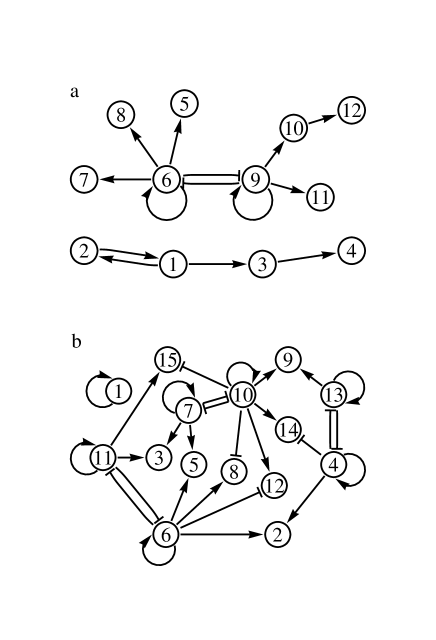
Figure 3: The most common essential network topologies when $n$ steady-state expression patterns are imposed. In each case, we see the presence of the motif with two mutually inhibiting and self-activating genes. Interactions shown are essential, and those genes whose target expression is the same in all the steady states are omitted since they provide no information. (Data for $N=16$; sub-figures a and b are for $n=2$ and $4$. These topologies arise for over 20% and less than 1% of the networks, respectively).

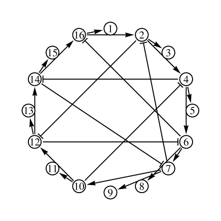
Figure 4: The most common essential network topology when one imposes a particular cyclic expression pattern. That pattern corresponds to a group of active genes that shifts clockwise at each step. One sees very clearly the activating interactions acting downstream and the inhibitory interactions acting upstream. (Data for $N=16$; this topology arises for over $15\%$ of the networks.)

III.5 Functionality leads to motif selection

Working with the full description of genotypes is cumbersome and difficult, whereas focusing just on essential networks provides a great deal of intuition, in particular for what features are relevant for functionality. The price to pay for this simplicity is some loss of information; for example, two interactions separately may be non-essential but nevertheless if one removes both of them the network’s functionality may be lost.

To obtain insights into network structure, one can search for network motifs; this has become very popular in recent years, to a large extent through the effort of U. Alon and collaborators Milo et al. (2002); Alon (2007) (see also the web page www.weizmann.ac.il/mcb/UriAlon/). The fact that a complex network can be constructed from small standard sub-elements is by itself not surprising. For example, this property is at the root of electronics and is based on the mathematical structure of logical functions. However, the fact that nature also uses this strategy is not obvious, and that some motifs and not others are employed in different network functions is even less obvious. This presence of motifs is revealed though from the detailed studies of (rather rare, for obvious reasons) biological networks reconstructed from data, and it has been partly explained by arguments borrowed from communication systems techniques. This brings us to inquire what happens in a model where the same dynamics is always at work, and where thousands of networks can be generated for several network functions: will the same motifs emerge when the functionality constraints are modified, or will the motifs change with the functions implemented by the networks.

To answer the previous question, we determine the motifs in our different ensembles. The web page mentioned above offers a software for motif search; it is not quite adapted to our needs, since it does not distinguish between activators and repressors, and does not accept self-interactions. However, it was helpful in this work, enabling us to single out the relevant motif topologies (when a topology is irrelevant, it is also so when more detailed distinctions are introduced). Furthermore, we used it to test our own codes for motif extraction. The results presented here concern the most prominent motifs; others have frequencies that are either very small or at least roughly of the order of the expectation for a randomized network. We discard motifs with leaves (degree-one nodes), which are somewhat trivial. We keep only motifs that are not a subgraph of a larger motif with the same number of nodes. However, our motifs can partly overlap. The randomization used is that proposed by Maslov and Sneppen Maslov and Sneppen (2002): the links are interchanged, so that both the in- and out-degrees of network nodes remain unchanged. Our results are summarized in Table 2 and the motifs are listed and defined in Fig. 5.

Table 2: Most important motifs. nFP means “n fixed points phenotype”. Cycle refers to our 8-step cycle. We typically used 1000 GRNs in our motif search.

motif	2FP	3FP	4FP	cycle
motif a: model	0.706(16)	2.358(39)	2.984(4)	0.000
randomized	0.002(1)	0.002(1)	0.002(2)	0.000
motif b: model	0.000	0.000	0.000	5.451(41)
randomized	0.001(1)	0.008(3)	0.071(9)	0.023(5)
motif c: model	0.000	0.000	0.000	5.170(40)
randomized	0.000	0.008(3)	0.078(9)	0.029(1)
motif d: model	0.000	0.000	0.000	4.533(42)
randomized	0.000	0.014(4)	0.0180(6)	0.030(7)
motif e: model	0.000	0.000	0.000	6.676(22)
randomized	0.017(4)	0.102(16)	0.057(8)	0.173(14)
motif f:	0.000	0.000	0.000	2.296(29)
randomized	0.000	0.001(1)	0.050(6)	0.003(2)

Figure 5: The most prominent motifs found for our two classes of functional constraints. Case of multi-stability (more than one steady-state): (a) two mutually inhibiting and self-activating genes. Case of expression targets that are cyclic in time: (b,c) diamond motif, (d,e) four-node loop, (f) bifan.

We see right away a very strong dichotomy: the motifs are very different for our two classes of functions (imposing multi-stability vs. cycling). In the case of multi-stability, one single motif stands out as being extremely important: two genes that are mutually inhibitory and which are self-activating. Clearly such a pair of genes can act as a switch that will then influence downstream genes according to the expression pattern that is required for the considered fixed point. When dealing with more than two target fixed points, additional such motifs should be necessary. That is indeed what we saw in Fig. 3 which displayed the most represented essential network (ignoring permutations of indices) for 2 and 4 imposed fixed points. Interestingly, the same trend also emerges for the less frequent essential networks (data not shown). Roughly, the networks display a core of central genes that belong to a motif of type “a” (using the nomenclature shown in Fig. 5) and these genes then influence other genes by a simple downstream effect along the associated tree-like graph of activating interactions.

Now when we look at the motifs present when imposing cyclic expression targets, the previous motif is absent and instead we have several four gene motifs that are strongly over-represented. Motif “f” is the bifan in the nomenclature of Alon; the others generally involve a regulatory loop, and in particular motifs “d” and “e” are “frustrated” in that they have loops with an odd number of inhibitory interactions. None of these were over-represented in the networks satisfying multi-stability. Their presence can be understood by looking at the dominant essential networks such as in Fig. 4. Note that these motifs are analogous to the ones driving repressilators Barkai and Leibler (2000) but they involve more genes and do not provide oscillatory behavior on their own, their function requires the presence of the other genes that are not included in the motif construction.

IV Discussion and conclusions

The central question tackled by the present work is whether the emergence of motifs in gene regulatory networks can be due to functional constraints. Given the uncertainties in how real genetic networks function, we have taken a modeling route and have addressed this question in silico. Our model incorporates known molecular mechanisms for the description of genetic interactions, and in fact the only parameters in our model come from parametrizing the affinities of transcription factors to their binding sites. Furthermore, in contrast to most other gene regulatory network modelings, the associated interactions are never completely absent; they can be important or unimportant for the functionality of the network, a notion we characterized by the essentiality of interactions. Finally, the expression level of each gene follows dynamics allowing for continuous values; this additional complexity compared to using digital “on-off” expression levels forces one to consider functionality as a soft constraint, imposing expression levels to be “sufficiently” close to target patterns. Network functionality is then quantified via a fitness measure. Such a framework provides a close parallel with thermodynamic ensembles; all questions are then necessarily posed in a probabilistic framework where each network arises with a probability proportional to its fitness. In practice, we explore the corresponding ensemble of genetic networks numerically, using Monte Carlo Markov Chain.

Two types of gene network functionalities have been studied. The first is motivated by the different cell types in multi-cellular organisms and is implemented by constraining the genes in the networks to have steady-state expression levels close to given target levels; in effect, the transcriptional dynamics of the networks must allow for multi-stability, that is multiple fixed points of the expression dynamics. The second type of functional constraint considered is motivated by previous work on the cell cycle; we implemented such a constraint by forcing the networks to have their expression levels follow a given cyclic pattern in time. Thus instead of fixed points, in this case we ask for a periodic behavior of the dynamics. In both cases, we found characteristic features shared with other models of living systems Wagner (2005) as follows. (1) The constraints imposed are extremely stringent as can be seen from the fact that in practice they are never satisfied by randomly generated networks. (2) Although the fraction of networks of interest is tiny, the number of networks satisfying the constraints is astronomical as revealed by our Monte Carlo Markov Chain sampling.

Of interest is the structure of these presumably atypical networks. Particular architectures are known to arise when performing genetic network design via optimization algorithms François and Hakim (2004); François et al. (2007); Rodrigo et al. (2007). Is this property a bias of these algorithms or does it reflect an underlying constraint imposed by network function? It is difficult to tackle this question head-on except in very small systems; there one can explore all possible values for the model’s parameters Guantes and Poyatos (2008) and see the functional consequences. Since motifs can involve three or even more genes inside a larger network, a different approach is necessary for moderate and large networks. The most adapted tool is based on Monte Carlo Markov chains and so we have applied this approach to our systems with up to 16 genes. MCMC then allows us to sample the space of functional networks in spite of the fact that it represents only a tiny fraction of the space of all networks.

Given a gene regulatory network produced by the Monte Carlo algorithm, we first extracted the essential interactions to obtain what we called the essential networks. This representation gets rid of irrelevant interactions that are too small to influence much the functionality. Interestingly, these essential networks are sparse and make use of inhibitory interactions parsimoniously. We then determined the motifs appearing in these essential networks, where a motif is an oriented sub-graph that is overly frequent when comparing with a randomization test preserving each node’s degree. In the case of networks satisfying the multi-stability constraints, we found one very dominant motif of two genes acting as a switch: each gene represses the other while activating itself. Furthermore, this motif arose once when imposing two fixed points to the dynamics, twice when imposing three fixed points to the dynamics etc. This pattern makes good sense from a “design” perspective: the choice to go to one fixed point rather than to another can be implemented most simply by using switches that operate in this logical fashion. Moving on now to the ensemble of networks that implemented expression patterns that were cyclic in time, we found here that the dominant motifs involved 4 genes as shown in Fig. 5. One of these corresponds to the bifan in Alon’s nomenclature, but four other motifs were also found and in fact were even more often present. All of these motifs involve at least one inhibitory interaction; this is appropriate for our imposed cycle as the newly turned on genes must at some point turn off the other genes they are replacing. Interestingly, the motifs we find in one ensemble are not present in the other. This shows that functionality is a major determinant of the content in motifs, at least within our simplified framework. Some importance of functionality could have been expected a priori, but the size of the effect is striking. We hope this result will encourage the search for functional biases between experimental motifs, in particular through comparative studies.

References

- Elowitz and Leibler (2000) M. Elowitz and S. Leibler, Nature, 403, 335 (2000).
- Gardner et al. (2000) T. Gardner, C. Cantor, and J. Collins, Nature, 403, 339 (2000).
- Herrgard et al. (2004) M. Herrgard, M. Covert, and B. Palsson, Current Opinion in Biotechnology, 15(1), 70 (2004).
- Salgado et al. (2006) H. Salgado, S. Gama-Castro, M. Peralta-Gil, E. Díaz-Peredo, F. Sánchez-Solano, A. Santos-Zavaleta, I. Martínez-Flores, V. Jiménez-Jacinto, C. Bonavides-Martínez, J. Segura-Salazar, A. Martínez-Antonio, and J. Collado-Vides, Nucleic Acids Research, 34, D394 (2006).
- Hu et al. (2007) Z. Hu, P. Killion, and V. Iyer, Nature Genetics, 39, 683 (2007).
- Shen-Orr et al. (2002) S. Shen-Orr, R. Milo, S. Mangan, and U. Alon, Nature Genetics, 31, 64 (2002).
- Ma et al. (2004) H. Ma, B. Kumar, U. Ditges, F. Gunzer, J. Buer, and A. Zeng, Nucl. Acids Res., 32(22), 6643 (2004).
- Lee et al. (2002) T. Lee, N. Rinaldi, F. Robert, D. Odom, Z. Bar-Joseph, G. Gerber, N. Hannett, C. Harbison, C. Thompson, I. Simon, J. Zeitlinger, E. Jennings, H. Murray, D. Gordon, B. Ren, J. Wyrick, J. Tagne, T. Volkert, E. Fraenkel, D. Gifford, and R. Young, Science, 298, 799 (2002).
- Zhu et al. (2008) J. Zhu, B. Zhang, E. Smith, B. Drees, R. Brem, L. Kruglyak, R. Bumgarner, and E. Schadt, Nature Genetics, 40, 854 (2008).
- Mangan and Alon (2003) S. Mangan and U. Alon, Proc. Natl. Acad. Sci., 100(21), 11980 (2003).
- Camas and Poyatos (2008) F. Camas and J. Poyatos, PLoS One, 3(11), e3657 (2008).
- François and Hakim (2004) P. François and V. Hakim, Proc. Natl. Acad. Sci., 101, 580 (2004).
- François et al. (2007) P. François, V. Hakim, and E. Siggia, Mol. Syst. Biol., 3, 154 (2007).
- Rodrigo et al. (2007) G. Rodrigo, J. Carrera, and A. Jaramillo, Bioinformatics, 23, 1857 (2007).
- Alon (2007) U. Alon, An Introduction to Systems Biology: Design Principles of Biological Circuits (Chapman and Hall, Boca Raton, FL, 2007).
- Burda et al. (2010) Z. Burda, A. Krzywicki, O. Martin, and M. Zagorski, Physical Review E, 82, 011908 (2010).
- von Hippel and Berg (1986) P. von Hippel and O. Berg, Proc. Natl. Acad. Sci., 83, 1608 (1986).
- Berg and von Hippel (1987) O. Berg and P. von Hippel, J. Mol. Biol., 193, 723 (1987).
- Gerland et al. (2002) U. Gerland, J. Moroz, and T. Hwa, Proc. Natl. Acad. Sci., 99, 12015 (2002).
- Sarai and Takeda (1989) A. Sarai and Y. Takeda, Proc. Natl. Acad. Sci., 86, 6513 (1989).
- Stormo and Fields (1998) G. Stormo and D. Fields, Trends in Biochem. Sci., 23, 109 (1998).
- Bulyk et al. (2002) M. Bulyk, P. Johnson, and G. Church, Nucl. Acids Res., 20, 1255 (2002).
- Granek and Clark (2005) J. Granek and N. Clark, Genome Biology, 6, R87 (2005).
- Golding et al. (2005) I. Golding, J. Paulsson, S. Zawilski, and E. Cox, Cell, 123, 1025 (2005).
- Becskei et al. (2004) A. Becskei, B. Kaufmann, and A. van Oudenaarden, Nat. Rev. Genet., 5, 101 (2004).
- Elf et al. (2007) J. Elf, G.-W. Li, and X. Xi, Science, 316, 1191 (2007).
- Kauffman (1993) S. Kauffman, Origins of Order: Self-Organization and Selection in Evolution (Oxford University Press, Oxford, 1993).
- Wagner (1996) A. Wagner, Evolution, 59, 1008 (1996).
- Bornholdt and Rohlf (2000) S. Bornholdt and T. Rohlf, Phys. Rev. Lett., 84, 6114 (2000).
- Li et al. (2004) F. Li, T. Long, Y. Lu, Q. Ouyang, and C. Tang, Proc. Natl. Acad. Sci., 101, 4781 (2004).
- Azevedo et al. (2006) R. Azevedo, R. Lohaus, S. Srinivasan, K. Dang, and C. Burch, Nature, 440, 87 (2006).
- Segal and Widom (2002) E. Segal and J. Widom, Trends in Genetics, 25(8), 335 (2002).
- Giorgetti et al. (2010) L. Giorgetti, T. Siggers, G. Tiana, G. Caprara, S. Notarbartolo, T. Corona, M.Pasparakis, P. Milani, M. Bulyk, and G. Natoli, Mol. Cell, 37(3), 418 (2010).
- Espinosa-Soto et al. (2004) C. Espinosa-Soto, P. Padilla-Longoria, and E. Alvarez-Buylla, The Plant Cell, 16, 2923 (2004).
- Chickarmane and Peterson (2008) V. Chickarmane and C. Peterson, PLoS One, 3(10), e3478 (2008).
- Davidich and Bornholdt (2008) M. Davidich and S. Bornholdt, PLoS One, 3(2), e1672 (2008).
- Ciliberti et al. (2007) S. Ciliberti, O. Martin, and A. Wagner, PLoS C.B., 3(2), e15 (2007).
- Wagner (2005) A. Wagner, Robustness and Evolvability in Living Systems (Princeton University Press, Princeton, NJ, 2005).
- Thieffry et al. (1998) D. Thieffry, A. Huerta, E. Perez-Rueda, and J. Collado-Vides, Bio Essays, 20, 433 (1998).
- Balazsi et al. (2008) G. Balazsi, A. Heath, L. Shi, and M. Gennaro, Mol. Syst. Biol., 4, 225 (2008).
- Frey and Dueck (2007) B. Frey and D. Dueck, Science, 315, 972 (2007).
- Milo et al. (2002) R. Milo, S. Shen-Orr, S. Itzkovitz, N. Kashtan, D. Chklovskii, and U. Alon, Science, 298, 824 (2002).
- Maslov and Sneppen (2002) S. Maslov and K. Sneppen, Science, 296, 910 (2002).
- Barkai and Leibler (2000) N. Barkai and S. Leibler, Nature, 403, 267 (2000).
- Guantes and Poyatos (2008) R. Guantes and J. Poyatos, PLoS C.B., 4(11), e1000235 (2008).