Stochastic memory: memory enhancement due to noise

Abstract

There are certain classes of resistors, capacitors and inductors that, when subject to a periodic input of appropriate frequency, develop hysteresis loops in their characteristic response. Here, we show that the hysteresis of such memory elements can also be induced by white noise of appropriate intensity even at very low frequencies of the external driving field. We illustrate this phenomenon using a physical model of memory resistor realized by $\mathrm{TiO_{2}}$ thin films sandwiched between metallic electrodes, and discuss under which conditions this effect can be observed experimentally. We also discuss its implications on existing memory systems described in the literature and the role of colored noise.

I Introduction

Memory effects are very common in nature and develop whenever the dynamical properties of a system depend strongly on its history Pershin and Di Ventra (2011). In certain structures of condensed matter physics these memory features appear most strikingly in the hysteresis behavior of their resistive, capacitive, and inductive characteristics when subject to time-dependent perturbations. In particular, this hysteresis is more pronounced for periodic perturbations of appropriate frequencies corresponding to the inverse response time of some state variables of the system Pershin and Di Ventra (2011). These memory elements are usually called memristors Chua (1971), memcapacitors and meminductors Di Ventra et al. (2009), respectively. Their advantage is that they may retain information without the need of a power source, and they have found application in diverse areas of science and technology ranging from information processing to biologically-inspired systems Driscoll et al. (2009a); Pershin et al. (2009); Lehtonen and Laiho (2009); Driscoll et al. (2009b); Gergel-Hackett et al. (2009); Pershin and Di Ventra (2010a, b); Jo et al. (2010); Driscoll et al. (2010). So far, however, all these studies have neglected the important effect of noise on the memory properties of these elements.

Noise comes in various forms and it can be generally classified as internal or external to the system Dutta and Horn (1981). While internal noise can provide much information on the system dynamics, external noise is generally considered a nuisance for practical applications. We then naively expect it to be a detrimental effect on the hysteresis of memory elements.

In this paper we show instead that under specific conditions on the strength of the noise the latter may induce a well defined hysteresis even at low frequencies of the driving field. This phenomenon is reminiscent of the stochastic resonance effect that has found widespread use in research Benzi et al. (1981); Gammaitoni et al. (1998); Wellens et al. (2004). The optimization phenomenon of hysteretic structures due to the stochastic resonance has already been reported earlier with regard to bistable and multistable potentials Mahato and Shenoy (1994); Borromeo et al. (1999), and neural networks Rai and Singh (2000) and has also been formally studied in Berglund and Gentz (2002). In this paper we will make a connection between the “stochastic memory” effect we describe here and the theory of stochastic resonance. In order to illustrate the effect we predict, we refer to a widely used model of $\mathrm{TiO_{2}}$ memory resistor in which the motion of oxygen vacancies in the $\mathrm{TiO_{2}}$ thin film induced by an external electric field is thought to be responsible for memory Strukov et al. (2008). In this case, the noise could be tuned via, e.g., a temperature variation, thus allowing an easy test of our theoretical predictions. In general, we anticipate that the phenomenon we discuss may emerge in many experimentally realized memory systems, therefore providing valuable information on the physical processes responsible for memory.

II Stochastic memory elements

Let us then start by defining a general system with memory. If $u(t)$ and $y(t)$ are any two complementary constitutive circuit variables (current, charge, voltage, or flux) denoting input and output of a system, respectively, and $x$ is an $n$-dimensional vector of internal state variables, a generic memory element is defined by the set of equations Di Ventra et al. (2009)

$$y(t) = g(x,u,t)u(t)$$ (1)

$$\dot{x} = f(x,u,t)\,.$$ (2)

Her, $g$ is a generalized response, $f$ is a continuous $n$-dimensional vector function, and the dot denotes a time derivative. In particular, the relation between current and voltage defines a memristive system Chua (1971), the relation between charge and voltage specifies a memcapacitive system Di Ventra et al. (2009), and the flux-current relation gives rise to a meminductive system Di Ventra et al. (2009). The distinctive feature of memory elements is the existence of a hysteresis loop that emerges when the response $y(t)$ is plotted vs the input $u(t)$ for at least one cycle (see Fig. 2). The shape of the hysteresis and its characteristics are determined by the system itself, initial conditions and the applied input, in particular its shape, frequency and amplitude Pershin and Di Ventra (2011). However, quite generally, the hysteresis loop is negligible at very small frequencies (the state variables are able to follow the external perturbation), and at high frequencies (the state variables do not have time to adjust to the instantaneous value of the external perturbation). At intermediate frequencies, dictated by the internal physical processes responsible for memory, a finite hysteresis amplitude develops.

If the state variables are now subject to noise we can extend the above definition as follows Pershin and Di Ventra (2011) 

$$\{y(t)\}_{\xi} = \{g(x,u,t)\}_{\xi}u(t)$$ (3)

$$\dot{x} = f(x,u,t)+H(x,u,t)\xi(t)$$ (4)

where $\xi(t)$ is an $n$-dimensional vector of noise terms defined by

$$\langle\xi_{i}(t)\rangle=0,\ \ \langle\xi_{i}(t)\xi_{j}(t^{\prime})\rangle=k_{ij}(t,t^{\prime}),\ \ i,j=1,\ldots,n\,.\ \$$ (5)

The symbol $\langle\cdot\rangle$ indicates ensemble average and $k_{ij}(t,t^{\prime})$ is the autocorrelation matrix. The symbol $\{\cdot\}_{\xi}$ then has the meaning of a realization of the stochastic process $\xi(t)$. For white noise on each independent state variable we can choose $k_{ij}(t,t^{\prime})=\Gamma_{i}\delta_{ij}\delta(t-t^{\prime})$ with $\Gamma_{i}$ the strength of the noise. For colored noise, one would have different autocorrelation functions (see below). The term $H(x,u,t)$ is some $n\times n$ matrix function allowing for possible coupling of the noise components. Clearly, the system is deterministic if $H(x,u,t)\equiv 0$. Equations (3) and (4) suggest that at a given frequency of the external input $u(t)$, noise would simply destroy the hysteresis by introducing random fluctuations in the state variables, and hence in the response function $g$. We give below reasons why this is not always the case. Instead, under specific conditions, white noise and even more so colored noise assist in the development of the hysteresis loop. We first provide simple analytical arguments followed by a physical example we have solved numerically.

III Results and discussion

To develop an analytical understanding of this phenomenon let us consider only memory elements without an explicit dependence of the response function $g$ and the function $f$ on time. For simplicity, we assume only one state variable $x$ and a constant coupling of $H(x,u,t)=1$ to white Gaussian noise $\xi(t)$ of strength $\Gamma$. From Eq. (3) we then obtain the equation for the time derivative of the response function

$$\dot{g}=\frac{\partial g}{\partial x}f(x,u)+\frac{\partial g}{\partial u}\dot{u}+\frac{\partial g}{\partial x}\xi(t)+\frac{1}{2}\Gamma\frac{\partial^{2}g}{\partial x^{2}},$$ (6)

which has to be interpreted as a stochastic differential equation. The last term in Eq. (6) comes from Itô calculus Kloeden and Platen (1992). Let us consider a sinusoidal field $u(t)=u_{0}\sin(\omega_{0}t)$ of frequency $\omega_{0}$ and amplitude $u_{0}$. We also assume that the internal state variable $x$ is confined between two boundaries $x_{1}\leq x\leq x_{2}$ (consequently, the response $g$ varies between two extreme values set by these limiting states of the system), and there is a time scale $t_{0}$ associated with the change of the internal state from $x_{1}$ to $x_{2}$. Therefore, we expect that at low frequencies, $\omega_{0}\ll 2\pi/t_{0}$ and for small amplitudes $u_{0}$, the state variable follows the slow change of the input $u(t)$, so that $\frac{\partial g}{\partial x}$ can be approximated, to first order, as a constant (call it $a$). Then Eq. (6) reads

$$\dot{g}=af(x,u)+\frac{\partial g}{\partial u}u_{0}\omega_{0}\cos\omega_{0}t+a\xi(t)$$ (7)

This equation, along with the above assumptions, reminds us of the phenomenon of stochastic resonance of a classical particle in a double-well potential $V_{0}(z)$ in the large damping limit (see, e.g., Ref. Wellens et al. (2004) and references therein). In this case, the equation of motion for the position $z$ of the particle is

$$\dot{z}=-\frac{\mathrm{d}V_{0}(z)}{\mathrm{d}z}-\frac{V_{1}}{c}\cos\omega t+\xi(t)$$ (8)

where $V_{0}(z)$ describes the symmetric double-well potential with $2c$ the distance between the wells minima (equilibrium states of the particle), $V_{1}\frac{z}{c}\cos\omega t$ is a small modulation of the potential, and $\xi(t)$ is white noise. The term $V_{1}<\Delta V$ is the amplitude of the periodic modulation of the potential which is smaller than the potential barrier $\Delta V$ between the two wells. Hence the periodic driving alone cannot induce transitions from one well to another. In contrast, there exists an optimal noise strength such that the stochastically activated transitions between the wells are most likely to occur after one half of a cycle of the periodic modulation. Consequently, the response is optimally synchronized with the external driving at some finite noise strength and almost-periodic transitions are observed Wellens et al. (2004). By comparing Eq. (8) with Eq. (7) we can then associate the function $f(x,u)$ in Eq. (7) with the force $-\frac{\mathrm{d}V_{0}(z)}{\mathrm{d}z}$ applied to the particle, and the small modulation of the potential with the term proportional to the periodic field that attempts to drive the system from state $x_{1}$ to state $x_{2}$ and vice versa. However, without the addition of some noise the driving field is unable, within a period, to induce transitions between the response extrema. This analogy allows us to anticipate that, like in the case of the stochastic resonance, the hysteresis in the response $g$ may be produced as a cooperative effect between the noise and the driving at appropriate noise strengths and under the conditions specified above.

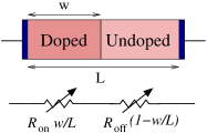
Figure 1: Schematic of a $\mathrm{TiO_{2}}$ memristor of length $L$ made of a doped and an undoped region, and its simplified equivalent circuit. The doped region of length $w$ has resistance $\frac{w}{L}R_{\mbox{\tiny on}}$ and the undoped region has resistance $\left(1-\frac{w}{L}\right)R_{\mbox{\tiny off}}$.

In order to illustrate the above phenomenon in an experimentally realizable system, we consider the model of a memristor presented in Ref. Strukov et al. (2008) (Fig. 1). It consists of a thin film (on the order of a few nanometers) containing one layer of insulating $\mathrm{TiO_{2}}$ and one layer of oxygen-poor $\mathrm{TiO_{2-x}}$ between two metal contacts. Oxygen vacancies in the system act as mobile $+2$ charged dopants. These dopants create a doped $\mathrm{TiO_{2}}$ region whose resistance is much lower than the resistance of the undoped region. The location of the boundary between the doped and undoped regions, and therefore the effective resistance of the film, depends on the position of the dopants and can be modified by applying an external electric field. The mobility of the dopants is ${\mu_{\mbox{\tiny D}}\sim 10^{-10}\,\mathrm{cm^{2}V^{-1}s^{-1}}}$. We take as total size of the memristor $L=10\,\mathrm{nm}$ and denote the length of the doped region as $w$. The current is $I(t)={V(t)}/{M(w)}$ with the effective resistance of the system approximated as Strukov et al. (2008)

$$M(w) = \frac{w}{L}R_{\mbox{\tiny on}}+\left(1-\frac{w}{L}\right)R_{\mbox{\tiny off}}$$ (9)

where $R_{\mbox{\tiny on}}$ is the resistance of the memristor if it is completely doped, and $R_{\mbox{\tiny off}}$ is its resistance if it is undoped. In the following we set $R_{\mbox{\tiny on}}=1\,\mathrm{k\Omega}$ and $R_{\mbox{\tiny off}}=4\,\mathrm{k\Omega}$. The system is controlled by the applied voltage $V(t)=V_{0}\sin\omega_{0}t$. The memristive effect in this model arises from the time dependence of the width of the doped region $w$ Blanc and Staebler (1971)

$$\frac{\mathrm{d}w}{\mathrm{d}t} = \frac{\mu_{\mbox{\tiny D}}R_{\mbox{\tiny on}}}{L}I(t)F\left(\frac{w}{L}\right)+L\xi(t)$$ (10)

where the width is limited by $0<w<L$ and $F(x)=1-(2x-1)^{2}$ suppresses the speed of the boundary between the two regions at the edges $w\sim 0$ and $L$ Joglekar and Wolf (2009). The time scale $t_{0}=\frac{L^{2}}{\mu_{\mbox{\tiny D}}V_{0}}$ is the time required for the dopants to travel a distance $L$ under a constant voltage $V_{0}$.

Let us first assume white Gaussian noise of intensity $\Gamma$

$$\langle\xi(t)\rangle = 0,\ \ \ \ \ \langle\xi(t)\xi(t^{\prime})\rangle=\Gamma\delta(t-t^{\prime}),$$ (11)

which can be tuned experimentally by varying the temperature $T$ of the environment. In fact, using the above definitions the diffusion coefficient is

$$D=\frac{\Gamma L^{2}}{2}$$ (12)

which has to be compared with

$$D=D_{0}\exp\left(-\frac{E_{\nu}}{k_{\mbox{\tiny B}}T}\right)$$ (13)

where $D_{0}\approx 10^{-3}\,\mathrm{cm^{2}/s}$ and $E_{\nu}\approx 0.5\mathrm{eV}$ is the activation energy for oxygen vacancy diffusion Radecka et al. (1999). We note here that the noise in our model was introduced in the simplest possible way such that it shakes the sharp boundary between the doped and undoped regions of the $\mathrm{TiO_{2}}$ memristor. Of course, in the real system the boundary is smeared. However, it was not our intention to present a detailed physical model of the $\mathrm{TiO_{2}}$ memristor, rather to point out an interesting phenomenon due to noise.

Without any noise the size of the hysteresis in the current-voltage characteristic depends on the applied voltage frequency. In particular, at low frequencies ($\omega\ll 2\pi/t_{0}$) the variation of memristance is very small (see Fig. 2) with a consequent small hysteresis loop (Fig. 3).

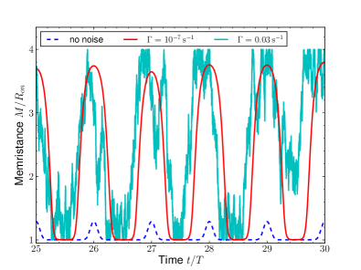
Figure 2: Single realization of the memristance $M(w)$ as a function of time (in units of the time period $T=2\pi/\omega_{0}$) for different noise strengths. The amplitude of the applied voltage is $V_{0}=5.5\,\mathrm{mV}$ and the angular frequency is $\omega=0.25\,\mathrm{Hz}$. The resistance ratio is ${R_{\mbox{\tiny off}}}/{R_{\mbox{\tiny on}}}=4$ and the initial location of the boundary for all simulations is taken as $w_{0}/L=0.9$.

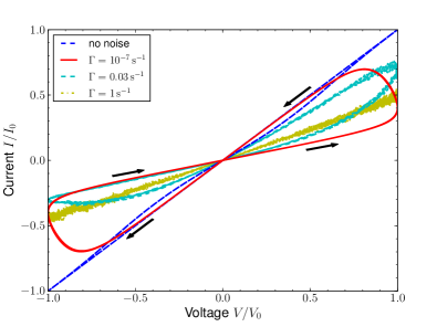
Figure 3: Current-voltage characteristic of the memristor represented in Fig. 1 averaged over $100$ realizations of the stochastic process and for different noise strengths. Here $I_{0}=V_{0}/R_{\mbox{\tiny on}}$ is the maximum possible current through the system. The other parameters are the same as in Fig. 2.

The addition of a small amount of noise does not change this hysteresis loop considerably, but by increasing the noise strength we find an optimal value of $\Gamma$ at which the hysteresis is considerably enhanced. In order to find this value we proceed as follows. For every finite value of the noise strength $\Gamma$ the stochastic differential equation [Eq. (10)] (along with the current and Eq. (9)) is solved (using the Euler-Maruyama method Kloeden and Platen (1992)) and the boundary position $\{w(t)\}_{\xi}$ is calculated for every realization of the stochastic process. The power spectrum (defined as the squared absolute value of the Fourier transform of $\{w(t)\}_{\xi}$) is then computed and averaged over multiple realizations. If the output $\{w(t)\}_{\xi}$ is well synchronized with the external periodic voltage, the power spectrum exhibits a strong peak at the voltage frequency $\omega_{0}$ (Fig. 4). The signal-to-noise ratio (SNR) is then defined as the height of the peak divided by the height of the noise background at frequency $\omega_{0}$. The SNR attains its maximum for the noise strength at which the stochastic resonance occurs (see the inset of Fig. 4). From our simulations we find that the maximum SNR is found for $\Gamma=10^{-7}$s^-1 (Fig. 4) .

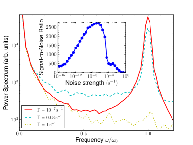
Figure 4: Power spectrum averaged over $100$ realizations. The height of the peak at $\omega=\omega_{0}$ is a measure of synchronization between the applied voltage and the noise. Inset: The signal-to-noise ratio at $\omega=\omega_{0}$ is plotted vs the noise strength and its maximum defines the stochastic resonance.

Fig. 3 indeed confirms that for this value of noise the hysteresis loop is the widest, compared with the loops for other values of noise. In particular, we find that stronger noise destroys the hysteresis loop as intuitively expected.

This picture can be explained qualitatively as follows. When the frequency and amplitude of the external drive are low and the external noise introduced into the system is zero or very weak, the boundary movement closely follows the change in the applied voltage and sweeps a small region of the system . If the noise is very strong, the boundary moves erratically between the edges of the memristor with almost no dependence on the applied voltage. In both cases the hysteresis loop is narrow. Wide loops are obtained whenever the boundary sweeps wide regions following the changes in the voltage. For intermediate values of noise one can expect the noise to ”help” the transitions of the boundary from one edge to the other. Whenever the boundary is moving from, say, the left edge toward the right one, the noise can randomly kick it to the right edge and on the way back kick it back to the left edge providing an almost ideal periodic movement (see Fig. 2).

Finally, we have also checked the effect of introducing colored noise into the system. We have considered noise with an exponentially decaying autocorrelation function

$$\langle\xi(t)\rangle=0,\ \ \langle\xi(t)\xi(t^{\prime})\rangle=\Gamma\exp\left(-\frac{|t-t^{\prime}|}{\tau_{c}}\right)$$ (14)

where $\tau_{c}$ is the correlation time. In this case, we have indeed found (not reported here) enhancement of memory effects even at high frequencies $\omega\gg t_{0}$ with $\tau_{c}\sim t_{0}$. This is not too surprising since, loosely speaking, the addition of this type of noise is reminiscent of the addition of an external driving with frequencies $\omega\lesssim 1/\tau_{c}$.

IV Conclusions

We conclude by noting that the above predictions can be tested experimentally by using memory resistors such as those considered in Ref. Strukov et al. (2008) or any other memory element Pershin and Di Ventra (2011). In a real experiment the frequency and the noise can be easily changed, the latter via, e.g., the external temperature. If we focus again on the model considered here, according to Eq. (13), the diffusion exponentially depends on the temperature. Therefore, if vacancy diffusion is the main mechanism of memory in $\mathrm{TiO_{2}}$ thin films, the opening of the hysteresis should be strongly dependent on the external temperature, at least for small enough frequencies. This can be checked by lowering the frequency of the applied voltage below the optimal one for a wide hysteresis loop, tuning the temperature and observing the change in the shape of the hysteresis. Since the mechanism of memory in this particular memristive system is still under debate, with redox effects at the metal-$\mathrm{TiO_{2}}$ interface the other most probable cause Wu and McCreery (2009); Jeong et al. (2009), the tunability of the noise strength provides a possible diagnostic tool to distinguish between the different mechanisms at play. In general, since in a real system noise is always present, it is highly possible that the hysteresis curves found experimentally in several memory elements Pershin and Di Ventra (2011) could result from the cooperative effect of the optimal frequency in the presence of noise.