J. P. Lees
V. Poireau
V. Tisserand
Laboratoire d’Annecy-le-Vieux de Physique des Particules (LAPP), Université de Savoie, CNRS/IN2P3, F-74941 Annecy-Le-Vieux, France
J. Garra Tico
E. Grauges
Universitat de Barcelona, Facultat de Fisica, Departament ECM, E-08028 Barcelona, Spain
M. MartinelliabD. A. MilanesaA. PalanoabM. PappagalloabINFN Sezione di Baria; Dipartimento di Fisica, Università di Barib, I-70126 Bari, Italy
G. Eigen
B. Stugu
L. Sun
University of Bergen, Institute of Physics, N-5007 Bergen, Norway
D. N. Brown
L. T. Kerth
Yu. G. Kolomensky
G. Lynch
Lawrence Berkeley National Laboratory and University of California, Berkeley, California 94720, USA
H. Koch
T. Schroeder
Ruhr Universität Bochum, Institut für Experimentalphysik 1, D-44780 Bochum, Germany
D. J. Asgeirsson
C. Hearty
T. S. Mattison
J. A. McKenna
University of British Columbia, Vancouver, British Columbia, Canada V6T 1Z1
A. Khan
Brunel University, Uxbridge, Middlesex UB8 3PH, United Kingdom
V. E. Blinov
A. R. Buzykaev
V. P. Druzhinin
V. B. Golubev
E. A. Kravchenko
A. P. Onuchin
S. I. Serednyakov
Yu. I. Skovpen
E. P. Solodov
K. Yu. Todyshev
A. N. Yushkov
Budker Institute of Nuclear Physics, Novosibirsk 630090, Russia
M. Bondioli
S. Curry
D. Kirkby
A. J. Lankford
M. Mandelkern
D. P. Stoker
University of California at Irvine, Irvine, California 92697, USA
H. Atmacan
J. W. Gary
F. Liu
O. Long
G. M. Vitug
University of California at Riverside, Riverside, California 92521, USA
C. Campagnari
T. M. Hong
D. Kovalskyi
J. D. Richman
C. A. West
University of California at Santa Barbara, Santa Barbara, California 93106, USA
A. M. Eisner
J. Kroseberg
W. S. Lockman
A. J. Martinez
T. Schalk
B. A. Schumm
A. Seiden
University of California at Santa Cruz, Institute for Particle Physics, Santa Cruz, California 95064, USA
C. H. Cheng
D. A. Doll
B. Echenard
K. T. Flood
D. G. Hitlin
P. Ongmongkolkul
F. C. Porter
A. Y. Rakitin
California Institute of Technology, Pasadena, California 91125, USA
R. Andreassen
M. S. Dubrovin
B. T. Meadows
M. D. Sokoloff
University of Cincinnati, Cincinnati, Ohio 45221, USA
P. C. Bloom
W. T. Ford
A. Gaz
M. Nagel
U. Nauenberg
J. G. Smith
S. R. Wagner
University of Colorado, Boulder, Colorado 80309, USA
R. Ayad
Now at Temple University, Philadelphia, Pennsylvania 19122, USA
W. H. Toki
Colorado State University, Fort Collins, Colorado 80523, USA
B. Spaan
Technische Universität Dortmund, Fakultät Physik, D-44221 Dortmund, Germany
M. J. Kobel
K. R. Schubert
R. Schwierz
Technische Universität Dresden, Institut für Kern- und Teilchenphysik, D-01062 Dresden, Germany
D. Bernard
M. Verderi
Laboratoire Leprince-Ringuet, Ecole Polytechnique, CNRS/IN2P3, F-91128 Palaiseau, France
P. J. Clark
S. Playfer
J. E. Watson
University of Edinburgh, Edinburgh EH9 3JZ, United Kingdom
D. BettoniaC. BozziaR. CalabreseabG. CibinettoabE. FioravantiabI. GarziaabE. LuppiabM. MuneratoabM. NegriniabL. PiemonteseaINFN Sezione di Ferraraa; Dipartimento di Fisica, Università di Ferrarab, I-44100 Ferrara, Italy
R. Baldini-Ferroli
A. Calcaterra
R. de Sangro
G. Finocchiaro
M. Nicolaci
S. Pacetti
P. Patteri
I. M. Peruzzi
Also with Università di Perugia, Dipartimento di Fisica, Perugia, Italy
M. Piccolo
M. Rama
A. Zallo
INFN Laboratori Nazionali di Frascati, I-00044 Frascati, Italy
R. ContriabE. GuidoabM. Lo VetereabM. R. MongeabS. PassaggioaC. PatrignaniabE. RobuttiaINFN Sezione di Genovaa; Dipartimento di Fisica, Università di Genovab, I-16146 Genova, Italy
B. Bhuyan
V. Prasad
Indian Institute of Technology Guwahati, Guwahati, Assam, 781 039, India
C. L. Lee
M. Morii
Harvard University, Cambridge, Massachusetts 02138, USA
A. J. Edwards
Harvey Mudd College, Claremont, California 91711
A. Adametz
J. Marks
U. Uwer
Universität Heidelberg, Physikalisches Institut, Philosophenweg 12, D-69120 Heidelberg, Germany
F. U. Bernlochner
M. Ebert
H. M. Lacker
T. Lueck
Humboldt-Universität zu Berlin, Institut für Physik, Newtonstr. 15, D-12489 Berlin, Germany
P. D. Dauncey
M. Tibbetts
Imperial College London, London, SW7 2AZ, United Kingdom
P. K. Behera
U. Mallik
University of Iowa, Iowa City, Iowa 52242, USA
C. Chen
J. Cochran
H. B. Crawley
W. T. Meyer
S. Prell
E. I. Rosenberg
A. E. Rubin
Iowa State University, Ames, Iowa 50011-3160, USA
A. V. Gritsan
Z. J. Guo
Johns Hopkins University, Baltimore, Maryland 21218, USA
N. Arnaud
M. Davier
D. Derkach
G. Grosdidier
F. Le Diberder
A. M. Lutz
B. Malaescu
P. Roudeau
M. H. Schune
A. Stocchi
G. Wormser
Laboratoire de l’Accélérateur Linéaire, IN2P3/CNRS et Université Paris-Sud 11, Centre Scientifique d’Orsay, B. P. 34, F-91898 Orsay Cedex, France
D. J. Lange
D. M. Wright
Lawrence Livermore National Laboratory, Livermore, California 94550, USA
I. Bingham
C. A. Chavez
J. P. Coleman
J. R. Fry
E. Gabathuler
D. E. Hutchcroft
D. J. Payne
C. Touramanis
University of Liverpool, Liverpool L69 7ZE, United Kingdom
A. J. Bevan
F. Di Lodovico
R. Sacco
M. Sigamani
Queen Mary, University of London, London, E1 4NS, United Kingdom
G. Cowan
S. Paramesvaran
University of London, Royal Holloway and Bedford New College, Egham, Surrey TW20 0EX, United Kingdom
D. N. Brown
C. L. Davis
University of Louisville, Louisville, Kentucky 40292, USA
A. G. Denig
M. Fritsch
W. Gradl
A. Hafner
E. Prencipe
Johannes Gutenberg-Universität Mainz, Institut für Kernphysik, D-55099 Mainz, Germany
K. E. Alwyn
D. Bailey
R. J. Barlow
G. Jackson
G. D. Lafferty
University of Manchester, Manchester M13 9PL, United Kingdom
R. Cenci
B. Hamilton
A. Jawahery
D. A. Roberts
G. Simi
University of Maryland, College Park, Maryland 20742, USA
C. Dallapiccola
University of Massachusetts, Amherst, Massachusetts 01003, USA
R. Cowan
D. Dujmic
G. Sciolla
Massachusetts Institute of Technology, Laboratory for Nuclear Science, Cambridge, Massachusetts 02139, USA
D. Lindemann
P. M. Patel
S. H. Robertson
M. Schram
McGill University, Montréal, Québec, Canada H3A 2T8
P. BiassoniabA. LazzaroabV. LombardoaF. PalomboabS. StrackaabINFN Sezione di Milanoa; Dipartimento di Fisica, Università di Milanob, I-20133 Milano, Italy
L. Cremaldi
R. Godang
Now at University of South Alabama, Mobile, Alabama 36688, USA
R. Kroeger
P. Sonnek
D. J. Summers
University of Mississippi, University, Mississippi 38677, USA
X. Nguyen
P. Taras
Université de Montréal, Physique des Particules, Montréal, Québec, Canada H3C 3J7
G. De NardoabD. MonorchioabG. OnoratoabC. SciaccaabINFN Sezione di Napolia; Dipartimento di Scienze Fisiche, Università di Napoli Federico IIb, I-80126 Napoli, Italy
G. Raven
H. L. Snoek
NIKHEF, National Institute for Nuclear Physics and High Energy Physics, NL-1009 DB Amsterdam, The Netherlands
C. P. Jessop
K. J. Knoepfel
J. M. LoSecco
W. F. Wang
University of Notre Dame, Notre Dame, Indiana 46556, USA
K. Honscheid
R. Kass
Ohio State University, Columbus, Ohio 43210, USA
J. Brau
R. Frey
N. B. Sinev
D. Strom
E. Torrence
University of Oregon, Eugene, Oregon 97403, USA
E. FeltresiabN. GagliardiabM. MargoniabM. MorandinaM. PosoccoaM. RotondoaF. SimonettoabR. StroiliabINFN Sezione di Padovaa; Dipartimento di Fisica, Università di Padovab, I-35131 Padova, Italy
E. Ben-Haim
M. Bomben
G. R. Bonneaud
H. Briand
G. Calderini
J. Chauveau
O. Hamon
Ph. Leruste
G. Marchiori
J. Ocariz
S. Sitt
Laboratoire de Physique Nucléaire et de Hautes Energies, IN2P3/CNRS, Université Pierre et Marie Curie-Paris6, Université Denis Diderot-Paris7, F-75252 Paris, France
M. BiasiniabE. ManoniabA. RossiabINFN Sezione di Perugiaa; Dipartimento di Fisica, Università di Perugiab, I-06100 Perugia, Italy
C. AngeliniabG. BatignaniabS. BettariniabM. CarpinelliabAlso with Università di Sassari, Sassari, Italy
G. CasarosaabA. CervelliabF. FortiabM. A. GiorgiabA. LusianiacN. NeriabB. OberhofabE. PaoloniabA. PerezaG. RizzoabJ. J. WalshaINFN Sezione di Pisaa; Dipartimento di Fisica, Università di Pisab; Scuola Normale Superiore di Pisac, I-56127 Pisa, Italy
D. Lopes Pegna
C. Lu
J. Olsen
A. J. S. Smith
A. V. Telnov
Princeton University, Princeton, New Jersey 08544, USA
F. AnulliaG. CavotoaR. FacciniabF. FerrarottoaF. FerroniabM. GasperoabL. Li GioiaM. A. MazzoniaG. PireddaaINFN Sezione di Romaa; Dipartimento di Fisica, Università di Roma La Sapienzab, I-00185 Roma, Italy
C. Buenger
T. Hartmann
T. Leddig
H. Schröder
R. Waldi
Universität Rostock, D-18051 Rostock, Germany
T. Adye
E. O. Olaiya
F. F. Wilson
Rutherford Appleton Laboratory, Chilton, Didcot, Oxon, OX11 0QX, United Kingdom
S. Emery
G. Hamel de Monchenault
G. Vasseur
Ch. Yèche
CEA, Irfu, SPP, Centre de Saclay, F-91191 Gif-sur-Yvette, France
D. Aston
D. J. Bard
R. Bartoldus
J. F. Benitez
C. Cartaro
M. R. Convery
J. Dorfan
G. P. Dubois-Felsmann
W. Dunwoodie
R. C. Field
M. Franco Sevilla
B. G. Fulsom
A. M. Gabareen
M. T. Graham
P. Grenier
C. Hast
W. R. Innes
M. H. Kelsey
H. Kim
P. Kim
M. L. Kocian
D. W. G. S. Leith
P. Lewis
S. Li
B. Lindquist
S. Luitz
V. Luth
H. L. Lynch
D. B. MacFarlane
D. R. Muller
H. Neal
S. Nelson
I. Ofte
M. Perl
T. Pulliam
B. N. Ratcliff
A. Roodman
A. A. Salnikov
V. Santoro
R. H. Schindler
A. Snyder
D. Su
M. K. Sullivan
J. Va’vra
A. P. Wagner
M. Weaver
W. J. Wisniewski
M. Wittgen
D. H. Wright
H. W. Wulsin
A. K. Yarritu
C. C. Young
V. Ziegler
SLAC National Accelerator Laboratory, Stanford, California 94309 USA
W. Park
M. V. Purohit
R. M. White
J. R. Wilson
University of South Carolina, Columbia, South Carolina 29208, USA
A. Randle-Conde
S. J. Sekula
Southern Methodist University, Dallas, Texas 75275, USA
M. Bellis
P. R. Burchat
T. S. Miyashita
Stanford University, Stanford, California 94305-4060, USA
M. S. Alam
J. A. Ernst
State University of New York, Albany, New York 12222, USA
R. Gorodeisky
N. Guttman
D. R. Peimer
A. Soffer
Tel Aviv University, School of Physics and Astronomy, Tel Aviv, 69978, Israel
P. Lund
S. M. Spanier
University of Tennessee, Knoxville, Tennessee 37996, USA
R. Eckmann
J. L. Ritchie
A. M. Ruland
C. J. Schilling
R. F. Schwitters
B. C. Wray
University of Texas at Austin, Austin, Texas 78712, USA
J. M. Izen
X. C. Lou
University of Texas at Dallas, Richardson, Texas 75083, USA
F. BianchiabD. GambaabINFN Sezione di Torinoa; Dipartimento di Fisica Sperimentale, Università di Torinob, I-10125 Torino, Italy
L. LanceriabL. VitaleabINFN Sezione di Triestea; Dipartimento di Fisica, Università di Triesteb, I-34127 Trieste, Italy
N. Lopez-March
F. Martinez-Vidal
A. Oyanguren
IFIC, Universitat de Valencia-CSIC, E-46071 Valencia, Spain
H. Ahmed
J. Albert
Sw. Banerjee
H. H. F. Choi
G. J. King
R. Kowalewski
M. J. Lewczuk
C. Lindsay
I. M. Nugent
J. M. Roney
R. J. Sobie
University of Victoria, Victoria, British Columbia, Canada V8W 3P6
T. J. Gershon
P. F. Harrison
T. E. Latham
E. M. T. Puccio
Department of Physics, University of Warwick, Coventry CV4 7AL, United Kingdom
H. R. Band
S. Dasu
Y. Pan
R. Prepost
C. O. Vuosalo
S. L. Wu
University of Wisconsin, Madison, Wisconsin 53706, USA
Abstract
We present a study of
the decays with mesons
reconstructed in the or final states,
where indicates a or a meson.
Using a sample of million pairs collected with
the BABAR detector at the PEP-II asymmetric-energy collider
at SLAC, we measure the ratios . We obtain and
, from which we extract the upper limits
at 90% probability: and . Using these measurements, we
obtain an upper limit for the ratio of the magnitudes of the and
amplitudes at 90% probability.
pacs:
13.25.Hw, 14.40.Nd
I Introduction
violation effects are described in the Standard Model (SM) of
elementary particles with a single phase in the
Cabibbo-Kobayashi-Maskawa (CKM) quark mixing matrix
cite:ckm . One of the unitarity
conditions for this matrix can be interpreted as
a triangle in the plane of Wolfenstein parameters cite:Wolf ,
where one of the angles is
. Various
methods to determine using decays
have been proposed cite:GLW ; cite:ADS ; cite:DKDalitz .
In this paper, we consider the decay channel with cite:charge studied through the
Atwood-Dunietz-Soni (ADS) method cite:ADS . In this method the final
state under consideration can be reached through and
processes as indicated in Fig. 1 that are followed by either
Cabibbo-favored or Cabibbo suppressed decays. The interplay between different
decay channels leads to a possibility to extract the angle alongside with other parameters
for these decays.
Figure 1: Feynman diagrams for (top, transition) and
(bottom, transition).
Following the ADS method, we search for events, where the
favored decay, followed by the doubly-
Cabibbo-suppressed decay, interferes with the
suppressed decay, followed by the
Cabibbo-favored decay. These are called
“opposite-sign” events because the two kaons in the final state
have opposite charges. We also reconstruct a larger sample of
“same-sign” events, which mainly arise from the favored decays followed by the Cabibbo-favored decays. We define and . We extract
(1)
(2)
from the selected and samples, respectively.
While our previous analysis cite:ViolaADS used another set of observables:
(3)
(4)
we prefer to use observables defined in Eqs. 1 and 2 since their
statistical uncertainties, which dominate in the final error
of this measurement, are uncorrelated.
The amplitude of the two-body decay can be written as
(5)
where is the ratio of the magnitudes of the and amplitudes,
is the conserving strong phase, and is the violating weak phase.
For the three-body decay we use similarly defined variables:
(6)
(7)
where and are the magnitude of the
Cabibbo-favored and doubly-Cabibbo-Suppressed amplitudes, respectively,
is the relative strong phase, and indicates a position in the Dalitz plot of
squared invariant masses . The parameter , called the coherence factor, can
take values in the interval .
Neglecting -mixing effects, which in the SM
give negligible corrections to and do not affect the
measurement, the ratios and are related to
the - and -mesons’ decay parameters through the following relations:
(8)
(9)
with . The values
of and measured by the CLEO-c
collaboration cite:CLEO , and
, are used in the
signal yield estimation and
extraction. The ratio has been
measured in different experiments and we take the average value
cite:PDG . Its value
is small compared to the present determination of
, which is taken to be cite:UTFIT .
According to Eqs. 8 and 9, this implies that the
measurements of ratios is mainly sensitive to
. For the same reason, the
sensitivity to is reduced, and
therefore the main aim of this analysis is to measure , , and .
The current high precision on is based on several earlier analyses
by the BABARcite:ViolaADS ; cite:BaBarADS ; cite:BaBarDalitz ; cite:BaBarGLW ,
BELLE cite:BelleADS ; cite:BelleDalitz ; cite:BelleGLW , and CDF cite:CDFGLW collaborations.
This paper is an update of our previous analysis cite:ViolaADS based on
pairs and resulting in a measurement of ,
which was translated into
the confidence level limit .
The results
presented in this paper are obtained with 431 of
data collected at the resonance with the BABAR detector
at the PEP-II collider at SLAC, corresponding to
pairs. An additional “off-resonance” data sample of
45 , collected at a center-of-mass (CM) energy 40 below the
resonance, is used to study backgrounds from “continuum”
events, ( or ).
II Event Reconstruction and Selection
The BABAR detector is described in detail
elsewhere cite:det . Charged-particle tracking is performed by
a five-layer silicon vertex tracker (SVT) and a 40-layer drift
chamber (DCH). In addition to providing precise position information
for tracking, the SVT and DCH measure the specific ionization, which
is used for identification of low-momentum charged
particles. At higher momenta pions and kaons are
distinguished by Cherenkov radiation detected in a ring-imaging device
(DIRC). The positions and energies of photons are measured with an
electromagnetic calorimeter (EMC) consisting of 6580 thallium-doped
CsI crystals. These systems are mounted inside a 1.5 T solenoidal
superconducting magnet. Muons are identified by the instrumented
flux return, which is located outside the magnet.
The event selection is based on studies of off-resonance data
and Monte Carlo (MC) simulations of continuum and events. The BABAR detector response
is modeled with Geant4cite:geant4 .
We also use EvtGencite:EVTGEN to model
the kinematics of meson decays and JetSetcite:jetset
to model continuum background processes. All selection criteria are
optimized by maximizing the ratio,
where and are the expected numbers of
the opposite-sign signal and background events, respectively.
In the optimization we assume an opposite-sign branching fraction
of cite:PDG .
The charged kaon and pion identification criteria are based on a likelihood technique.
These criteria are typically 85% efficient, depending on the momentum and
polar angle, with misidentification rates at the 2% level.
The candidates are reconstructed from pairs of photon
candidates with an invariant mass in the interval
and with total energy
greater than 200. Each photon should have energy greater than 70 .
The neutral meson candidates are reconstructed from a charged
kaon, a charged pion, and a neutral pion. The correlation between
the tails in the distribution of the invariant mass,
, and the candidate mass, , is taken into
account by requiring to be within
of its nominal value cite:PDG , which is times the experimental resolution.
The candidates are reconstructed by combining and candidates, and constraining them to originate from a common vertex. The
probability distribution of the cosine of the polar angle with
respect to the beam axis in the CM frame, , is
expected to be proportional to . We require
.
We measure two almost independent kinematic variables: the
beam-energy substituted mass
,
and the energy difference , where
and are the energy and momentum, the subscripts and
refer to the candidate meson and system,
respectively, is the center-of-mass energy, and
is measured in the CM frame. For correctly reconstructed mesons the distribution of
peaks at the mass, and the distribution of peaks at zero. The candidates are
required to have in the range ( standard deviations).
We consider only events with in the range
.
In less than 2% of the events, multiple candidates are present, and in these cases we choose
that with a
reconstructed mass closest to the nominal mass
value cite:PDG . If more than one candidate share the
same candidate, we select that
with the smallest . In the following we refer to the selected
candidate as .
All charged and neutral reconstructed particles not associated with
, but with the other decay in the event, , are called the rest of the event.
III Background Characterization
After applying the selection criteria described above, the remaining
background is composed of non-signal events and continuum
events. Continuum background events, in contrast to events, are
characterized by a jet-like topology. This difference
can be exploited to discriminate between
the two categories of events by means of a Fisher
discriminant ,
which is a linear combination of six
variables. The coefficients of the linear combination are
chosen to maximize the separation between
signal and continuum background so
that peaks at for signal and at for
continuum background. They are determined with samples of
simulated signal and continuum events, and validated using
off-resonance data.
In the Fisher discriminant we use the absolute value of the cosine of
the angle between and
thrust axes,
where the thrust axis is defined as the direction
maximizing the sum of the longitudinal momenta of all the
particles. Other variables included in are the event shape
moments , and , where the index runs over all tracks and energy
deposits in the rest of the event; is the momentum; and
is the angle with respect to the thrust axis of the .
These three variables are calculated in the CM system. We also
use the distance between the decay vertices
of and , the distance of closest approach
between meson tracks belonging to signal decay chain, and , the absolute value of the
proper time interval between the and
decays Aubert:2002rg . The latter
is calculated using the measured separation
along the beam direction between the decay points of
and and the Lorentz boost of
the CM frame. The decay point is obtained from
tracks that do not belong to the reconstructed , with constraints
from the momentum and the beam-spot location.
We use and to define two regions: the fit region,
defined as and , and the
signal region, defined as and .
The background is divided into two components: non-peaking
(combinatorial) and peaking. The latter consists of -meson
decays that have a well-pronounced peak in the signal region.
One of the decay channels which can mimic opposite-sign signal
events, is the decay with and
. In order to reduce this contribution, we
veto events for which the invariant pair mass is
(with the meson invariant mass, ,
taken to be cite:PDG ). Simulations indicate that the
remaining background is negligible.
Another possible source of peaking background is the decay
with , which can
contribute to the signal region of the same-sign sample due to the
misidentification of the as a . The number of events is expected
to be about 8% of the total same-sign signal sample (see
Table 1).
The charmless decay can also
contribute to the signal region.
The branching fraction of this decay has not been measured. Therefore
the size of this background is estimated from the sidebands of the reconstructed mass,
or
. The result of the study is reported in
Table 1. In the final fit, we fix the yield of
the same-sign peaking background to the sum of charmless and
open-charm events. The opposite-sign background in the final event sample is assumed to be negligible.
The overall reconstruction efficiency for signal events is for opposite-sign signal events and for
same-sign signal events. These numbers are equal within the uncertainty as expected.
The composition of the final
sample is shown in Table 1.
Table 1: Composition of the final selected
sample as evaluated from the MC samples normalized to data and from data
for the
charmless peaking background. The signal contribution is estimated
using values of branching fractions from the PDG cite:PDG and
cite:UTFIT . The errors are from the statistics of the control samples only.
Sample
Region
Signal
non-peaking
Continuum
Charmless peaking
Same sign
Fit
Signal
Opposite sign
Fit
-
Signal
-
IV Fit Procedure and Results
To measure the ratios and we perform extended maximum-likelihood fits to the and distributions, separately for the and data samples. We write
the extended likelihood functions as:
where , , and are the probability density functions (PDFs) of
the hypotheses that the event is a same-sign signal, opposite-sign signal, or a
background event ( are the different background categories
used in the fit), respectively, is the number of events in the
selected sample, and is the expectation value for the total number
of events. The symbol
indicates the set of parameters to be fitted.
is the total number of signal events,
for the decays of
the meson, and is the total number of events of each background
component. For the opposite-sign events the background comes
from continuum and events. The peaking background
is introduced as a separate component in the fit to the same-sign sample. The fit is performed to the
sample (consisting of 15706 events) to determine and to the sample (consisting of 15057 events) to determine
. The PDFs for and fits are identical.
The ratio is fitted to the same likelihood ansatz, but to the combined and data sample.
Since the correlations among the
variables are negligible, we write the PDFs as products of the
one-dimensional distributions of and . The absence of
correlation between these distributions is checked using MC
samples. The signal distributions is modeled with the same
asymmetric Gaussian function for both same-sign and opposite-sign
events, while the distribution is taken as a sum of two
Gaussians. The continuum background distributions for the same and
opposite-sign events are modeled
with two different threshold ARGUS functions cite:argus
defined as follows:
(10)
where represents the maximum allowed value for the variable
, and determines the shape of the distribution. The distribution of the non-peaking background components are modeled
with Crystal Ball (CB) functions that are different for same-sign and
opposite-sign events cite:CB . The CB function is a Gaussian
modified to include a power-law tail on the low side of the peak.
The distributions for the background are approximated with
sums of two asymmetric Gaussians. For the peaking background we
conservatively use the same parameter set as for the signal.
The PDF parameters are derived from data when possible. The
parameters for continuum events are determined from the
off-resonance data sample. The parameters for the distribution
of signal events are extracted from the sample of
with , while for the parameters of the
signal Fisher PDF we use the MC sample. The parameters of non-peaking
distributions are
determined from the MC sample.
From each fit, we extract the ratios , , or , the total number of
signal events in the sample () along with the non-peaking background yields and threshold function slope
for the continuum background. We fix the number of peaking background events.
To test the fitting procedure we generated 10000 pseudo-experiments based on the PDFs described above.
The fitting procedure is then tested on
these samples. We find no bias in the number of fitted events for
any component of the fit. Tests of the fit procedure performed on
the full MC samples give values for the yields compatible with those expected.
Table 2: Results of fits to the , , and the combined and samples, including
the extracted number of signal and background events and their statistical errors.
Sample
and
The main results of the fit to the data
are summarized in Table 2.
The fits to the for and the distribution with
are shown in Fig. 2, for the combined and sample.
These restrictions reduce the background and retain most of the signal events.
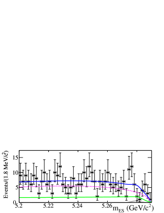
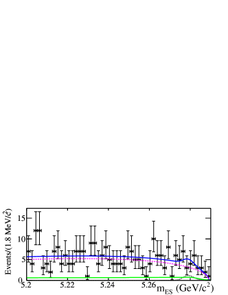
Fig. 3 shows the fits for the separate and samples.
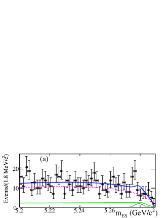
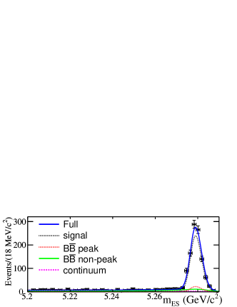
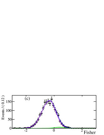
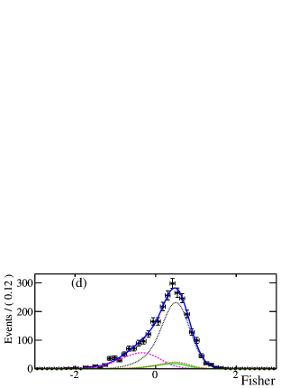
Figure 2: (color online) Distribution of (a,b) (with ) and (c,d) (with )
and the results of the maximum likelihood fits for the combined and samples (extracting ),
for (a,c) opposite-sign and (b,d) same-sign decays. The data are well described by the overall fit result (solid blue line)
which is the sum of the signal, continuum, non-peaking, and peaking backgrounds.
Figure 3: (color online) Projections of the 2D likelihood for with
the additional requirement
, obtained from the fit to the (left) and
(right) data sample for opposite-sign events (extracting and ).
The labeling of the curves is the same as in Fig. 2.
V Systematic Uncertainties
We consider various sources of systematic uncertainties, listed in Table 3.
One of the largest
contributions comes from the uncertainties on the PDF
parameters. To evaluate the contributions related to the
and PDFs, we repeat the fit varying the
PDF parameters for each fit species within their statistical errors, taking
into account correlations among the parameters (labeled as “PDF
error” in Table 3).
To evaluate the uncertainties arising from peaking background
contributions, we repeat the fit varying the the peaking background contribution within its statistical uncertainties
and the errors of branching
fractions, , used
to estimate the contribution. For the
opposite-sign events only the positive part of the probability distribution
is used in the evaluation.
Differences between data and MC (labeled as “Simulation” in Table 3) in
the shape of the distribution are studied for signal components
using the data control samples of with
. These parameters are expected to be slightly different
between the and samples.
We conservatively take the systematic uncertainty
as the difference in the fit results from the nominal
parameters set (using MC events) and the parameters set obtained using
the data sample.
The systematic uncertainty attributed to the crossfeed between
opposite-sign and same-sign events has been evaluated from the MC
samples. The number of same-sign events passing the selection of the
opposite-sign events is taken as a systematic uncertainty.
The efficiencies for same-sign and
opposite-sign events were verified to be the same within a precision of
3% cite:ViolaB0 . We
hence assign a systematic uncertainty on based on variations due to changes in the efficiency ratio by .
The systematic uncertainties for the ratios , , and are summarized in Table 3.
The overall systematic errors represent the sum in quadrature of the individual uncertainties.
Table 3: Systematic errors for
and in units of .
Source
PDF error
1.1
1.0
Same sign peaking background
0.2
0.5
0.2
Opposite sign peaking background
Simulation
0.6
0.6
0.7
errors
0.2
0.6
0.4
Crossfeed contribution
0.1
0.4
0.3
Efficiency ratio
0.1
0.4
0.3
Combined uncertainty
VI Extraction of
Following a Bayesian approach cite:bayes , the probability distributions for the
and ratios obtained in the fit
are translated into a probability distribution for using
Eqs. 8 and 9 simultaneously. We assume the following prior
probability distributions: for a Gaussian with mean
and standard deviation cite:PDG ;
for and , we use the likelihood obtained in Ref. cite:CLEO ,
taking into account a 180 degree difference in the phase convention for ;
for and we assume a uniform distribution
between 0 and 360 degrees, while for a uniform
distribution in the range is used.
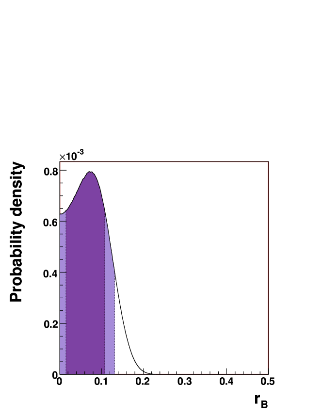
We obtain the posterior probability distribution shown in Fig. 4.
Since the measurements are not statistically significant, we
integrate over the positive portion of that distribution
and obtain the upper limit
at 90% probability,
and the range
(11)
and 0.078 as the most probable value.
Figure 4: Bayesian posterior probability density
function for from our measurement of
and and the hadronic decay
parameters , , and taken
from cite:CLEO and cite:PDG .
The dark and light shaded zones represent the
68% and 90% probability regions, respectively.
VII Summary
We have presented a study of the decays and , in which the and mesons
decay to the final state
using the ADS method. The analysis is performed using
pairs, the full BABAR dataset. Previous
results cite:ViolaADS are improved and superseded
by improved event reconstruction algorithms and analysis strategies
employed on a larger data sample.
The final results are:
(12)
(13)
(14)
from which we obtain 90% probability limits:
(15)
(16)
(17)
From our measurements we derive the limit
(18)
VIII Acknowledgments
We are grateful for the
extraordinary contributions of our PEP-II colleagues in
achieving the excellent luminosity and machine conditions
that have made this work possible.
The success of this project also relies critically on the
expertise and dedication of the computing organizations that
support BABAR.
The collaborating institutions wish to thank
SLAC for its support and the kind hospitality extended to them.
This work is supported by the
US Department of Energy
and National Science Foundation, the
Natural Sciences and Engineering Research Council (Canada),
the Commissariat à l’Energie Atomique and
Institut National de Physique Nucléaire et de Physique des Particules
(France), the
Bundesministerium für Bildung und Forschung and
Deutsche Forschungsgemeinschaft
(Germany), the
Istituto Nazionale di Fisica Nucleare (Italy),
the Foundation for Fundamental Research on Matter (The Netherlands),
the Research Council of Norway, the
Ministry of Education and Science of the Russian Federation,
Ministerio de Ciencia e Innovación (Spain), and the
Science and Technology Facilities Council (United Kingdom).
Individuals have received support from
the Marie-Curie IEF program (European Union), the A. P. Sloan Foundation (USA)
and the Binational Science Foundation (USA-Israel).
References
(1) N. Cabibbo, Phys. Rev. Lett. 10 531 (1963);
M. Kobayashi and T. Maskawa, Prog. Theor. Phys. 49 652 (1973).
(2) L. Wolfenstein, Phys. Rev. Lett. 51, 1945 (1983).
(3) M. Gronau and D. London, Phys. Lett. B253, 483 (1991);
M. Gronau and D. Wyler, Phys. Lett. B265, 172 (1991).
(4) I. Dunietz, Phys. Lett. B270, 75 (1991);
I. Dunietz, Z. Phys. C56, 129 (1992);
D. Atwood, G. Eilam, M. Gronau, and A. Soni, Phys. Lett. B341, 372 (1995);
D. Atwood, I. Dunietz and A. Soni, Phys. Rev. Lett. 78, 3257 (1997).
(5) A. Giri, Yu. Grossman, A. Soffer, and J. Zupan, Phys. Rev. D68, 054018 (2003).
(6) Charge conjugate processes are assumed throughout the paper.
(7) B. Aubert et al. (BABAR Collaboration), Phys. Rev. D76, 111101 (2007).
(8) N. Lowrey et al. (CLEO Collaboration), Phys. Rev. D 80, 031105(R) (2009).
(9) K. Nakamura et al. (Particle Data Group), J. Phys. G 37, 075021 (2010).
(10) M. Bona et al. (UTfit Collaboration), JHEP 0507, 028 (2005). Updated results available at http://www.utfit.org/.
(11) P. del Amo Sanchez et al. (BABAR Collaboration), Phys. Rev. D 82, 072004 (2010).
(12) P. del Amo Sanchez et al. (BABAR Collaboration), Phys. Rev. D 82, 072006 (2010).
(13) P. del Amo Sanchez et al. (BABAR Collaboration), Phys. Rev. Lett. 105, 121801 (2010).
(14) K. Abe et al. (Belle Collaboration), Phys. Rev. D 73 051106 (2006).
(15) Y. Horii et al. (Belle Collaboration), [arXiv:1103.5951].
(16) A. Poluektov et al. (Belle Collaboration), Phys. Rev. D 81, 112002 (2010).
(17) T. Aaltonen et al. (CDF Collaboration), Phys. Rev. D 81, 031105 (2010).
(18) B. Aubert et al. (BABAR Collaboration), Nucl. Instr. Methods A479, 1 (2002).
(19) S. Agostinelli et al. (GEANT4 Collaboration), Nucl. Instrum. Meth. A 506, 250 (2003).
(20) D. J. Lange, Nucl. Instrum. Meth. A 462, 152 (2001).
(21) T. Sjostrand, Comput. Phys. Commun. 82, 74 (1994).
(22) B. Aubert et al. (BABAR Collaboration), Phys. Rev. D 66, 032003
(2002).
(23) H. Albrecht et al. (ARGUS Collaboration), Z. Phys. C48, 543 (1990).
(24) M. J. Oreglia, Ph.D. Thesis, SLAC-236(1980), Appendix D; J. E. Gaiser, Ph.D Thesis, SLAC-255(1982), Appendix F; T. Skwarnicki, Ph.D Thesis, DESY F31-86-02(1986), Appendix E.
(25) B. Aubert et al. (BABAR Collaboration], Phys. Rev. D 80, 031102 (2009).
(26) G. D’Agostini, CERN Report ; G. D’Agostini and M. Raso, arXiv:hep-ex/0002056.