Randomness and differentiability (long version)

Abstract.

We characterize some major algorithmic randomness notions via differentiability of effective functions.

(1) As the main result we show that a real number $z\in[0,1]$ is computably random if and only if each nondecreasing computable function $[0,1]\rightarrow\mathbb{R}$ is differentiable at $z$.

(2) We prove that a real number $z\in[0,1]$ is weakly 2-random if and only if each almost everywhere differentiable computable function $[0,1]\rightarrow\mathbb{R}$ is differentiable at $z$.

(3) Recasting in classical language results dating from 1975 of the constructivist Demuth, we show that a real $z$ is Martin-Löf random if and only if every computable function of bounded variation is differentiable at $z$, and similarly for absolutely continuous functions.

We also use our analytic methods to show that computable randomness of a real is base invariant, and to derive other preservation results for randomness notions.

1. Introduction

The main thesis of this paper is that algorithmic randomness of a real is equivalent to differentiability of effective functions at the real. In more detail, for every major algorithmic randomness notion, one can provide a class of effective functions on the unit interval so that

($*$)   a real $z\in[0,1]$ satisfies the randomness notion $\ \Leftrightarrow\$

each function in the class is differentiable at $z$.

For instance, $z$ is computably random $\ \Leftrightarrow\$ each computable nondecreasing function is differentiable at $z$. Furthermore, $z$ is Martin-Löf random $\ \Leftrightarrow\$ each computable function of bounded variation is differentiable at $z$. The second result was proved by Demuth [7], who used constructive language; we will reprove it here in the usual language, using the first result relativized to an oracle set.

Classically, to say that a property holds for a “random” real $z\in[0,1]$ simply means that the reals failing the property form a null set. For instance, a well-known theorem of Lebesgue [17] states that every nondecreasing function $f\colon\,[0,1]\to{\mathbb{R}}$ is differentiable at all reals $z$ outside a null set (depending on $f$). That is, $f^{\prime}(z)$ exists for a random real $z$ in the sense specified above. Via Jordan’s result that each function of bounded variation is the difference of two nondecreasing functions (see, for instance, [2, Cor 5.2.3]), Lebesgue’s theorem can be extended to functions of bounded variation.

In most of the results of the type ($*$) above, the implication “$\ \Rightarrow\$” can be seen as an effective form of Lebesgue’s theorem. Before we make this precise, we will provide some background on algorithmic randomness, and computable functions on the unit interval.

1.1. Some background

Algorithmic randomness. The idea in algorithmic randomness is to think of a real as random if it is in no effective null set. To specify an algorithmic randomness notion, one has to specify a type of effective null set, which is usually done by introducing a test concept. Failing the test is the same as being in the null set.

A hierarchy of algorithmic randomness notions has been developed, each one corresponding to certain aspects of our intuition. Traditionally, the central notion has been Martin-Löf randomness. A $\Sigma^{0}_{1}$ set $\mathcal{G}\subseteq[0,1]$ has the form $\bigcup_{m}A_{m}$, where $A_{m}$ is an open interval with dyadic rational endpoints obtained effectively from $m$. Let $\mathbf{\lambda}$ denote the usual Lebesgue measure on the unit interval. A Martin-Löf test is a sequence of uniformly $\Sigma^{0}_{1}$ sets $(\mathcal{G}_{m})_{m\in{\mathbb{N}}}$ in the unit interval such that $\mathbf{\lambda}\mathcal{G}_{m}\leq 2^{-m}$ for each $m$. The algorithmic null set it describes is $\bigcap_{m}\mathcal{G}_{m}$.

Schnorr [27] maintained that Martin-Löf randomness is already too powerful to be considered algorithmic, because it is based on computably enumerable objects as tests. He proposed a weaker notion: a real is called computably random if no computable betting strategy can win on its binary expansion (see Subsection 3.1 for detail). We will see that this is the appropriate notion for studying almost-everywhere differentiability of important classes of computable functions.

A $\Pi^{0}_{2}$ set (or effective $G_{\delta}$ set) is of the form $\bigcap_{m}\mathcal{G}_{m}$, where $(\mathcal{G}_{m})_{m\in{\mathbb{N}}}$ is a sequence of uniformly $\Sigma^{0}_{1}$ sets. We call a real weakly $2$-random if it is in no null $\Pi^{0}_{2}$ set. Compared to Martin-Löf randomness, the test notion is relaxed by replacing the condition $\forall m\,\mathbf{\lambda}\mathcal{G}_{m}\leq 2^{-m}$ above by the weaker condition $\lim_{m}\mathbf{\lambda}\mathcal{G}_{m}=0$. For background on algorithmic randomness see [20, Chapter 3] or [21].

Computable functions on the unit interval. Several definitions of computability for a function $f\colon[0,1]\rightarrow\mathbb{R}$ have been proposed. In close analogy to the Church-Turing thesis, many (if not all) of them turned out to be equivalent. The common notion comes close to being a generally accepted formalization of computability for functions on the unit interval. Functions that are intuitively computable, such as $e^{x}$ and $\sqrt{x}$, are computable in this formal sense. Computable functions in that sense are necessarily continuous; see the discussion in Weihrauch [28]. The generally accepted notion goes back to work of Grzegorczyk and Lacombe from the 1950s, as discussed in Pour-El and Richards prior to [23, Def.  A, p. 25]. In the same book [23, Def.  C, p. 26] they give a simple condition equivalent to computability of $f$, which they call “effective Weierstrass”:

$f\colon[0,1]\rightarrow\mathbb{R}$ is computable $\Leftrightarrow$ there is an effective sequence $(P_{n})_{n\in{\mathbb{N}}}$ of polynomials with rational coefficients such that $||f-P_{n}||_{\infty}\leq 2^{-n}$ for each $n$.

This can be interpreted as saying that $f$ is a computable point in a suitable computable metric space. See Subsection 2.2 for another characterization.

1.2. Results of type ($*$): the implication “$\Rightarrow$”

(a) We will show in Theorem 4.1 that

a real $z\in[0,1]$ is computably random $\Rightarrow$

each nondecreasing computable function is differentiable at $z$.

This is an effectivization of Lebesgue’s theorem in terms of the concepts given above. Lebesgue’s theorem is usually proved via Vitali coverings. This method is non-constructive; a new approach is needed for the effective version. The proof is by contraposition. The main problem is to proceed from the non-existence of $f^{\prime}(z)$, which is based on the behaviour of slopes at arbitrarily small intervals $I$ containing $z$, to the success of a betting strategy, which only has access to basic dyadic intervals (namely, intervals of the form $[i2^{-n},(i+1)2^{-n})$ for $n\in{\mathbb{N}},i<2^{n}$). The solution is to bet with scaled and shifted basic dyadic intervals, and show that the scaling and shifting parameters taken from a finite set are sufficient to approximate $I$ from the outside and also from the inside by such intervals.

(b) The corresponding result of Demuth [7] involving Martin-Löf randomness and computable functions of bounded variation will be re-obtained as a corollary, using an effective form of Jordan’s theorem. We note that Demuth’s proof is somewhat obscure, which is partly due to the fact that it is uses constructive language and notation. The attribution to Demuth relies on an interpretation, rather than a straightforward reading, of [7].

(c) For weak $2$-randomness, we take the largest class of computable functions that makes sense in this setting: the almost everywhere differentiable computable functions. The implication $\Rightarrow$ is obtained by observing that the points of nondifferentiablity for any computable function is a $\Sigma^{0}_{3}$ set (i.e., an effective $G_{\delta\sigma}$ set). If the function is a.e. differentiable, this set is null, and hence cannot contain a weakly $2$-random real.

1.3. Results of type ($*$): the implication “$\Leftarrow$”

This is typically proved by contraposition. One simulates tests by non-differentiability of functions. Thus, given a test in the sense of the algorithmic randomness notion, one builds a computable function $f$ on the unit interval such that, for each real $z$ failing the test, $f^{\prime}(z)$ fails to exist. We will provide direct, uniform constructions of this kind for weak $2$-randomness (c), and then for Martin-Löf randomness (b). The computable functions we build are sums of “sawtooth functions”. For computable randomness (a), the simulation is less direct, though still uniform. The results in more detail are as follows.

(a) For each real $z$ that is not computably random, there is a computable nondecreasing function $f$ such that $\overline{D}f(z)=\infty$ (Theorem 4.1).

(b) There is, in fact, a single computable function $f$ of bounded variation such that $f^{\prime}(z)$ fails to exist for all non-Martin-Löf random reals $z$ (Lemma 6.5).

(c) For each $\Pi^{0}_{2}$ null set there is an a.e. differentiable computable function $f$ that is non-differentiable at any $z$ in the null set (Theorem 6.1).

As mentioned above, (b) was already stated by Demuth [7, Example 2]. For background on Demuth’s work see the survey [16].

The implication “$\Leftarrow$” is also rooted in results from classical analysis. For instance, Zahorski [29] proved that each null $G_{\delta}$ subset of ${\mathbb{R}}$ is the non-differentiability set of a monotonic Lipschitz function. For a recent proof, see Fowler and Preiss [13].

1.4. Classes of effective functions, and randomness notions

The results of type ($*$) mean that all the major algorithmic randomness notions for a real can now be matched with at least one class of effective functions on the unit interval in such a way that randomness of a real is equivalent to differentiability at the real. The analytical properties of functions we use are the well-known ones from classical real analysis.

The matching is onto, but not 1-1: in a sense, randomness notions are coarser than classes of effective functions. Computable randomness is characterized not only by differentiability of nondecreasing computable functions, but also of computable Lipschitz functions [14]. Furthermore, as an effectiveness condition on functions, one can choose anything between computability in the sense discussed in Subsection 1.1 above, and the weaker condition that $f(q)$ is a computable real (see Subsection 2.1), uniformly in a rational $q\in[0,1]$. Several notions lying in between have received attention. One of them is Markov computability, which will be discussed briefly in Section 7. Note that for nondecreasing continuous functions, the effectivity notions coincide by Proposition 2.2.

A further well-studied algorithmic randomness notion is Schnorr randomness, which is even weaker than computable randomness (see, for instance, [20, Section 3.5]). A Schnorr test is a Martin-Löf test $(\mathcal{G}_{m})_{m\in{\mathbb{N}}}$ such that $\mathbf{\lambda}\mathcal{G}_{m}$ is a computable real uniformly in $m$. A real $z$ is Schnorr random if $z\not\in\bigcap_{m}\mathcal{G}_{m}$ for each Schnorr test $(\mathcal{G}_{m})_{m\in{\mathbb{N}}}$.

To characterize Schnorr randomness in terms of differentiability, we need a stronger notion of effectivity for functions. Call a function $f$ variation computable if it is a computable point in the Banach space $AC_{0}[0,1]$ of absolutely continuous functions vanishing at $0$, where the norm of a function is its variation on $[0,1]$. The computable structure (in the sense of [23, Ch. 2]) is given, for instance, by the polynomials with rational coefficients. Thus, $f\in AC_{0}[0,1]$ is variation computable iff for each $n$, one can determine a polynomial $P_{n}$ with rational coefficients, vanishing at $0$, such that the variation of $f-P_{n}$ is at most $2^{-n}$. By the effective version of a classical theorem from analysis (see, for instance, [5, Ch. 20]), $AC_{0}[0,1]$ is effectively isometric with the space $(\mathcal{L}_{1}[0,1],||.||_{1})$, where the computable structure is also determined by the polynomials with rational coefficients. The isometry is given by differentiation, and its inverse by the indefinite integral.

Recent results of J. Rute [26], and independently Pathak, Rojas and Simpson, can be restated as follows: $z$ is Schnorr random $\Leftrightarrow$ each absolutely continuous function that is computable in the variation norm is differentiable at $z$. Freer, Kjos-Hanssen, and Nies [14] showed the analogous result for Lipschitz functions.

The matching between algorithmic randomness notions and classes of effective functions is summarized in Figure 1.

Figure 1. Randomness notions matched with classes of effective functions defined on $[0,1]$ so that ($*$) holds

1.5. Discussion

The results above indicate a rich two-way interaction between algorithmic randomness and analysis.

Analysis to randomness: Characterizations via differentiability can be used to improve our understanding of an algorithmic randomness notion. For instance, we will show that several randomness notions of reals are preserved under the maps $z\to z^{\alpha}$ where $\alpha\neq 0$ is a computable real. Furthermore, we show that computable randomness of a real is base invariant: it does not depend on the fact that one uses the binary expansion of a real in its definition (Theorem 3.7 below).

Randomness to analysis: the results also improve our understanding of the underlying classical theorems. They indicate that in the setting of Lebesgue’s theorem mentioned close to the beginning of the paper, the exception sets for differentiability of nondecreasing functions are simpler than the exception sets for functions of bounded variation. Furthermore, one can attempt to calibrate, in the sense of reverse mathematics, the strength of theorems saying that a certain function is a.e. well behaved. The benchmark principles have the form “for each oracle set $X$, there is a set $R$ that is random in $X$”, for some fixed algorithmic randomness notion. For Martin-Löf randomness, the principle above is called “weak weak König’s Lemma”. Now consider the principle that every function of bounded variation is differentiable at some real. By the work in Subsection 7.2 below, this implies weak weak König’s Lemma over a standard base theory called RCA₀. Recent work of Nies and Yokoyama (see [11, Part 2]) uses genuine methods of reverse mathematics to show that the converse implication holds as well. One can also study the strength of the Lebesgue differentiation theorem; see [19, Section 3.4] for some background.

1.6. Structure of the paper

Section 2 provides background from computable analysis. Section 3 introduces computable randomness and shows its base invariance. The central Section 4 characterizes computable randomness in terms of differentiability of computable functions. The short Section 5 discusses some consequences of this result. Section 6 characterizes weak $2$-randomness in terms of differentiability of computable functions, and provides the implication $\Leftarrow$ in ($*$) for Martin-Löf randomness. The final Section 7 extends the results to functions that are merely computable on the rationals, and to notions in between such as Markov computability which is introduced briefly. It also provides the implication $\Rightarrow$ in ($*$) for Martin-Löf randomness. The paper ends with some open questions and future directions.

2. Preliminaries on computable analysis

2.1. Computable reals

A sequence $(q_{n})_{n\in{\mathbb{N}}}$ of rationals is called a Cauchy name if $|q_{n}-q_{k}|\leq 2^{-n}$ for each $k\geq n$. If $\lim_{n}q_{n}=x$ we say that $(q_{k})_{k\in{\mathbb{N}}}$ is a Cauchy name for $x$. Thus, $q_{n}$ approximates $x$ up to an error $|x-q_{n}|$ of at most $2^{-n}$. Each $x\in[0,1]$ has a Cauchy name $(q_{n})_{n\in{\mathbb{N}}}$ such that $q_{0}=0$, $q_{1}=1/2$, and each $q_{n}$ is of the form $i2^{-n}$ for an integer $i$. Thus, if $n>0$ then $q_{n}-q_{n-1}=a2^{-n}$ for some $a\in\Sigma=\{-1,0,1\}$. In this way a real $x$ corresponds to an element of $\Sigma^{\omega}$. (This is a name for $x$ in the signed-digit representation of reals; see [28].) A real $x$ is called computable if it has a computable Cauchy name. (Note that this definition is equivalent to the one previously given, that the binary expansion be computable as a sequence of bits; the binary expansion can, however, not be obtained uniformly from a Cauchy name, since one would need to know whether the real is a dyadic rational. The definition given here is more convenient to work with.)

A sequence $(x_{n})_{n\in{\mathbb{N}}}$ of reals is computable if $x_{n}$ is computable uniformly in $n$. That is, there is a computable double sequence $(q_{n,k})_{n,k\in{\mathbb{N}}}$ of rationals such that each $x_{n}$ is a computable real as witnessed by its Cauchy name $(q_{n,k})_{k\in{\mathbb{N}}}$.

2.2. More on computable functions defined on the unit interval

Let $f\colon\,[0,1]\rightarrow\mathbb{R}$. The formal definition of computability closest to our intuition is perhaps the following: there is a Turing functional that, with a Cauchy name $(q_{n})_{n\in{\mathbb{N}}}$ of $x$ as an oracle, returns a Cauchy name of $f(x)$. (Thus, equivalent Cauchy names for an argument $x$ yield equivalent Cauchy names for the value $f(x)$.) This condition means that given $k\in{\mathbb{N}}$, using enough of the sequence $(q_{n})_{n\in{\mathbb{N}}}$ we can compute a rational $p$ such that $|x-p|\leq 2^{-k}$.

It is often easier to work with the equivalent Definition A in Pour-El and Richards [23, p. 26].

Definition 2.1.

A function $f\colon\,[0,1]\to\mathbb{R}$ is called computable if

• for each computable sequence of reals $(x_{k})_{k\in{\mathbb{N}}}$, the sequence $f(x_{k})$ is computable, and

• $f$ is effectively uniformly continuous: there is a computable $h\colon{\mathbb{N}}\rightarrow{\mathbb{N}}$ such that $|x-y|<2^{-h(n)}$ implies $|f(x)-f(y)|<2^{-n}$ for each $n$.

If $f$ is effectively uniformly continuous, we can replace (a) by the following apparently weaker condition.

• for some computable sequence of reals $(v_{i})_{i\in{\mathbb{N}}}$ that is dense in $[0,1]$ the sequence $f(v_{i})_{i\in{\mathbb{N}}}$ is computable.

Typically, the sequence $(v_{i})_{i\in{\mathbb{N}}}$ in (a^′) is an effective listing of the rationals in $[0,1]$ without repetitions. To show (a^′) $\&$ (b) $\Rightarrow$ (a), suppose $(x_{n})_{n\in{\mathbb{N}}}$ is a computable sequence of reals as witnessed by the computable double sequence $(q_{n,k})_{n,k\in{\mathbb{N}}}$ of rationals (see Subsection 2.1). Let $h$ be as in (b). We may assume that $h(p)\geq p$ for all $p$. To define the $(p-1)$-th approximation to $f(x_{n})$, find $i$ such that $|q_{n,h(p+1)}-v_{i}|<2^{-h(p+1)}$, and output the $p$-th approximation $r$ to $f(v_{i})$. Observe that

$$|f(x_{n})-r|\leq 2^{-p}+|f(x_{n})-f(q_{n,h(p+1)})|+|f(q_{n,h(p+1)})-f(v_{i})|\leq 2^{-p+1},$$

as required.

An index for a computable function on the unit interval $f$ is a pair consisting of a computable index for the double sequence $(q_{n,k})_{n,k\in{\mathbb{N}}}$ of rationals determining the values of $f$ at the rationals, together with a computable index for $h$.

2.3. Computability for nondecreasing functions

We will frequently work with nondecreasing functions. Mere continuity and (a^′) are sufficient for such a function to be computable. This easy fact will be very useful later on.

Proposition 2.2.

Let $g$ be a nondecreasing function. Suppose there is a computable dense sequence $(v_{i})_{i\in{\mathbb{N}}}$ of reals in $[0,1]$ such that the sequence of reals $g(v_{i})_{i\in{\mathbb{N}}}$ is computable. Suppose that $g$ is also continuous. Then $g$ is computable.

Proof.

We analyze the usual proof that $g$ is uniformly continuous in order to verify that $g$ is effectively uniformly continuous, as defined in (b) of Definition 2.1. To define a function $h$ as in (b), given $n$ let $\epsilon=2^{-n-2}$. Since $g$ is nondecreasing and continuous, we can compute a collection $\delta_{i},v_{i}$ ($i\in F$) where $F\subseteq{\mathbb{N}}$ is finite and the $\delta_{i},v_{i}$ are rationals in $[0,1]$, such that $[0,1]\subseteq\bigcup_{i\in F}B_{\delta_{i}}(v_{i})$, and $d(x,v_{i})<\delta_{i}\rightarrow d(g(x),g(v_{i}))<\epsilon$. Let $\delta$ be the minimum distance of any pair of balls $B_{\delta_{i}}(v_{i})$ with a disjoint closure. If $d(x,y)<\delta$ then choose $i,k\in F$ such that $x\in B_{\delta_{i}}(v_{i})$ and $y\in B_{\delta_{k}}(v_{k})$. These two balls are not disjoint, so we have $d(g(x),g(y))<4\epsilon=2^{-n}$. Since we obtained $\delta$ effectively from $n$, we can determine $h(n)$ such that $2^{-h(n)}<\delta$. ∎

2.4. Arithmetical complexity of sets of reals

By an open interval in $[0,1]$ we mean an interval of the form $(a,b)$, $[0,b)$, $(a,1]$ or $[0,1]$, where $0\leq a\leq b\leq 1$. A $\Sigma^{0}_{1}$ set in $[0,1]$ is a set of the form $\bigcup_{k}A_{k}$ where $(A_{k})_{k\in{\mathbb{N}}}$ is a computable sequence of open intervals with dyadic rational endpoints. A $\Pi^{0}_{2}$ set has the form $\bigcap_{m}\mathcal{G}$ where the $\mathcal{G}_{m}$ are $\Sigma^{0}_{1}$ sets uniformly in $m$.

The following well-known fact will be needed later.

Lemma 2.3.

Let $f\colon\,[0,1]\to{\mathbb{R}}$ be computable. Then the sets $\{x\colon\,f(x)<p\}$ and $\{x\colon\,f(x)>p\}$ are $\Sigma^{0}_{1}$ sets, uniformly in a rational $p$.

Proof.

We verify the fact for sets of the form $\{x\colon\,f(x)<p\}$, the other case being symmetric. By (a^′) in Subsection 2.2, $f$ is uniformly computable on the rationals in $[0,1]$. Suppose $(q_{k})_{k\in{\mathbb{N}}}$ is a computable Cauchy name for a real $y$. Then $y<s\Leftrightarrow\exists k\,[q_{k}<s-2^{-k}]$. So we can uniformly in a rational $s$ enumerate the set of rationals $t$ such that $y=f(t)<s$.

Now let $h\colon{\mathbb{N}}\to{\mathbb{N}}$ be a function showing the effective uniform continuity of $f$ in the sense of (b) of Subsection 2.2. To verify that $\mathcal{S}=\{x\colon\,f(x)<p\}$ is $\Sigma^{0}_{1}$, we have to show that $\mathcal{S}=\bigcup_{k}A_{k}$ where $(A_{k})_{k\in{\mathbb{N}}}$ is a computable sequence of open intervals with dyadic rational endpoints.

To define this sequence, for each $n$ in parallel, do the following. Let $s_{n}=p-2^{-n}$ and $\delta_{n}=2^{-h(n)}$. When a dyadic rational $t$ such that $f(t)<s_{n}$ is enumerated, add to the sequence $(A_{k})_{k\in{\mathbb{N}}}$ the open interval $[0,1]\cap(t-\delta_{n},t+\delta_{n})$.

Clearly $\bigcup_{k}A_{k}\subseteq\mathcal{S}$. For the converse inclusion, given $x\in\mathcal{S}$, choose $n$ such that $f(x)+2\cdot 2^{-n}<p$, and choose a rational $t$ such that $x$ is in the open interval $[0,1]\cap(t-\delta_{n},t+\delta_{n})$. Then $f(t)<s_{n}$, so this interval is added to the sequence. ∎

Actually there is uniformity at a higher level: effectively in an index for $f$, one can obtain an index for the function mapping $p$ to an index for the $\Sigma^{0}_{1}$ set $\{x\colon\,f(x)<p\}$.

2.5. Some notation and facts on differentiability

Unless otherwise mentioned, functions will have a domain contained in the unit interval.

For a function $f$, the slope at a pair $a,b$ of distinct reals in its domain is

$$S_{f}(a,b)=\frac{f(a)-f(b)}{a-b}.$$

Clearly $S_{f}(a,b)=S_{f}(b,a)$. If $A$ is a nontrivial interval with endpoints $a,b$, we also write $S_{f}(A)$ for $S_{f}(a,b)$.

Recall that if $z$ is in the domain of $f$ and the domain is dense around $z$, then

$$\overline{D}f(z) = \limsup_{h\rightarrow 0}S_{f}(z,z+h)$$

$$\underline{D}f(z) = \liminf_{h\rightarrow 0}S_{f}(z,z+h)$$

Note that we allow the values $\pm\infty$. By the definition, a function $f$ is differentiable at $z$ if $\underline{D}f(z)=\overline{D}f(z)$ and this value is finite.

For $a<x<b$ we have

$$S_{f}(a,b)=\frac{x-a}{b-a}S_{f}(a,x)+\frac{b-x}{b-a}S_{f}(x,b).$$ (1)

This implies the following:

Fact 2.4.

Let $a<x<b$. Then

$$\min\{S_{f}(a,x),S_{f}(x,b)\}\leq S_{f}(a,b)\leq\max\{S_{f}(a,x),S_{f}(x,b)\}.$$

Consider a set $V\subseteq{\mathbb{R}}$ that is dense in $[0,1]$. If $V$ is contained in the domain of a function $f$, we let

$$D^{V}f(x) = \lim_{h\rightarrow 0+}\sup\{S_{f}(a,b)\colon$$

$$\ \ \ a,b\in V\cap[0,1]\ \&\ \,a\leq x\leq b\ \&\ \,0<b-a\leq h\}$$

$$D_{V}f(x) = \lim_{h\rightarrow 0+}\inf\{S_{f}(a,b)\colon$$

$$\ \ \ a,b\in V\cap[0,1]\ \&\ \,a\leq x\leq b\ \&\ \,0<b-a\leq h\}.$$

If $f(z)$ is defined, then Fact 2.4 implies that

$$\underline{D}f(z)\leq D_{V}f(z)\leq D^{V}f(z)\leq\overline{D}f(z).$$ (2)

The middle third of an interval $(a,a+d)$, where $0<d$, is the closed interval $[a+d/3,a+d\cdot 2/3]$. The following lemma will be used in the proof of the main Theorem 4.1. It implies that if a function $f$ is not differentiable at $z$, then this fact is witnessed on intervals that contain $z$ in their middle third.

Lemma 2.5.

Suppose that $f\colon\,[0,1]\to\mathbb{R}$ is continuous at $z$. For any $h>0$ let

$\mathcal{I}_{h}=\{(a,b)\colon 0<b-a<h\,\ \&\ \text{\rm$z$ is in the middle third of }(a,b)\}$.

Suppose that

$v:=\lim_{h\to 0}\sup\{S_{f}(a,b)\colon(a,b)\in\mathcal{I}_{h}\}=\lim_{h\to 0}\inf\{S_{f}(a,b)\colon(a,b)\in\mathcal{I}_{h}\}$.

Then $f^{\prime}(z)=v$.

Proof.

The continuity of $f$ at $z$ implies that $f^{\prime}(z)$ equals the limit of $S_{f}(a,b)$ over all open intervals $(a,b)$ that contain $z$, as $b-a\to 0$. Take $h$ and $t<s$ such that $t<S_{f}(a,b)<s$ for all $(a,b)\in\mathcal{I}_{h}$. Consider an interval $(c,d)$ containing $z$ such that $d-c<h/3$. We will prove that

$5t-4s<S_{f}(c,d)<5s-4t$.

Note that we can take $t$ and $s$ to approach $v$ as $h\to 0$, in which case both $5t-4s$ and $5s-4t$ also approach $v$. This implies that $f^{\prime}(z)=v$.

Assume, without loss of generality, that $z$ is closer to $c$ than to $d$. The idea is to define a sequence of intervals $(a_{n},b_{n})$, $(a_{n+1},b_{n})$ in $\mathcal{I}_{h}$ of increasing length. We start with $a_{0}=c$ and $b_{0}=a_{0}+3(z-c)$. The real $z$ is the least in the middle third of $(a_{n},b_{n})$, and the greatest in the middle third of $(a_{n+1},b_{n})$. The intervals “see-saw” around $z$ until we reach $N$ such that $b_{N}<d\leq b_{N+1}$. We first over-estimate $f(d)-f(c)$ by $f(d)-f(a_{N+1})$, then subtract an over-correction $f(b_{N})-f(a_{N+1})$, then add a second correction $f(b_{N})-f(a_{N})$, and so on, until we add $f(b_{0})-f(a_{0})$ and get the right value. The terms we add are bounded from above by the length of the corresponding interval times $s$. The terms we subtract are bounded from below by the length of the interval times $t$. This will show that $S_{f}(c,d)<5s-4t$.

For the details, let $\delta=z-c$. We let $a_{n}=z-2^{2n}\delta$ and $b_{n}=z+2^{2n+1}\delta$ for all $n\in\omega$. We may assume that $b_{0}<d$, because otherwise $z$ would be in the middle third of $(c,d)$. Note that $z$ is in the middle third of $(a_{N+1},d)$ because $b_{N+1}\geq d$. This interval is the longest we will consider. Note that

$d-a_{N+1}=(d-z)+(z-a_{N+1})<(d-c)+2^{2N+2}\delta<3(d-c)\leq h$,

because $2^{2N+1}\delta=b_{N}-z<d-c$. Therefore, all of the intervals that occur in the first four lines of the following estimates are in $\mathcal{I}_{h}$. We have

$$f(d)-f(c) = (f(d)-f(a_{N+1}))-(f(b_{N})-f(a_{N+1}))+(f(b_{N})-f(a_{N}))$$

$$-\cdots+\cdots-(f(b_{0})-f(a_{1}))+(f(b_{0})-f(a_{0}))$$

$$\leq s(d-a_{N+1})-t(b_{N}-a_{N+1})+s(b_{N}-a_{N})$$

$$-\cdots+\cdots-t(b_{0}-a_{1})+s(b_{0}-a_{0})$$

$$= s(d-c)+s(a_{0}-a_{N+1})-t(2^{2N+3}-2)\delta+s(2^{2N+2}-1)\delta$$

$$= s(d-c)+(s-t)(2^{2N+3}-2)\delta$$

$$< s(d-c)+4(s-t)2^{2N+1}\delta$$

$$< s(d-c)+4(s-t)(d-c).$$

This proves that $S_{f}(c,d)<5s-4t$. The lower bound $5t-4s<S_{f}(c,d)$ is obtained in an analogous way. ∎

2.6. Binary expansions

By a binary expansion of a real $x\in[0,1)$ we will always mean the one with infinitely many 0s. Co-infinite sets of natural numbers are often identified with reals in $[0,1)$ via the binary expansion. In this way, the product measure on Cantor space $2^{\omega}$ is turned into the uniform (Lebesgue) measure on $[0,1]$.

3. Computable randomness

3.1. Background on computable randomness

Schnorr [27] proposed computable betting strategies as tests for randomness. They are certain computable functions $M$ from $2^{<\omega}$ to the non-negative reals. Let $Z$ be an infinite sequence of bits, and let $Z\!\upharpoonright_{n}$ denote the first $n$ bits. When the player has seen $\sigma=Z\!\upharpoonright_{n}$, she can make a bet $q$, where $0\leq q\leq M(\sigma)$, on what the next bit $Z(n)$ is. If she is right, she gets $q$. Otherwise she loses $q$. The formal concept corresponding to a betting strategy is the following.

Definition 3.1.

A martingale is a function $2^{<\omega}\rightarrow\mathbb{R}^{+}_{0}$ such that the fairness condition

$$M(\sigma 0)+M(\sigma 1)=2M(\sigma)$$ (4)

holds for each string $\sigma$. $M$ succeeds on a sequence of bits $Z$ if $M(Z\!\upharpoonright_{n})$ is unbounded.

Recall from Subsection 2.1 that a real number $x$ is called computable if there is a computable Cauchy name $(q_{n})_{n\in{\mathbb{N}}}$ of rationals such that $|x-q_{n}|\leq 2^{-n}$ for each $n$. A martingale $M\colon\,2^{<\omega}\rightarrow\mathbb{R}^{+}_{0}$ is called computable if $M(\sigma)$ is a computable real uniformly in a string $\sigma$.

Definition 3.2.

An infinite sequence of bits $Z$ is called computably random if no computable martingale succeeds on $Z$. A real $z\in[0,1)$ is called computably random if its binary expansion is computably random.

In fact, it suffices to require that no rational-valued martingale succeeds on the binary expansion of $z$ ([27], also see [20, 7.3.8]). We mention some facts about computable randomness. For details, definitions, references and proofs see for instance [20, Ch. 7] or [9].

Computable randomness lies strictly in between Martin-Löf and Schnorr randomness. Computably random sets can have a very slowly growing initial segment complexity, e.g., $K(Z\!\upharpoonright_{n})\leq^{+}2\log n$. A left-c.e.  computably random set can be Turing incomplete. In fact, such a set exists in each high c.e. degree. There is a characterization of computable randomness by Downey and Griffiths [8] in terms of special Martin-Löf tests called “computably graded tests”, and a characterization by Day [6] via the growth of initial segment complexity measured in terms of so-called “quick process machines”.

3.2. The savings property

Definition 3.3.

We say that a martingale $M$ has the savings property if $M(\rho)\geq M(\sigma)-2$ for any strings $\sigma,\rho$ such that $\rho\succeq\sigma$.

The following is well-known (see [9] or [20, 7.1.14]).

Proposition 3.4.

For each computable martingale $L$ there is a computable martingale $M$ with the savings property that succeeds on the same sequences as $L$.

Proof.

We may assume that $L(\sigma)>0$ for each $\sigma\in 2^{<\omega}$, and $L(\emptyset)<1$. As mentioned above, we may also assume that $L$ is rational valued by a result of Schnorr (see [20, Prop.  7.3.8]). We let $M=G+E$, where $G(\sigma)\in{\mathbb{N}}$ is the balance of the “savings account”, and $E(\sigma)$ is the balance of the “checking account” at $\sigma$. The function $E$ is a supermartingale (see [20, Section 7.2]) bounded by $2$. It uses the same betting factors $L(\rho\widehat{\ }b)/L(\rho)$ as $L$ for a string $\rho$ and $b\in\{0,1\}$, but in between subsequent bets it may transfer capital to the savings account.

For each string $\rho$, whenever $b\in\{0,1\}$ and the betting results in a value $v>1$ at $\rho\widehat{\ }b$, we transfer $1$ from the checking to the savings account, defining $G(\rho\widehat{\ }b)=G(\rho)+1$; in this case $E$ has the capital $v-1$ at the string $\rho\widehat{\ }b$. If $v\leq 1$ we let $E(\rho\widehat{\ }b)=v$ and $G(\rho\widehat{\ }b)=G(\rho)$.

$M=G+E$ has the savings property because, if $\rho\succeq\sigma$ are strings, then

$M(\rho)-M(\sigma)\geq E(\rho)-E(\sigma)\geq-2$.

If $L$ succeeds on $Z$ then $\lim_{n}G(Z\!\upharpoonright_{n})=\infty$, whence $\lim_{n}M(Z\!\upharpoonright_{n})=\infty$. Since the rational valued martingale $L$ is computable so is $M$: its values are obtained by applying arithmetical operations to the values of $L$, which are given effectively by computable Cauchy names for reals, and arithmetical operations preserve this. ∎

In general, if $M$ is a martingale, then $M(\sigma)\leq 2^{|\sigma|}M(\emptyset)$ for each string $\sigma$. If $M$ has the savings property, then in fact

$$M(\sigma)\leq 2|\sigma|+M(\emptyset).$$ (5)

For otherwise, there is $\tau\widehat{\ }i\preceq\sigma$ for some $i\in\{0,1\}$ such that $M(\tau\widehat{\ }i)>M(\tau)+2$, whence $M(\tau\widehat{\ }(1-i))<M(\tau)-2$.

3.3. A correspondence between martingales and nondecreasing functions

For a string $\sigma\in 2^{<\omega}$ we will write

$$[\sigma)=[0.\sigma,0.\sigma+2^{-|\sigma|});$$

we use the notation $[\sigma]$ either to denote the cone $\{X\colon\,X\succ\sigma\}$ in Cantor space, or the corresponding closed subinterval of $[0,1]$.

Each martingale $M$ determines a measure on the algebra of clopen sets by assigning $[\sigma]$ the value $2^{-|\sigma|}M(\sigma)$. Via Carathéodory’s extension theorem this measure can be extended to a Borel measure on Cantor Space. We say that $M$ is atomless if this measure is atomless, i.e., has no point masses. Note that, by (5) every martingale with the savings property is atomless. If the measure is atomless, via the binary expansion of reals (see Subsection 2.6) we can also view it as a Borel measure $\mu_{M}$ on $[0,1]$. Thus, $\mu_{M}$ is determined by the condition

$$\mu_{M}[\sigma)=2^{-|\sigma|}M(\sigma).$$ (6)

We use the equality (6) above to establish a relationship between atomless martingales and nondecreasing continuous functions. (This is essentially a special case of the correspondence between signed Borel measures on $[0,1]$ and left-continuous functions of bounded variation that vanish at $0$. See, for instance, [24, 8.14]. We will need the notation and details of this correspondence later on.)

Atomless martingales to nondecreasing continuous functions on $[0,1]$. Given an atomless martingale $M$, let $\mbox{\rm{cdf}}(M)$ be the cumulative distribution function of the associated measure. That is,

$$\mbox{\rm{cdf}}(M)(x)=\mu_{M}[0,x).$$

Then $\mbox{\rm{cdf}}(M)$ is nondecreasing and continuous since the measure is atomless. Hence it is determined by its values on the rationals.

We let $I_{\mathbb{Q}}=[0,1]\cap{\mathbb{Q}}$.

Nondecreasing functions with domain containing $I_{\mathbb{Q}}$ to martingales. Suppose $f$ is a nondecreasing function with a domain containing $I_{\mathbb{Q}}$. We will write

$$\mbox{\rm{mart}}(f)(\sigma)=S_{f}(\sigma)=(f(0.\sigma+2^{-|\sigma|})-f(0.\sigma))/2^{-|\sigma|}.$$ (7)

Let $M=\mbox{\rm{mart}}(f)$. We have, for instance, $M(10)=S_{f}(\frac{1}{2},\frac{3}{4})$, and $M(11)=S_{f}(\frac{3}{4},1)$. That $M$ is a martingale follows from the averaging condition on slopes in (1). To see that $M$ is a martingale, fix $\sigma$. Let $a=0.\sigma,x=0.\sigma+2^{-|\sigma|-1}$, and $b=0.\sigma+2^{-|\sigma|}$. By the averaging condition on slopes in (1) we have

$$M(\sigma)=S_{f}(a,b)=S_{f}(a,x)/2+S_{f}(x,b)/2=M(\sigma 0)/2+M(\sigma 1)/2.$$

Fact 3.5.

The transformations defined above induce a correspondence between atomless martingales and nondecreasing continuous functions on $[0,1]$ that vanish at $0$. In particular:

• Let $M$ be an atomless martingale. Then $\mbox{\rm{mart}}(\mbox{\rm{cdf}}(M))=M$.

• Let $f$ be a nondecreasing continuous function on $[0,1]$ such that $f(0)=0$. Then $\mbox{\rm{cdf}}(\mbox{\rm{mart}}(f))=f$.

Proof.

(i) is clear. For (ii), let $M=\mbox{\rm{mart}}(f)$. Let $\mu$ be the measure on $[0,1]$ such that $\mu[0,x)=f(x)$ for each $x$. Then $M(\sigma)=2^{|\sigma|}\mu[\sigma)$ for each $\sigma$. Hence $\mu_{M}=\mu$ and $\mbox{\rm{cdf}}(M)(x)=\mu_{M}[0,x)=f(x)$ for each $x$. ∎

Recall the definition of $D_{V}(z)$ from Subsection 2.5.

Theorem 3.6.

Suppose $M$ is a martingale with the savings property (see Subsection 3.1). Let $g=\mbox{\rm{cdf}}(M)$. Suppose $z\in[0,1]$ is not a dyadic rational. Then the following are equivalent:

• $M$ succeeds on the binary expansion of $z$.

• $\underline{D}g(z)=\infty$.

• $D_{\mathbb{Q}}g(z)=\infty$.

The proof will show that the implications (ii)$\to$(iii)$\to$(i) do not rely on the hypothesis that $M$ has the savings property. However, we always need the weaker property that $M$ is atomless to ensure that $\mbox{\rm{cdf}}(M)$ is defined.

Proof.

Note that, since $z\in[0,1)$ is not a dyadic rational, its binary expansion $Z$ is unique.

(ii) $\to$ (iii). This is immediate because, by (2) in Subsection 2.5, we have $\underline{D}g(z)\leq D_{\mathbb{Q}}g(z)$.

(iii)$\to$(i). Given $c>0$, choose $n$ such that $S_{g}(p,q)\geq c$ whenever $p,q$ are rationals, $p\leq z\leq q$, and $q-p\leq 2^{-n}$. Let $\sigma=Z\!\upharpoonright_{n}$. Then we have $z\in[\sigma]$, and the length of this interval is $2^{-n}$. Hence $M(\sigma)\geq c$.

(i) $\to$ (ii). We show that for each $r\in{\mathbb{N}}$ there is $\epsilon>0$ such that $0<|h|<\epsilon$ implies $(g(z+h)-g(z))/h\geq r$. This implies that $\underline{D}g(z)=\infty$.

Note that the binary expansion $Z$ of $z$ has infinitely many 0s and infinitely many 1s. Since $M$ has the savings property, there is $i\in{\mathbb{N}}$ such that $Z(i)=0$, $Z(i+1)=1$, and for $\rho=Z\!\upharpoonright_{i}$, we have $\forall\tau\,M(\rho\tau)\geq r$. Let $j>i$ be least such that $Z(j)=0$. Let $\epsilon=2^{-j-1}$. If $0<|h|<\epsilon$ then the binary expansion of $z+h$ extends $\rho$. If $h>0$, this is because $z+2^{-j-1}<0.\rho 1$. If $h<0$, then adding $h$ to $z$ can at worst change the bit $Z(i+1)$ from $1$ to $0$.

For $V\subseteq 2^{<\omega}$ let $[V]^{\prec}$ denote the set of infinite sequences of bits extending a string in $V$. Let $W\subseteq 2^{<\omega}$ be a prefix free set of strings such that $[W]^{\prec}$ is identified with the open interval $(z,z+h)$ in case $h>0$, and $[W]^{\prec}$ is identified with $(z+h,z)$ in case $h<0$. All the strings in $W$ extend $\rho$. So we have in case $h>0$,

$$g(z+h)-g(z)=\mu_{M}(z,z+h)=\sum_{\sigma\in W}M(\sigma)2^{-|\sigma|}\geq r\sum_{\sigma\in W}2^{-|\sigma|}=rh,$$

and in case $h<0$

$$g(z)-g(z+h)=\mu_{M}(z+h,z)=\sum_{\sigma\in W}M(\sigma)2^{-|\sigma|}\geq r\sum_{\sigma\in W}2^{-|\sigma|}=-rh.$$

In either case we have $(g(z+h)-g(z))/h\geq r$. ∎

3.4. Computable randomness is base-invariant

We give a first application of the analytical view of algorithmic randomness.

If the definition of a randomness notion for Cantor space is based on measure, it can be transferred right away to the reals in $[0,1]$ by the correspondence in Subsection 2.6.

Among the notions in the hierarchy mentioned in the introduction, computable randomness is the only one not directly defined in terms of measure. We argue that computable randomness of a real is independent of the choice of base for expansion. We will use that the condition (iii) in Theorem 3.6 is base-independent. First, we give the relevant definitions.

Let $k\geq 2$. A martingale for base $k$ is a function

$M\colon\,\{0,\ldots,k-1\}^{<\omega}\rightarrow\mathbb{R}^{+}_{0}$

with the fairness condition $\sum_{i=0}^{k-1}(M(\sigma i)-M(\sigma))=0$, or equivalently,

$$\sum_{i=0}^{k-1}M(\sigma i)=kM(\sigma).$$

(An example is repeatedly playing a simple type of lottery, where $k$ is the number of possible draws. The player has seen a string $\sigma$ of draws. She bets an amount $q\leq M(\sigma)$ on a certain draw; if she is right she gets $(k-1)\cdot q$, otherwise she loses $q$.)

The topics in Subsections 3.2 and 3.3 can be developed more generally for martingales $M$ in base $k$. Such a martingale induces a measure $\mu_{M}$ on $k^{\omega}$ via $\mu_{M}([\sigma])=M(\sigma)k^{-|\sigma|}$. As before, we call $M$ atomless if $\mu_{M}$ is atomless as a measure. The remarks on the savings property after Definition 3.3 remain true; the condition (5) turns into $M(\sigma)\leq 2(k-1)|\sigma|+M(\emptyset)$. We have a transformation cdf turning an atomless martingale in base $k$ into a nondecreasing continuous function on $[0,1]$ vanishing at $0$, namely, the distribution function of $\mu_{M}$. There is an inverse transformation $\mbox{\rm{mart}}^{k}$ turning such a function $f$ into a martingale in base $k$ via

$\mbox{\rm{mart}}^{k}(f)(\sigma)=S_{f}(0.\sigma,0.\sigma+k^{-|\sigma|})$.

We call a sequence $Z$ of numbers in $\{0,\ldots,k-1\}$ computably random in base $k$ if no computable martingale in base $k$ succeeds on $Z$. Let us temporarily say that a real $z\in[0,1)$ is computably random in base $k$ if its base $k$ expansion (with infinitely many entries different from $k-1$) is computably random in base $k$.

Theorem 3.7.

Let $z\in[0,1)$. Let $k,r\geq 2$ be natural numbers. Then

$z$ is computably random in base $k$ $\Rightarrow$ $z$ is computably random in base $r$.

Proof.

We may assume $z$ is irrational. Let $Z$ be the base $k$ expansion, and let $Y$ be the base $r$ expansion of $z$. Suppose $Y$ is not computably random in base $r$. Then some computable martingale $M$ in base $r$ with the savings property succeeds on $Y$. By (5) for base $r$ we have $M(\sigma)\leq 2(r-1)|\sigma|+O(1)$, whence $M$ is atomless. Hence $\mu_{M}$ is defined and the associated distribution function $f=\mbox{\rm{cdf}}(M)$ is continuous. Clearly, $f(q)$ is uniformly computable for any rational $q\in[0,1]$ of the form $ir^{-n}$, $i\in{\mathbb{N}}$. Hence, by Proposition 2.2, $f$ is computable. Therefore the martingale in base $k$ corresponding to $f$, namely $N=\mbox{\rm{mart}}^{k}(f)$, is atomless and computable.

The proof of (i)$\to$(ii) in Theorem 3.6 works for base $r$: replace 2 by $r$, and replace the digits 0,1 by digits $b<c<r$ that both occur infinitely often in the $r$-ary expansion of $z$ (they exist because $z$ is irrational). So, since $M$ has the savings property, we have $\underline{D}f(z)=\infty$. Note that $f=\mbox{\rm{cdf}}(N)$ by Fact 3.5 in base $k$. Hence by (ii)$\to$(i) of the same Theorem 3.6, but for base $k$, the computable martingale $N$ succeeds on $Z$. ∎

4. Computable randomness and differentiability

We characterize computable randomness in terms of differentiability.

Theorem 4.1.

Let $z\in[0,1)$. Then the following are equivalent:

• $z$ is computably random.

• Each computable nondecreasing function $f\colon\,[0,1]\rightarrow\mathbb{R}$ is differentiable at $z$.

• Each computable nondecreasing function $g\colon\,[0,1]\rightarrow\mathbb{R}$ satisfies

  $\overline{D}g(z)<\infty$.

• Each computable nondecreasing function $g\colon\,[0,1]\rightarrow\mathbb{R}$ satisfies

  $\underline{D}g(z)<\infty$.

Proof.

The implications (ii)$\to$(iii)$\to$(iv) are trivial. For the implication (iv)$\to$(i), suppose that $z$ is not computably random.

If $z$ is rational, we can let $g(x)=1-\sqrt{z-x}$ for $x\leq z$ and $g(x)=1$ for $x>z$. Clearly $g$ is nondecreasing and $\underline{D}g(z)=\infty$. Since $z$ is rational, $g$ is uniformly computable on the rationals in $[0,1]$. Hence $g$ is computable by Proposition 2.2.

Now suppose that $z$ is irrational. Let the bit sequence $Z$ correspond to the binary expansion of $z$. By Prop. 3.4, there is a computable martingale $M$ with the savings property such that $\lim_{n}M(Z\!\upharpoonright_{n})=\infty$. Let $g=\mbox{\rm{cdf}}(M)$. Then $\underline{D}g(z)=\infty$ by Theorem 3.6. By the savings property of $M$, the associated distribution function $g=\mbox{\rm{cdf}}(M)$ is continuous. Clearly $g(q)$ is uniformly computable on the dyadic rationals in $[0,1]$. Then, once again by Proposition 2.2, we may conclude that $g$ is computable.

It remains to prove the implication (i)$\to$(ii).

We actually prove (i)$\to$(iii)$\to$(ii). We begin with (iii)$\to$(ii). A naive approach runs into trouble, which motivates the algebraic Lemma 4.2 below. Thereafter, we will obtain (i)$\to$(iii) by another application of that lemma.

4.1. Proof of (iii)$\to$(ii)

4.1.1. Bettings on rational intervals

For the rest of this proof, intervals will be closed with distinct rational endpoints unless otherwise mentioned. If $A=[a,b]$ we write $|A|$ for the length $b-a$. To say that intervals are disjoint means they are disjoint on $\mathbb{R}\setminus{\mathbb{Q}}$. A basic dyadic interval has the form $[i2^{-n},(i+1)2^{-n}]$ for some $i\in{\mathbb{Z}},n\in{\mathbb{N}}$.

We prove the contraposition $\neg$(ii)$\rightarrow\neg$(iii). Suppose a computable nondecreasing function $f$ is not differentiable at $z$. We will eventually define a computable nondecreasing function $g$ such that $\overline{D}g(z)=\infty$. We may assume $f$ is increasing after replacing $f$ by the function $x\mapsto f(x)+x$. If $\underline{D}f(z)=\infty$ we are done by letting $g=f$. Otherwise, we have

$$0\leq\underline{D}f(z)<\overline{D}f(z).$$

The nondecreasing computable function $g$ is defined in conjunction with a betting strategy $\Gamma$. Instead of betting on strings, the strategy bets on nodes in a tree of rational intervals $A$. The root is $[0,1]$, and the tree is ordered by reverse inclusion. This strategy $\Gamma$ proceeds from an interval $A$ to sub-intervals $A_{k}$ which are its successors on the tree. It maps these intervals to non-negative reals representing the capital at that interval. If the tree consists of the basic dyadic sub-intervals of $[0,1]$, we have essentially the same type of betting strategy as before. However, it will be necessary to consider a more complicated tree where nodes have infinitely many successors.

We define the nondecreasing function $g$ in such a way that the current capital at a node $A=[a,b]$ is the slope:

$$\Gamma(A)=S_{g}(a,b)=\frac{g(b)-g(a)}{b-a}.$$ (8)

Thus, initially we define $g$ only on the endpoints of intervals in the tree, which will form a dense sequence of rationals in $[0,1]$ with an effective listing. Thereafter we will use Proposition 2.2 to extend $g$ to all reals in the unit interval.

4.1.2. The Doob strategy

One idea in our proof is taken from the proof of the fact that $\lim_{n}M(Z\!\upharpoonright_{n})$ exists for each computably random sequence $Z$ and each computable martingale $M$: otherwise, there are rationals $\beta,\gamma$ such that

$\liminf_{n}M(Z\!\upharpoonright_{n})<\beta<\gamma<\limsup_{n}M(Z\!\upharpoonright_{n})$.

In this case one defines a new computable betting strategy $G$ on strings that succeeds on $Z$. On each string, $G$ is either in the betting state, or in the non-betting state. Initially it is in the betting state. In the betting state $G$ bets with the same factors as $M$ (i.e., $G(\sigma a)/G(\sigma)=M(\sigma a)/M(\sigma)$ for the current string $\sigma$ and each $a\in\{0,1\}$), until $M$’s capital exceeds $\gamma$. From then on, $G$ does not bet until $M$’s capital is below $\beta$. On the initial segments of $Z$, the strategy $G$ goes through infinitely many state changes; each time it returns to the non-betting state, it has multiplied its capital by $\gamma/\beta$. Note that this is an effective version of the technique used to prove the first Doob martingale convergence theorem.

Recall that if $A=[x,y]$, for the slope of $f$ we use the shorthand $S_{f}(A)=S_{f}(x,y)$. Given $z\in[0,1]-{\mathbb{Q}}$, let $A_{n}$ be the basic dyadic interval of length $2^{-n}$ containing $z$. Naively, one could hope that our case assumption $\underline{D}f(z)<\overline{D}f(z)$ becomes apparent on these basic dyadic intervals:

$\liminf_{n}S_{f}(A_{n})<\beta<\gamma<\limsup_{n}S_{f}(A_{n})$

for some rationals $\beta<\gamma$. In this case, we may carry out the Doob strategy for the martingale $M$ given by $M(\sigma)=S_{f}(\sigma)$ as defined in (7), and view it as a betting strategy on nodes in the tree of basic dyadic intervals.

Unfortunately, this scenario is too simple. If we allow $z=0$ then this already becomes apparent via the computable increasing function $f(x)=x\sin(2\pi\log_{2}x)+10x$, because $f(x)=10x$ for each $x$ of the form $2^{-n}$, but $9=\underline{D}f(0)<\overline{D}f(0)=11$. If $z$ is a computable irrational, the function indicated in Figure 2 satisfies $\underline{D}f(z)<\overline{D}f(z)$, but $S_{f}(A_{n})=1$ for each $n$.

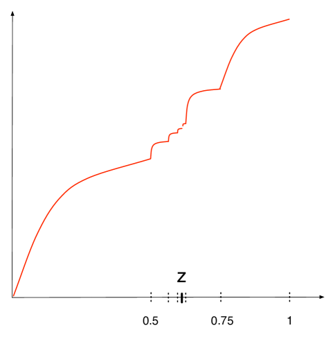
Figure 2. A function that is only dyadically differentiable at $z$

We now describe how to deal with the general situation. Our main technical concept is the following. For $p,q\in\mathbb{Q}$, $p>0$, we say that an interval is a $(p,q)$–interval if it is the image of a basic dyadic interval under the affine transformation $y\mapsto py+q$. Thus, a $(p,q)$–interval has the form

$$[pi2^{-n}+q,p(i+1)2^{-n}+q]$$

for some $i\in{\mathbb{Z}},n\in{\mathbb{N}}$.

We will show in Lemma 4.3 that there are rationals $p,q$ and $r,s$ such that

$$\liminf_{\begin{subarray}{c}|A|\to 0\\ A\ \text{is a}\ (r,s)-\text{interval}\\ z\in A\end{subarray}}S_{f}(A)\,\,<\limsup_{\begin{subarray}{c}|B|\to 0\\ B\ \text{is an}\ (p,q)-\text{interval}\\ z\in B\end{subarray}}S_{f}(B).$$ (9)

The strategy $\Gamma$ is in the betting state on $(p,q)$ intervals in the tree of intervals, and in the non-betting state on $(r,s)$–intervals. For each state, it proceeds exactly like the Doob strategy in the corresponding state. In addition, when $\Gamma$ switches state, the current interval is split into intervals of the other type (usually, into infinitely many intervals). Nonetheless, the other state takes effect immediately. So, in the betting state, we have to immediately bet on all the components of this (usually) infinite splitting.

4.1.3. The algebraic part.

We derive Lemma 4.3 from an algebraic lemma. For a set $L$ of rationals, an interval is called an $L$–interval if it is a $(p,q)$–interval for some $p,q\in L$.

Lemma 4.2.

For each rational $\alpha>1$, we can effectively determine a finite set $L$ of rationals in $[-1,1]$ such that for each interval $[x,y]$, $0<x<y<1$, there are $L$–intervals $A,B$ as follows:

$$[x,y]\subset A \& \frac{|A|}{y-x}<\alpha,$$

$$B\subset[x,y] \& \frac{y-x}{|B|}<\alpha.$$

Informally, we can approximate the given interval from the outside and from the inside by $L$–intervals within a “precision factor” of $\alpha$. We defer the proof of the lemma to Subsection 4.3.

By the hypothesis that $f^{\prime}(z)$ does not exist and Lemma 2.5, we can choose rationals $\widetilde{\beta}<\widetilde{\gamma}$ such that

$$\widetilde{\gamma} < \lim_{h\rightarrow 0}\sup\{S_{f}(x,y)\colon\,0\leq y-x\leq h\ \&\ z\in(x,y)\},$$

$$\widetilde{\beta} > \lim_{h\rightarrow 0}\inf\{S_{f}(x,y)\colon\,0\leq y-x\leq h\ \&\ z\in\text{ middle third of}\ (x,y)\}$$

Let $\alpha,\beta,\gamma$ be rationals such that $1<\alpha<\frac{4}{3}$ and

$\widetilde{\beta}\alpha<\beta<\gamma<\widetilde{\gamma}/\alpha$.

Lemma 4.3.

There are rationals $p,q$, $r,s$, such that $p,r>0$ and

$$\gamma < \lim_{h\rightarrow 0}\sup\{S_{f}(A)\colon\,A\ \text{is a}\ (p,q)\text{--interval}\ \&\ |A|\leq h\ \&\ z\in A\},$$

$$\beta > \lim_{h\rightarrow 0}\inf\{S_{f}(B)\colon\,B\ \text{is an}\ (r,s)\text{--interval}\ \&\ |B|\leq h\ \&\ z\in B\}.$$

Proof.

Let $L$ be as in Lemma 4.2. For the first inequality, we use the first line in Lemma 4.2.

Let $h>0$ be given. Choose reals $x<y$, where $x\leq z\leq y$, such that $y-x<h/\alpha$ and $S_{f}(x,y)>\widetilde{\gamma}$. By Lemma 4.2 there is an $L$–interval $A=[u,v]$ such that $[x,y]\subseteq A$ and $|A|/(y-x)<\alpha$. Then, since $f$ is nondecreasing and $v-u<\alpha(y-x)$, we have

$$S_{f}(A)=\frac{f(v)-f(u)}{v-u}\geq\frac{f(y)-f(x)}{v-u}>\frac{f(y)-f(x)}{(y-x)\alpha}>\widetilde{\gamma}/\alpha>\gamma.$$

Since $L$ is finite, we can now pick a single pair of rationals $p,q\in L$ which works for arbitrary small $h>0$, as required.

For the second inequality, the argument is similar, based on the second line in Lemma 4.2. However, we also need the condition on middle thirds in the definition of $\widetilde{\beta}$, because when we replace an interval $[x,y]$ by a subinterval $B$ that is an $(r,s)$-interval, we want to ensure that $z\in B$.

Given $h>0$, choose reals $x<y$, where $x\leq z\leq y$ and $z$ is in the middle third of $[x,y]$, such that $y-x<h/\alpha$ and $S_{f}(x,y)<\widetilde{\beta}$. By Lemma 4.2 there is an $L$–interval $B=[u,v]$ such that $B\subseteq[x,y]$ and $(y-x)/|B|<\alpha$. Since $\alpha<4/3$ and $z$ is in the middle third of $[x,y]$, we have $z\in B$. Similar to the estimates above, we have

$$S_{f}(B)\leq\frac{f(y)-f(x)}{v-u}\leq\frac{f(y)-f(x)}{(y-x)/\alpha}=\alpha S_{f}(x,y)<\alpha\widetilde{\beta}<\beta.\qed$$

4.1.4. Definition of $g$ on a dense set, and the strategy $\Gamma$

In the following fix $p,q,r,s$ as in Lemma 4.3. Recall that we plan to define an infinitely branching tree of intervals, and that, on each node $A$ in this tree, the strategy is either

• in a betting state, betting on smaller and smaller $(p,q)$–sub-intervals of $A$, or

• in a non-betting state, processing smaller and smaller $(r,s)$–sub-intervals of $A$, but without betting.

The root of the tree is $A=[0,1]$. Initially let $g(0)=0$ and $g(1)=1$ (hence $\Gamma(A)=1$), and put the strategy $\Gamma$ into the betting state.

One technical problem is that we never know a computable real such as $S_{f}(A)$ in its entirety; we only have rational approximations. For a real $x$ named by a Cauchy sequence as in Subsection 2.1, we let $x_{n}$ denote the $n$-th term of that sequence. Thus $|x-x_{n}|\leq 2^{-n}$. To make use of the inequalities in Lemma 4.3, we choose $K\in{\mathbb{N}}$ large enough that the inequalities still hold with $\gamma+2^{-K}$ instead of $\gamma$, and with $\beta-2^{-K}$ instead of $\beta$, respectively. We also require that $\beta+2^{-K}<\gamma-2^{-K}$.

Suppose $A=[a,b]$ is an interval such that $\Gamma(A)$ has already been defined. By hypothesis $S_{f}(A)$ is a computable real uniformly in $A$. Proceed according to the case that applies.

(I): $\Gamma$ is in the betting state on $A$.

(I.a) $S_{f}(A)_{K}\leq\gamma$. If $\Gamma$ has just entered the betting state on $A$, let

$A=\bigsqcup_{k}A_{k}$

where the $A_{k}$ form an effective sequence of $(p,q)$–intervals that are disjoint (on $[0,1]\setminus\mathbb{Q}$). Otherwise, split $A=A_{0}\cup A_{1}$ into disjoint intervals of equal length.

The function $g$ interpolates between $a$ and $b$ with a growth proportional to the growth of $f$: if $v\in(a,b)$ is an endpoint of a new interval, define

$$g(v)=g(a)+(g(b)-g(a))\frac{f(v)-f(a)}{f(b)-f(a)}.$$

Continue the strategy on each sub-interval.

(I.b) $S_{f}(A)_{K}>\gamma$. Switch to the non-betting state on $A$ and goto (II).

(II) $\Gamma$ is in the non-betting state on $A$.

(II.a) $S_{f}(A)_{K}\geq\beta$. If $\Gamma$ has just entered the non-betting state on $A$, let

$A=\bigsqcup_{k}A_{k}$

where the $A_{k}$ form an effective sequence of $(r,s)$–intervals that are disjoint on $[0,1]\setminus\mathbb{Q}$, and further, $2|A_{k}|\leq|A|$ for each $k$. Otherwise split $A=A_{0}\cup A_{1}$ into disjoint intervals of equal length.

If $v\in(a,b)$ is an endpoint of a new interval, then $g$ interpolates linearly: let

$$g(v)=g(a)+(g(b)-g(a))\frac{v-a}{b-a}.$$

Continue the strategy on each sub-interval.

(II.b) $S_{f}(A)_{K}<\beta$. Switch to the betting state on $A$ and goto (I).

4.1.5. The verification.

If the strategy $\Gamma$, processing an interval $A=[a,b]$ in the betting state, chooses a sub-interval $[c,d]$, then

$$g(d)-g(c)=(g(b)-g(a))\frac{f(d)-f(c)}{f(b)-f(a)}.$$

Dividing this equation by $d-c$ and recalling the definition of the $\Gamma$-values in (8), we obtain

$$\Gamma([c,d])=\Gamma([a,b])\frac{S_{f}(c,d)}{S_{f}(a,b)}.$$ (10)

The purpose of the following two claims is to extend $g$ to a computable function on $[0,1]$. For the rest of the proof, we will use the shorthand

$g[A]=g(b)-g(a)$

for an interval on the tree $A=[a,b]$. Recall that we write $S_{g}(A)$ for the slope $S_{g}(a,b)$. Thus $\Gamma(A)=S_{g}(A)=g[A]/|A|$.

Claim 4.4.

Let $x\in[0,1]$. Let $B_{0}\supset B_{1}\supset\cdots$ be an infinite path on the tree of intervals. Then $\lim_{m}g[B_{m}]=0$.

We consider the states of the betting strategy $\Gamma$ as it processes the intervals $A=B_{m}$.

Case 1: $\Gamma$ changes its state only finitely often when processing the intervals $B_{m}$.

If $\Gamma$ is eventually in a non-betting state then clearly $\lim_{m}g[B_{m}]=0$. Suppose otherwise, that is, $\Gamma$ is eventually in a betting state. Suppose further that $\Gamma$ enters the betting state for the last time when it defines the interval $A=B_{m^{*}}$. Then for all $m\geq m^{*}$, by (10) and since $S_{f}(B_{m})_{K}\leq\gamma$, we have

$$\Gamma(B_{m})=\Gamma(B_{m^{*}})\frac{S_{f}(B_{m})}{S_{f}(B_{m^{*}})}\leq(\gamma+2^{-K})\frac{\Gamma(B_{m^{*}})}{S_{f}(B_{m^{*}})}=:C.$$

Hence $g[B_{m}]=\Gamma(B_{m})\cdot|B_{m}|\leq C|B_{m}|$.

Case 2: $\Gamma$ changes its state infinitely often when processing the intervals $B_{m}$.

Let $B_{m_{i}}$ be the interval $A$ processed when the strategy is for the $i$-th time in a betting state at (I.b). Note that $g[B_{m_{i}+1}]\leq g[B_{m_{i}}]/2$ because at (II.a) we chose all the splitting components $A_{k}$ at most half as long as the given interval $A$. Of course, by monotonicity of $g$ we have $g[B_{m+1}]\leq g[B_{m}]$ for each $m$. Thus, $g[B_{m}]\leq 2^{-i}$ for each $m>m_{i}$. This completes the proof of the claim.

Claim 4.5.

The function $g$ can be extended to a computable function on $[0,1]$.

Let $V$ be the set of endpoints of intervals on the tree. Clearly $V$ is dense in $[0,1]$. For $x\in[0,1]$ let

$$\underline{g}(x) = \sup\{g(v)\colon\,v<x,v\in V\}$$

$$\overline{g}(x) = \inf\{g(w)\colon\,w>x,w\in V\}.$$

We show that $\underline{g}(x)\geq\overline{g}(x)$. Since $g$ is nondecreasing on $V$, this will imply that $\underline{g}=\overline{g}$ is a continuous extension of $g$.

There is an infinite path $B_{0}\supset B_{1}\supset\cdots$ on the tree of intervals such that $x\in\bigcap_{m}B_{m}$. By Claim 4.4, we have

$\underline{g}(x)\geq\sup_{m}g(\min\,B_{m})=\inf_{m}g(\max\,B_{m})\geq\overline{g}(x)$.

Clearly there is a computable dense sequence of rationals $\{v_{i}\}_{i\in{\mathbb{N}}}$ that lists without repetition the set $V$ of endpoints of intervals in the tree. By definition, $g(v_{i})$ is a computable real uniformly in $i$. Since $\underline{g}$ is continuous nondecreasing, by Proposition 2.2 we may conclude that $\underline{g}$ is computable. This establishes the claim.

From now on we will use the letter $g$ to denote the function extended to $[0,1]$.

Claim 4.6.

We have $\overline{D}g(z)=\infty$.

Let $\mathcal{C}$ denote the tree of intervals built during the construction. Note that for each $\epsilon>0$ there are only finitely many intervals in $\mathcal{C}$ of length greater than $\epsilon$. To prove the claim, we show that the strategy $\Gamma$ succeeds on $z$ in the sense that

$\sup_{z\in A\in\mathcal{C}}\Gamma(A)=\infty$.

By the definition of the $\Gamma$-values in (8) this will imply $\overline{D}g(z)=\infty$: let $([a_{n},b_{n}])_{n\in{\mathbb{N}}}$ be a sequence of intervals containing $z$ such that $\Gamma([a_{n},b_{n}])=S_{g}(a_{n},b_{n})$ is unbounded and $\lim_{n}(b_{n}-a_{n})=0$. If $z\in V$, then necessarily $a_{n}=z$ or $b_{n}=z$ for almost all $n$. This clearly implies $\overline{D}g(z)=\infty$. If $z\not\in V$, then $a_{n},b_{n}\neq z$ for all $n$, and we have $S_{g}(a_{n},b_{n})\leq\max\{S_{g}(a_{n},z),S_{g}(z,b_{n})\}$ by Fact 2.4. This also implies that $\overline{D}g(z)=\infty$.

Now we come to the crucial argument why $\Gamma$ succeeds, first we verify that $\Gamma$ changes its state infinitely often on intervals $B$ such that $z\in B$. Suppose $\Gamma$ entered the betting state in (II.b) and hence jumps to (I.a). Following the notation in (I.a), let $A_{k}$ be the $(p,q)$–interval containing $z$. By the first line in Lemma 4.3 and the definition of $K$ in 4.1.4, there is a $(p,q)$–interval $A\subseteq A_{k}$ containing $z$ such that $S_{f}(A)>\gamma+2^{-K}$. Thus $S_{f}(A)_{K}>\gamma$ and $\Gamma$ enters the non-betting state when it processes this interval, if not before.

Similarly, once $\Gamma$ enters the non-betting state on an interval $A_{k}$ containing $z$, by the second line of Lemma 4.3 it will revert to the betting state on some $(r,s)$–interval $B\subseteq A_{k}$ containing $z$.

Now suppose $\Gamma$ enters the betting state on $A$, $B$ is a largest sub-interval of $A$ such that $\Gamma$ enters the non-betting state on $B$, and then again, $C$ is a largest sub-interval of $B$ such that $\Gamma$ enters the betting state on $C$. Then $S_{f}(A)_{K}<\beta$ while $S_{f}(B)_{K}>\gamma$, so $\Gamma(B)=\Gamma(A)S_{f}(B)/S_{f}(A)\geq\Gamma(A)\delta$ with $\delta=\frac{\gamma-2^{-K}}{\beta+2^{-K}}>1$. Also $\Gamma(B)=\Gamma(C)$. Thus, after the strategy has entered the betting state for $n+1$ times on intervals containing $z$, we have $\Gamma(A)\geq\delta^{n}$. This implies that $\Gamma$ succeeds on $z$.

Remark 4.7.

Suppose we are given a computable function $f$ as in Theorem 4.1 by an index in the sense of Subsection 2.2. The method of the foregoing proof enables us to uniformly obtain an index for a computable nondecreasing function $p$ such that $f^{\prime}(z)\uparrow$ implies $\overline{D}p(z)=\infty$ for all $z\in[0,1]$. We simply sum up all the possibilities for $g$. This list of possibilities is effectively given: we have $f$ itself (for the case that already $\underline{D}f(z)=\infty$), and all the functions $g$ obtained for any possible values of the rationals $p,q,r,s$ and $0\leq\beta<\gamma$ in the construction above.

4.2. Proof of (i)$\to$(iii)

Suppose $\overline{D}g(z)=\infty$ where $g\colon\,[0,1]\rightarrow\mathbb{R}$ is a computable nondecreasing function. We may assume that $z$ is irrational. We want to show that $z$ is not computably random. We apply Lemma 4.2 for some fixed $\alpha>1$, obtaining a finite set $L\subseteq[-1,1]$ of rationals. There are $p,q$ in $L$, $p>0$, such that

$$\infty=\sup\{S_{g}(A)\colon\,A\ \text{is a}\ (p,q)\text{--interval}\ \&\ z\in A\}.$$ (11)

For a binary string $\sigma$, recall that $[\sigma]$ is the closed basic dyadic interval determined by $\sigma$. Let

$A_{\sigma}=p[\sigma]+q$.

We may assume that the given computable nondecreasing function $g$ is actually defined on $[-1,2]$, so that $S_{g}(A_{\sigma})$ is defined for each $\sigma$. To do so we let $g(x)=g(0)$ for $x\in[-1,0]$ and $g(x)=g(1)$ for $x\in[1,2]$ and note that this extended function is computable by Proposition 2.2. We define a computable martingale $N$ by

$$N(\sigma)=S_{g}(A_{\sigma}).$$

Now let $w$ be the irrational number $(z-q)/p$. Then $N$ succeeds on the binary expansion of the fractional part $w-\lfloor w\rfloor$. For, given $c>0$, by (11) let $\sigma$ be a string such that $z\in A_{\sigma}$ and $S_{g}(A_{\sigma})\geq c$. Then $\sigma$ is an initial segment of the binary expansion of $w-\lfloor w\rfloor$ and $N(\sigma)\geq c$.

It follows from the base invariance of computable randomness proved in Theorem 3.7 that $z=wp+q$ is also not computably random. ∎

4.3. Proof of Lemma 4.2

We may assume that $0<x<y<1/2$. Let $k$ be an odd prime number such that $1+8/k<\alpha$. Let

$$P = \{l/k\colon\,l\in{\mathbb{N}}\ \&\ k/2<l\leq k\},$$

$$Q = \{v/k\colon\,v\in{\mathbb{Z}}\ \&\ |v|\leq k\}$$

We claim that

$L=P\cup PQ$

is a finite set of rationals as required. Informally speaking, $P$ is a set of scaling factors for intervals, and $PQ$ is a set of possible shifts for intervals.

Finding $A$. To obtain $A\supset[x,y]$, let $n\in{\mathbb{N}}$ be largest such that $y-x<(1-1/k)2^{-n}$, and let $\eta=1/(2^{n}k)$. Informally $\eta$ is the “resolution” for a discrete version of the picture that will suffice to find $A$ and $B$. By the definitions we have

$$y-x+\eta<2^{-n}.$$ (12)

Pick the least scaling factor $p\in P$ such that

$$y-x+\eta<p2^{-n}.$$ (13)

Note that $p>\min P$: if $p=\frac{k+1}{2k}$ then $y-x+\eta<p2^{-n}$ implies $y-x<(1-1/k)2^{-n-1}$ contrary to the maximality of $n$. Therefore we have

$$p2^{-n}\leq y-x+2\eta.$$ (14)

Let $M\in{\mathbb{N}}$ be greatest such that $M\eta<x/p$. Now comes the key step: since $k$ and $2^{n}$ are coprime, in the abelian group ${\mathbb{Q}}/{\mathbb{Z}}$, the elements $1/k$ and $1/2^{n}$ together generate the same cyclic group as $\eta$. Working still in ${\mathbb{Q}}/{\mathbb{Z}}$, there are $i,v_{0}\in{\mathbb{N}}$, $0\leq i<2^{n}$, $v_{0}\leq k$ such that $[i/2^{n}]+[v_{0}/k]=[M\eta]$. Then, since $M\eta\leq 1$, there is an integer $v$, $|v|\leq k$, such that

$$i/2^{n}+v/k=M\eta.$$ (15)

To define the $L$–interval $A$, let $q=v/k\in Q$. Let

$A=p[i2^{-n},(i+1)2^{-n}]+pq$.

Write $A=[a,b]$. We verify that $A$ is as required.

Firstly, $a=pi2^{-n}+pq=pM\eta<x$, and $x-a\leq p\eta\leq\eta$ because of the maximality of $M$ and because $p\leq 1$.

Secondly, $|A|=p2^{-n}$, so we have by (13) and (14) that $y<b<y+2\eta$. Then

$|A|\leq y-x+2\eta=y-x+2/(2^{n}k)\leq y-x+8(y-x)/k$,

where the last inequality holds because $2^{-n}\leq 4(y-x)$ by the maximality of $n$. Thus $|A|/(y-x)\leq 1+8/k<\alpha$, as required.

Finding $B$. Let $\alpha=1+2\epsilon$. The second statement of the lemma can be derived from the first statement for the precision factor $1+\epsilon$. Let $L$ be the finite set of rationals obtained in the first statement for $1+\epsilon$ in place of $\alpha$. Given an interval $[x,y]$, let $[u,v]\subseteq[x,y]$ be the sub-interval such that

$u-x=y-v=\epsilon(v-u)$.

By the first statement of the lemma there is an $L$–interval $B=[a,b]\supseteq[u,v]$ such that $|B|/(v-u)<1+\epsilon$. Then

$$u-a < \epsilon(v-u)=u-x$$

$$b-v < \epsilon(v-u)=y-v,$$

whence $B\subset[x,y]$. Clearly, $(y-x)/|B|<(y-x)/(v-u)=\alpha$.

Remark 4.8.

To illustrate the lemma and its proof, suppose $\alpha=4$. We can choose $k$ to be the prime $3$. This yields a set $L$ of at most 16 rationals. We have $P=\{\frac{2}{3},1\}$, but the proof shows that in order to find $A$ we never choose $p=\min P$. Thus $p=1$. The shift parameter $q$ is of the form $v/3$, where $v$ is an integer and $|v|\leq 3$. Thus, every interval $[x,y]$ is contained in a basic dyadic interval shifted by some $q$, and of length less than $4(y-x)$. A similar fact can be shown with the usual “1/3-trick”: the endpoints of a basic dyadic interval of length $2^{-m}$, and another basic dyadic interval shifted by $1/3$ and of the same length, are at least $2^{-m}/3$ apart.

5. Consequences of Theorem 4.1

In this section we provide some interesting consequences of Theorem 4.1 and its proof. We say that a real $z\in{\mathbb{R}}$ satisfies an algorithmic randomness notion if its fractional part $z-\lfloor z\rfloor$ satisfies it.

Corollary 5.1.

Each computable nondecreasing function $f$ is differentiable at a computable real. Moreover, the real can be obtained uniformly from an index for $f$.

Proof.

By Remark 4.7 above, from an index for $f$ we can compute an index for a nondecreasing function $g$ such that $f^{\prime}(z)\uparrow$ implies $\overline{D}g(z)=\infty$ for all $z\in[0,1]$. Our first goal is to show that one can compute an index for a function $h$ such that $\underline{D}h(z)=\infty$ in case $f^{\prime}(z)\uparrow$, for each $z\in[1/3,2/3)$. The idea is to turn appropriate martingales into martingales with the savings property, and then apply the implication (i)$\to$(ii) of Theorem 3.6.

We use the simple case of Lemma 4.2 with the parameters as in the foregoing Remark 4.8. Let $q$ range over rationals of the form $v/3$, where $v$ is an integer and $|v|\leq 3$.

Let $N_{q}$ be the computable martingale $N$ obtained in the proof of (i)$\to$ (iii) of Thm. 4.1 above for $p=1$. By Proposition 3.4 from an index for $N_{q}$ we can compute a martingale $M_{q}$ with the savings property that succeeds on the binary expansion of a real $u\in[0,1]$ if $N$ does.

Let $x$ range over $[1/3,2/3]$. For $x<2/3$ let $v_{q}(x)$ be the fractional part of $x-q$; let $v_{q}(2/3)=\lim_{x<2/3,x\to 2/3}v_{q}(x)$. Let $h_{q}(x)=\mbox{\rm{cdf}}(M_{q})(v_{q}(x))$, and let $h(x)=\sum_{q}h_{q}(x)$. Clearly $h$ is computable from an index for $f$.

Now consider $z\in[1/3,2/3)$ such that $f^{\prime}(z)\uparrow$. Then $\overline{D}g(z)=\infty$, so for some $q$, $N_{q}$ succeeds on the binary expansion of $v_{q}(z)$ as observed in the proof of (i)$\to$(iii) of Thm. 4.1. Hence $M_{q}$ succeeds on the binary expansion of $v_{q}(z)$, which by the implication (i)$\to$(ii) of Theorem 3.6 implies that $\underline{D}h_{q}(z)=\infty$. Therefore $\underline{D}h(z)=\infty$.

Let $r(x)=h(x)-h(1/3)$, extend this to a computable nondecreasing function on $[0,1]$ by assigning the value $0$ to $y<1/3$, and the value $h(2/3)$ to $y>2/3$, and let $V$ be the computable martingale $\mbox{\rm{mart}}(r)$. We have $\mbox{\rm{cdf}}(V)=r$ by Fact 3.5. By the implication (ii)$\to$(i) of Theorem 3.6 (which does not rely on the savings property), we may conclude that $V$ succeeds on the binary expansion of $z$. Note that an index for $V$, viewed as a function from binary strings to Cauchy names for reals, is computable from an index for $g$, and hence from an index for $f$.

It remains to compute, from an index for $V$, the binary expansion $Z$ of a real $z\in[1/3,2/3)$ such that $V(Z\!\upharpoonright_{n})$ is bounded. Let the first 3 bits of $Z$ be $1,0,0$. For $n\geq 3$, if $\sigma=Z\!\upharpoonright_{n}$ has been determined, use $V$ to determine a bit $Z(n)=b$ such that $V(\sigma\widehat{\ }b)\leq V(\sigma\widehat{\ }(1-b))+2^{-n}$. Clearly, $\sup_{n}V(Z\!\upharpoonright_{n})<\infty$. ∎

Note that in the argument above, different indices for $f$ might result in different reals. Next we obtain a preservation result for computable randomness. For instance, computable randomness is preserved under the map $z\mapsto e^{z}$, and, for each computable real $\alpha\neq 0$, under the map $z\mapsto z^{\alpha}$.

Corollary 5.2.

Suppose $z\in{\mathbb{R}}$ is computably random. Let $H$ be a computable function that is 1-1 in a neighborhood of $z$. If $H^{\prime}(z)\neq 0$, then $H(z)$ is computably random.

Proof.

Note that $H^{\prime}(z)$ exists by Theorem 4.1. First suppose $H$ is increasing in a neighborhood of $z$. If a function $f$ is computable and nondecreasing in a neighborhood of $H(z)$, then the composition $f\circ H$ is nondecreasing in a neighborhood of $z$. Thus, since $z$ is computably random, $(f\circ H)^{\prime}(z)$ exists. Since $H^{\prime}(z)\neq 0$, this implies that $f^{\prime}(H(z))$ exists. Hence $H(z)$ is computably random.

If $H$ is decreasing, we apply the foregoing argument to $-H$ instead. ∎

Corollary 5.3.

If a real $z\in[0,1]$ is computably random, then each computable Lipschitz function $h$ on the unit interval is differentiable at $z$.

Proof.

Suppose $h$ is Lipschitz via a constant $C\in{\mathbb{N}}$. Then the function $f$ given by $f(x)=Cx-h(x)$ is computable and nondecreasing. Thus, by (i)$\to$(ii) of Theorem 4.1, $f$ and hence $h$ is differentiable at $z$. ∎

The converse of Cor. 5.3 has been shown in [14]. Thus, monotonicity can be replaced by being Lipschitz in Theorem 4.1. Note that the function $f$ in the foregoing proof is Lipschitz. Thus, computable randomness is characterized by differentiability of computable functions that are monotonic, or Lipschitz, or both monotonic and Lipschitz. This accounts for some arrows in Figure 1 in the introduction.

5.1. The Denjoy alternative for computable functions

Several theorems in classical real analysis say that a certain function is well-behaved almost everywhere. Being well-behaved can mean other things than being differentiable, although it is usually closely related. In the next two subsections we give two examples of such results and discuss their effective versions. As before, $\mathbf{\lambda}$ denotes the usual Lebesgue measure on the unit interval.

The first result applies to arbitrary functions on the unit interval. For a somewhat more general Theorem, see [2, Thm. 5.8.12] or [4, 7:9.5].

Theorem 5.4 (Denjoy, Saks, Young).

Let $f$ be a function $[0,1]\rightarrow\mathbb{R}$. Then $\mathbf{\lambda}$-almost surely, the Denjoy alternative holds at $z$:

either $f^{\prime}(z)$ exists, or $\overline{D}f(z)=\infty$ and $\underline{D}f(z)=-\infty$.

The Denjoy alternative for effective functions was first studied by Demuth (see [16]). The following result is a combination of work by Demuth, Miller, Nies, and Kučera. In contrast to Theorem 4.1, it characterizes computable randomness in terms of a differentiability property of computable functions, without any additional conditions on the function.

Theorem 5.5.

Let $z\in[0,1]$. Then $z$ is computably random $\Leftrightarrow$

for every computable $f\colon\,[0,1]\to\mathbb{R}$ the Denjoy alternative holds at $z$.

Proof.

For the implication “$\Leftarrow$”, let $f$ be a nondecreasing computable function. Since $f$ satisfies the Denjoy alternative at $z$ and $\underline{D}f(z)\geq 0$, this means that $f^{\prime}(z)$ exists. Thus $z$ is computably random by Theorem 4.1.

For a proof of the implication “$\Rightarrow$” see [1]. ∎

5.2. The Lebesgue differentiation theorem and $\mathcal{L}_{1}$-computable functions

The following result is usually called the Lebesgue differentiation theorem. For a proof, see [2, Section 5.4].

Theorem 5.6.

Let $g\colon\,[0,1]\rightarrow\mathbb{R}$ be integrable. Then $\mathbf{\lambda}$-almost surely,

$$g(z)=\lim_{r\rightarrow 0}\frac{1}{r}\int_{z}^{z+r}g\,d\mathbf{\lambda}.$$

Before we discuss an effective version of this, we need some basics on $\mathcal{L}_{1}$-computable functions in the sense of [23, p. 84]. Recall that $\mathcal{L}_{1}([a,b])$ denotes the set of integrable functions $g:[a,b]\rightarrow\mathbb{R}$, and $||g||_{1}=\int_{[a,b]}|g|d\mathbf{\lambda}$. We say that $g:[0,1]\rightarrow\mathbb{R}$ is $\mathcal{L}_{1}$-computable if there is a uniformly computable sequence $(h_{n})_{n\in{\mathbb{N}}}$ of functions on $[0,1]$ such that $||g-h_{n}||_{1}\leq 2^{-n}$ for each $n$. (The notion of computability for the $h_{n}$ is the usual one in the sense of Subsection 2.2; in particular, they are continuous.)

For a function $h$, we let $h^{+}=\max(h,0)$ and $h^{-}=\max(-h,0)$. If $g$ is $\mathcal{L}_{1}$-computable via $(h_{n})_{n\in{\mathbb{N}}}$, then $g^{+}$ is $\mathcal{L}_{1}$-computable via $(h_{n}^{+})_{n\in{\mathbb{N}}}$, and $g^{-}$ is $\mathcal{L}_{1}$-computable via $(h_{n}^{-})_{n\in{\mathbb{N}}}$. (This follows because $|g^{+}(x)-h_{n}^{+}(x)|\leq|g(x)-h_{n}(x)|$, etc.)

If $g\in\mathcal{L}_{1}([0,1])$ then its restriction to the interval $[0,x]$ is in $\mathcal{L}_{1}([0,x])$. Let $G(x)=\int_{0}^{x}gd\mathbf{\lambda}$. We have $G=G^{+}-G^{-}$ where $G^{+}(x)=\int_{0}^{x}g^{+}d\mathbf{\lambda}$ and $G^{-}(x)=\int_{0}^{x}g^{-}d\mathbf{\lambda}$.

Fact 5.7.

If $g$ is $\mathcal{L}_{1}$-computable then $G^{+}$ and $G^{-}$ are computable.

Proof.

For each $\mathcal{L}_{1}$-computable function $f$, $\int_{0}^{q}fd\mathbf{\lambda}$ is computable uniformly in a rational $q$ by [22, Lemma 2.3]. Thus the nondecreasing continuous functions $G^{+},G^{-}$ are computable by Proposition 2.2. ∎

By Theorem 5.6, if $g$ is in $\mathcal{L}_{1}([0,1])$ and $G$ is as above, then for $\mathbf{\lambda}$-almost every $z$, $G^{\prime}(z)$ exists and equals $g(z)$. For the mere existence of $G^{\prime}(z)$, we have the following.

Corollary 5.8.

Let $g$ be $\mathcal{L}_{1}$-computable. Then $G^{\prime}(z)$ exists for each computably random real $z$.

Proof.

It suffices to note that by Fact 5.7 and Theorem 4.1, $(G^{+})^{\prime}(z)$ and $(G^{-})^{\prime}(z)$ exist. ∎

The condition in Cor. 5.8 that $G^{\prime}(z)$ exists for each $\mathcal{L}_{1}$-computable function $g$ actually characterizes Schnorr randomness by recent results of Rute [26], and Pathak, Rojas and Simpson already mentioned in the introduction.

6. Weak $2$-randomness and Martin-Löf randomness

In this section, when discussing inclusion, disjointness, etc., for open sets in the unit interval, we will ignore the elements that are dyadic rationals. For instance, we view the interval $(1/4,3/4)$ as the union of $(1/4,1/2)$ and $(1/2,3/4)$. With this convention, the clopen sets in Cantor space $2^{\omega}$ correspond to the finite unions of open intervals with dyadic rational endpoints.

6.1. Characterizing weak 2-randomness in terms of differentiability

Recall that a real $z$ is weakly $2$-random if $z$ is in no null $\Pi^{0}_{2}$ set.

Theorem 6.1.

Let $z\in[0,1]$. Then

$z$ is weakly $2$-random $\Leftrightarrow$

each a.e. differentiable computable function is differentiable at $z$.

Proof.

“$\Rightarrow$”: For rationals $p,q$ let

$$\underline{C}(p) = \{z\colon\,\forall t>0\,\exists h\,\big{[}0<|h|\leq t\ \&\ \,S_{f}(z,z+h)<p\big{]}\}$$

$$\overline{C}(q) = \{z\colon\,\forall t>0\,\exists h\,\big{[}0<|h|\leq t\ \&\ \,S_{f}(z,z+h)>q\big{]}\},$$

where $t,h$ range over rationals. The function $z\mapsto S_{f}(z,z+h)$ is computable, and its index in the sense of Subsection 2.2 can be obtained uniformly in $h$. Hence the set

$\{z\colon S_{f}(z,z+h)<p\}$

is a $\Sigma^{0}_{1}$ set uniformly in $p,h$ by Lemma 2.3 and its uniformity in the strong form remarked after its proof. Thus $\underline{C}(p)$ is a $\Pi^{0}_{2}$ set uniformly in $p$. Similarly, $\overline{C}(q)$ is a $\Pi^{0}_{2}$ set uniformly in $q$. Clearly,

$\underline{D}f(z)<p$	$\Rightarrow$	$z\in\underline{C}(p)$	$\Rightarrow$	$\underline{D}f(z)\leq p$,
$\overline{D}f(z)>q$	$\Rightarrow$	$z\in\overline{C}(q)$	$\Rightarrow$	$\overline{D}f(z)\geq q$.

Therefore $f^{\prime}(z)$ fails to exist iff

$$\forall p\,[\,z\in\underline{C}(p)]\ \vee\ \forall q\,[\,z\in\overline{C}(q)]\ \vee\ \exists p\exists q[p<q\ \&\ z\in\underline{C}(p)\ \&\ z\in\overline{C}(q)],$$

where $p,q$ range over rationals. This shows that $\{z\colon\,f^{\prime}(z)\ \text{fails to exist}\}$ is a $\Sigma^{0}_{3}$ set (i.e., an effective union of $\Pi^{0}_{2}$ sets). If $f$ is a.e. differentiable then this set is null and thus cannot contain a weakly $2$-random.

“$\Leftarrow$”: For an interval $A\subseteq[0,1]$ and $p\in{\mathbb{N}}$ let $\Lambda_{A,p}$ be the “sawtooth function” that is constant 0 outside $A$, reaches $p|A|/2$ at the middle point of $A$ and is linearly interpolated elsewhere. Thus $\Lambda_{A,p}$ has slope $\pm p$ between pairs of points in the same half of $A$, and

$$\Lambda_{A,p}(x)\leq p|A|/2,$$ (16)

for each $x$.

Let $(\mathcal{G}_{m})_{m\in{\mathbb{N}}}$ be a sequence of uniformly $\Sigma^{0}_{1}$ sets in the sense of Subsection 2.4, where $\mathcal{G}_{m}\subseteq[0,1]$, such that $\mathcal{G}_{m}\supseteq\mathcal{G}_{m+1}$ for each $m$. We build a computable function $f$ such that $f^{\prime}(z)$ fails to exist for every $z\in\bigcap_{m}\mathcal{G}_{m}$. To establish the implication $\Leftarrow$, we also show in Claim 6.4 that the function $f$ is a.e. differentiable in the case that $\bigcap_{m}\mathcal{G}_{m}$ is null.

Recall the convention that we ignore the dyadic rationals when discussing inclusion, union, disjointness, etc., for open sets in the unit interval. We have an effective enumeration $(D_{m,l})_{m,l\in{\mathbb{N}}}$ of open intervals with dyadic rational endpoints such that

$\mathcal{G}_{m}=\bigsqcup_{l\in{\mathbb{N}}}D_{m,l},$

for each $m$ (the symbol $\bigsqcup$ indicates a disjoint union). We may assume, without loss of generality, that for each $m,k$, there is an $l$ such that $D_{m+1,k}\subseteq D_{m,l}$.

We construct by recursion on $m$ a computable double sequence $(C_{m,i})_{m,i\in{\mathbb{N}}}$ of open intervals with dyadic rational endpoints such that $\bigsqcup_{i}C_{m,i}=\mathcal{G}_{m}$,

$$C_{m,i}\cap C_{m,k}=\emptyset\ \text{and}\ |C_{m,i}|\geq|C_{m,k}|\ \text{for}\ i<k,$$ (17)

and, furthermore, if $B=C_{m,i}$ for $m>0$, then there is an interval $A=C_{m-1,k}$ such that

$$B\subseteq A\ \&\ |B|\leq 8^{-m}|A|.$$ (18)

Each interval of the form $D_{m,k}$ will be a finite union of intervals of the form $C_{m,i}$.

Construction of the double sequence $(C_{m,i})_{m,i\in{\mathbb{N}}}$.

Suppose $m=0$, or $m>0$ and we have already defined $(C_{m-1,j})_{j\in{\mathbb{N}}}$. Define $(C_{m,i})_{i\in{\mathbb{N}}}$ as follows.

Suppose $N\in{\mathbb{N}}$ is greatest such that we have already defined $C_{m,i}$ for $i<N$. When a new interval $D=D_{m,l}$ with dyadic rational endpoints is enumerated into $\mathcal{G}_{m}$, if $m>0$ we wait until $D$ is contained in a union of intervals $\bigcup_{r\in F}C_{m-1,r}$, where $F$ is finite. This is possible because $D$ is contained in a single interval in $\mathcal{G}_{m-1}$, and this single interval was handled in the previous stage of the recursion. If $m>0$, let $\delta$ be the minimum of $|D|$ and the lengths of these finitely many intervals; if $m=0$, let $\delta=|D|$. Let $\epsilon$ be the minimum of $|C_{m,N-1}|$ (if $N>0$), and $8^{-m}2^{-l}\delta$. (We will need the factor $2^{-l}$ when we show in Claim 6.4 that $f$ is a.e. differentiable.)

We partition $D$ into disjoint sub-intervals $C_{m,i}$ with dyadic rational endpoints, $i=N,\ldots,N^{\prime}-1$, and of nonincreasing length at most $\epsilon$, so that in case $m>0$ each of the sub-intervals is contained in an interval $A$ of the form $C_{m-1,r}$ for some $r\in F$. For $m\in{\mathbb{N}}$ let

$$f_{m}=\sum_{i=0}^{\infty}\Lambda_{C_{m,i},4^{m}},$$

and let $f=\sum_{m=0}^{\infty}f_{m}$. Since $|C_{m,i}|\leq 8^{-m}$ for each $i$, we have $f_{m}(x)\leq 8^{-m}4^{m}/2\leq 2^{-m-1}$ for each $x$.

Claim 6.2.

The function $f$ is computable.

Since $f_{m}(x)\leq 2^{-m-1}$ for each $m$, $f(x)$ is defined for each $x\in[0,1]$. We first show that $f(q)$ is computable uniformly in a rational $q$. Given $m>0$, since $|C_{m,i}|\to_{i}0$, we can find $i^{*}$ such that

$|C_{k,i^{*}}|\leq 8^{-m}/(m+1)$ for each $k\leq m$.

Then, since the length of the intervals $C_{k,i}$ is nonincreasing in $i$ and by (16), we have $\Lambda_{C_{k,i},4^{k}}(q)\leq 2^{-m-1}/(m+1)$ for all $k\leq m$ and $i\geq i^{*}$. So by the disjointness in (17), $\sum_{k\leq m}\sum_{i\geq i^{*}}\Lambda_{C_{k,i},4^{k}}(q)\leq 2^{-m-1}$. We also have $\sum_{k>m}f_{k}(q)\leq\sum_{k>m}2^{-k-1}=2^{-m-1}$. Hence the approximation to $f(q)$ at stage $i^{*}$ based only on the intervals of the form $C_{k,i}$ for $k\leq m$ and $i<i^{*}$ is within $2^{-m}$ of $f(q)$.

To show $f$ is computable, by Subsection 2.2 it suffices now to verify that $f$ is effectively uniformly continuous. Suppose $|x-y|\leq 8^{-m}$. For $k<m$, we have $|f_{k}(x)-f_{k}(y)|\leq 4^{k}|x-y|$. For $k\geq m$ we have $f_{k}(x),f_{k}(y)\leq 2^{-k-1}$. Thus

$$|f(x)-f(y)|\leq|x-y|\sum_{k<m}4^{k}+\sum_{k\geq m}2^{-k}<2^{-m+2}.$$

Claim 6.3.

Suppose $z\in\bigcap\mathcal{G}_{m}$. Then $\overline{D}f(z)=\infty$ or $\underline{D}f(z)=-\infty$.

For each $m$ there is an interval $A_{m}$ of the form $C_{m,i}$ such that $z\in A_{m}$. Suppose first that there are infinitely many $m$ such that $z$ is in the left half of $A_{m}$. We show $\overline{D}f(z)=\infty$. Let $m$ be one such value. Choose

$$h=\pm|A_{m}|/4$$

so that $z+h$ is also in the left half of $A_{m}$. We show that the slope

$S_{f_{m}}(z,z+h)=4^{m}$

does not cancel out with the slopes, possibly negative, that are due to other $f_{k}$. If $k<m$ then we have $|S_{f_{k}}(z,z+h)|\leq 4^{k}$. Suppose $k>m$. Then by (16) and (18) we have $f_{k}(x)\leq 4^{k}8^{-k}|A_{m}|/2=2^{-k-1}|A_{m}|$ for $x\in\{z,z+h\}$ and hence

$$|S_{f_{k}}(z,z+h)|\leq\frac{2^{-k}|A_{m}|}{|h|}=2^{-k+2}.$$

Therefore, for $m>0$

$$S_{f}(z,z+h)\geq 4^{m}-\sum_{k<m}4^{k}-\sum_{k>m}2^{-k+2}\geq 4^{m-1}-4.$$

Thus $\overline{D}f(z)=\infty$.

If there are infinitely many $m$ such that $z$ is in the right half of $A_{m}$, then $\underline{D}f(z)=-\infty$ by a similar argument.

Claim 6.4.

If $\bigcap_{m}{\mathcal{G}}_{m}$ is null, then $f$ is differentiable almost everywhere.

Let $\widehat{D}_{m,l}$ be the open interval in $\mathbb{R}$ with the same middle point as $D_{m,l}$ such that $|\widehat{D}_{m,l}|=3|D_{m,l}|$. Let $\widehat{\mathcal{G}}_{m}=[0,1]\cap\bigcup_{l}\widehat{D}_{m,l}$. Clearly $\mathbf{\lambda}\widehat{\mathcal{G}}_{m}\leq 3\mathbf{\lambda}\mathcal{G}_{m}$, so that $\bigcap_{m}\widehat{\mathcal{G}}_{m}$ is null.

We show that $f^{\prime}(z)$ exists for each $z\not\in\bigcap_{m}\widehat{\mathcal{G}}_{m}$ that is not a dyadic rational. In the following, let $h,h_{0}$, etc., range over rationals. Note that

$S_{f}(z,z+h)=\sum_{k=0}^{\infty}S_{f_{k}}(z,z+h)$.

Let $m$ be the least number such that $z\not\in\widehat{\mathcal{G}}_{m}$. Since $z$ is not a dyadic rational, we may choose $h_{0}>0$ such that for each $k<m$, the function $f_{k}$ is linear in the interval $[z-h_{0},z+h_{0}]$. So for $|h|\leq h_{0}$ the contribution of these $f_{k}$ to the slope $S_{f}(z,z+h)$ is constant. It now suffices to show that

$\lim_{h\to 0}\sum_{r=m}^{\infty}|S_{f_{r}}(z,z+h)|=0$.

Note that $f_{r}$ is nonnegative and $f_{r}(z)=0$ for $r\geq m$. Thus it suffices, given $\epsilon>0$, to find a positive $h_{1}\leq h_{0}$ such that

$$\sum_{r=m}^{\infty}f_{r}(z+h)\leq\epsilon|h|$$ (19)

whenever $|h|\leq h_{1}$.

Roughly, the idea is the following: take $r\geq m$. If $f_{r}(z+h)\neq 0$ then $z+h$ is in some $D_{m,l}$. Because $z\not\in\widehat{D}_{m,l}$, $|h|\geq|D_{m,l}|$. We make sure that $f_{r}(z+h)$ is small compared to $|h|$ by using that the height of the relevant sawtooth depends on the length of its base interval $C_{r,v}$ containing $z+h$, and that this length is small compared to $h$.

We now provide the details on how to find $h_{1}$ as above. Choose $l^{*}\in{\mathbb{N}}$ such that $2^{-l^{*}}\leq\epsilon$. If $C_{m,i}\subseteq D_{m,l}$ and $l\geq l^{*}$, we have

$$|C_{m,i}|\leq 8^{-m}\epsilon|D_{m,l}|.$$ (20)

Let $h_{1}=\min\{|D_{m,l}|\colon\,{l<l^{*}}\}$. Suppose $h>0$ and $|h|\leq h_{1}$.

Firstly we consider the contribution of $f_{m}$ to (19). If $f_{m}(z+h)>0$ then $z+h\in C_{m,i}\subseteq D_{m,l}$ for some (unique) $l,i$. Since $z\not\in\widehat{D}_{m,l}$ and $|h|\leq h_{1}$, we have $|h|\geq|D_{m,l}|$ and $l\geq l^{*}$. By (16), (20) and the definition of $f_{m}$,

$f_{m}(z+h)\leq 4^{m}|C_{m,i}|/2\leq 2^{-m-1}|D_{m,l}|\epsilon$.

Thus $f_{m}(z+h)\leq 2^{-m-1}\epsilon|h|$.

Next, we consider the contribution of $f_{r}$, $r>m$, to (19). If $f_{r}(z+h)>0$ then $z+h\in C_{r,v}\subseteq C_{m,i}$ for some $v$. Thus, by construction,

$f_{r}(z+h)\leq 4^{r}|C_{r,v}|/2\leq 4^{r}8^{-r}|C_{m,i}|/2\leq 2^{-r-1}|D_{m,l}|\epsilon\leq 2^{-r-1}\epsilon|h|$.

This establishes (19) and completes the proof. ∎

6.2. Characterizing Martin-Löf randomness in terms of differentiability

Recall that a function $f\colon\,[0,1]\rightarrow\mathbb{R}$ is of bounded variation if

$$\infty>\sup\sum_{i=1}^{n}|f(t_{i+1})-f(t_{i})|,$$

where the sup is taken over all collections $t_{1}<t_{2}<\ldots<t_{n}$ in $[0,1]$. A stronger condition on $f$ is absolute continuity: for every $\epsilon>0$, there is $\delta>0$ such that

$$\epsilon>\sup\sum_{i=1}^{n}|f(b_{i})-f(a_{i})|,$$

for every collection $0\leq a_{1}<b_{1}\leq a_{2}<b_{2}\leq\ldots\leq a_{n}<b_{n}\leq 1$ such that $\delta>\sum_{i=1}^{n}b_{i}-a_{i}$. The absolutely continuous functions are precisely the indefinite integrals of functions in $\mathcal{L}_{1}([0,1])$ (see [2, Thm. 5.3.6]). Note that it is easy to construct a computable differentiable function that is not of bounded variation.

We will characterize Martin-Löf randomness via differentiability of computable functions of bounded variation, following the scheme $(*)$ in the introduction. For the implication $\Leftarrow$, an appropriate single function suffices, because there is a universal Martin-Löf test.

Lemma 6.5 ([7], Example 2).

There is a computable function $f$ of bounded variation (in fact, absolutely continuous) such that $f^{\prime}(z)$ exists only for Martin-Löf random reals $z$.

Proof.

Let $(\mathcal{G}_{m})_{m\in{\mathbb{N}}}$ be a universal Martin-Löf test, where $\mathcal{G}_{m}\subseteq[0,1]$, such that $\mathcal{G}_{m}\supseteq\mathcal{G}_{m+1}$ for each $m$. We may assume that $\mathbf{\lambda}\mathcal{G}_{m}\leq 8^{-m}$. Define a computable function $f$ as in the proof of the implication $\Leftarrow$ of Theorem 6.1. By Claim 6.3, $f^{\prime}(z)$ fails to exist for any $z\in\bigcap_{m}\mathcal{G}_{m}$, i.e., for any $z$ that is not Martin-Löf random. It remains to show the following.

Claim 6.6.

$f$ is absolutely continuous, and hence of bounded variation.

For an open interval $A\subseteq[0,1]$, let $\Theta_{A,p}$ be the function that is undefined at the endpoints and the middle point of $A$, has value $p$ on the left half, value $-p$ on the right half of $A$, and is $0$ outside $A$. Then $\int_{0}^{x}\Theta_{A,p}=\Lambda_{A,p}(x)$.

Let $g_{m}=\sum_{i}\Theta_{C_{m,i},4^{m}}$. Note that $\mathbf{\lambda}\mathcal{G}_{m}\leq 8^{-m}$ implies that $g_{m}$ is integrable with $\int|g_{m}|\leq 2^{-m}$, and hence $\sum_{m}\int|g_{m}|\leq 2$. Then, by a well-known corollary to the Lebesgue dominated convergence theorem (see for instance [25, Thm. 1.38]), the function $g(y)=\sum_{m}g_{m}(y)$ is defined a.e., $g$ is integrable, and $\int_{0}^{x}g=\sum_{m}\int_{0}^{x}g_{m}$. Since $f_{m}(x)=\int_{0}^{x}g_{m}$, this implies that $f(x)=\int_{0}^{x}g$. Thus, $f$ is absolutely continuous. ∎

For a function $h$, let $h^{+}=\max(h,0)$ and $h^{-}=\max(-h,0)$, so that $h=h^{+}-h^{-}$. Since $g^{+}=\sum_{m}g_{m}^{+}$ and $g^{-}=\sum_{m}g_{m}^{-}$, by the monotone convergence theorem (see for instance [2, Thm. 2.8.2]), we have

$\int_{0}^{x}g^{+}=\sum_{m}\int_{0}^{x}g_{m}^{+}$ and $\int_{0}^{x}g^{-}=\sum_{m}\int_{0}^{x}g_{m}^{-}$.

Since $\mathbf{\lambda}\mathcal{G}_{m}\leq 8^{-m}$, we have $\int_{0}^{x}g_{m}^{+}\leq 2^{-m}$ and $\int_{0}^{x}g_{m}^{-}\leq 2^{-m}$, so both sums above are bounded by $2$. Hence the function $g$ is integrable with $\int_{0}^{x}g=\int_{0}^{x}g^{+}-\int_{0}^{x}g^{-}=f(x)$.

We now arrive at the analytic characterization of Martin-Löf randomness originally due to Demuth [7]. The implication (i)$\rightarrow$(ii) below restates [7, Thm. 3] in classical language.

Theorem 6.7.

The following are equivalent for $z\in[0,1]$:

• $z$ is Martin-Löf random.

• Every computable function $f$ of bounded variation is differentiable at $z$.

• Every computable function $f$ that is absolutely continuous is differentiable at $z$.

Proof.

The implication (iii)$\rightarrow$(i) follows from Lemma 6.5. The implication (ii)$\rightarrow$(iii) follows because each absolutely continuous function has bounded variation. The implication (i)$\rightarrow$(ii) will be postponed to Subsection 7.2, where we prove it with a weaker hypothesis on the effectivity of $f$. ∎

We obtain a preservation result for Martin-Löf randomness similar to Corollary 5.2. For instance, Martin-Löf randomness is also preserved under the map $z\to e^{z}$, and, for each computable real $\alpha\neq 0$, under the map $z\to z^{\alpha}$.

Corollary 6.8.

Suppose $z\in{\mathbb{R}}$ is Martin-Löf random. Let $H$ be a computable function that is Lipschitz and 1-1 in a neighborhood of $z$. If $H^{\prime}(z)\neq 0$, then $H(z)$ is Martin-Löf random.

Proof.

Let $f$ be an arbitrary function that is computable and absolutely continuous in a neighborhood of $H(z)$. Then the composition $f\circ H$ is absolutely continuous in a neighborhood of $z$. Thus, since $z$ is Martin-Löf random, $(f\circ H)^{\prime}(z)$ exists. Since $H$ is continuous and 1-1 in a neighborhood of $z$, $H^{\prime}(z)\neq 0$ implies that $f^{\prime}(H(z))$ exists. Hence $H(z)$ is Martin-Löf random by Theorem 6.7. ∎

In fact it suffices to assume that the function $H$ is Lipschitz in a neighborhood of $z$. This includes the functions $x\mapsto\sqrt{x}$ and $x\mapsto 1/x$. Thus, for instance, $\sqrt{\Omega}$ and $1/\Omega$ are Martin-Löf random.

Using Lemma 6.5 we obtain an example of an integrable function $g$ that is not $\mathcal{L}_{1}$-computable, even though its indefinite integral is computable. Let $g$ be the function from the proof of Claim 6.6. If $g$ were $\mathcal{L}_{1}$-computable, then the function $f$ from Lemma 6.5 would be differentiable at each computably random real by Cor 5.8 and because $f(x)=\int_{0}^{x}g$.

7. Extensions of the results to weaker effectiveness notions

So far, we have proved two instances of equivalences of type $(*)$ at the beginning of the paper: for weak $2$-randomness, and for computable randomness. We have also stated a result for Martin-Löf randomness in Theorem 6.7 and proved the implication $\Leftarrow$ in $(*)$; the converse implication will be provided in this section.

We will see that these equivalences do not rely on the full hypothesis that the functions in the relevant class are computable.

Computability on $I_{\mathbb{Q}}$. Recall that $I_{\mathbb{Q}}=[0,1]\cap{\mathbb{Q}}$. We say that a function $f$ is computable on $I_{\mathbb{Q}}$ if its domain contains $I_{\mathbb{Q}}$, and $f(q)$ is a computable real uniformly in $q\in I_{\mathbb{Q}}$. A function $f$ that is computable on $I_{\mathbb{Q}}$ and has domain $[0,1]$ need not be continuous: for instance, let $f(x)=0$ for $x^{2}\leq 1/2$, and $f(x)=1$ for $x^{2}>1/2$. In fact, computability of a function $f$ on $I_{\mathbb{Q}}$ is so general that it can barely be considered a genuine notion from computable analysis: we merely require that $(f(q))_{q\in I_{\mathbb{Q}}}$ can be viewed as a computable family of reals indexed by the rationals in $[0,1]$, similar to the computable sequences of reals defined in Subsection 2.1.

Nonetheless, in this section we will show that this much weaker effectivity hypothesis is sufficient for the implications $\Rightarrow$ in $(*)$, including the case of Martin-Löf randomness. Of course, if $f$ is not defined in a whole neighborhood of a real $z$, we lose the usual notion of differentiability at $z$. Instead, we will consider pseudo-differentiability at $z$, where one only looks at the slopes at smaller and smaller intervals containing $z$ that have rational endpoints. If $f$ is total and continuous (e.g., if $f$ is computable), then pseudo-differentiability coincides with usual differentiability, as we will see in Fact 7.2. Thus, the result for Martin-Löf randomness also supplies our proof of the implication (i)$\rightarrow$(ii) of Theorem 6.7, which we had postponed to this section.

The implications $\Leftarrow$ in previous proofs of results of type $(*)$ always produce a computable function $f$ such that $f^{\prime}(z)$ fails to exist if the real $z$ is not random in the appropriate sense. Since computability implies being computable on $I_{\mathbb{Q}}$, we get full equivalences of type $(*)$ where the effectivity notion is computability on $I_{\mathbb{Q}}$.

The extensions of our results are interesting because a number of effectivity notions for functions have been studied in computable analysis that are intermediate between being computable and computable on $I_{\mathbb{Q}}$. Hence we also obtain equivalences of type $(*)$ for these effectivity notions.

An example of such a notion is Markov computability. Let $\phi_{e}$ denote the $e$-th partial computable function ${\mathbb{N}}\rightarrow\mathbb{Q}$. A real-valued function $f$ defined on all computable reals in $[0,1]$ is called Markov computable if there is a computable function $h\colon\,{\mathbb{N}}\to{\mathbb{N}}$ such that, if $\phi_{e}$ is a Cauchy name of $x$, then $\phi_{h(e)}$ is a Cauchy name of $f(x)$. See [3, 28], which also discuss other intermediate effectivity notions for functions such as the slightly weaker Mazur computability, defined by the condition that computable sequences of reals are mapped to computable sequences of reals.

Recall from Subsection 2.2 that a Cauchy name for a real $x$ is a sequence $L=(q_{n})_{n\in{\mathbb{N}}}$ (i.e., a function $L\colon\,{\mathbb{N}}\rightarrow\mathbb{Q}$) such that $|q_{n}-q_{k}|\leq 2^{-n}$ for $k\geq n$. Let $\phi_{e}$ denote the $e$-th computable function ${\mathbb{N}}\rightarrow\mathbb{Q}$. A real-valued function $f$ defined on all computable reals in $[0,1]$ is called Markov computable if there is a computable function $h\colon\,{\mathbb{N}}\to{\mathbb{N}}$ such that, if $\phi_{e}$ is a Cauchy name of $x$, then $\phi_{h(e)}$ is a Cauchy name of $f(x)$. This notion has been studied in the Russian school of constructive analysis, e.g., by Ceitin [Ceitin:62], and later by Demuth [Demuth:88], who used the term “constructive function”.

Clearly, Markov computability implies computability on $I_{\mathbb{Q}}$. But Markov computability is much stronger. For instance, each Markov computable function is continuous on the computable reals. In particular, the $I_{\mathbb{Q}}$–computable function $f$ given above is not Markov computable.

To understand this continuity, we discuss an apparently stronger notion of effectivity which is in fact equivalent to Markov computability. Recall that in Subsection 2.2 we defined a function $f\colon[0,1]\rightarrow\mathbb{R}$ to be computable if there is a Turing functional $\Phi$ that maps a Cauchy name $L$ of $x\in[0,1]$ to a Cauchy name of $f(x)$. Suppose now $f(x)$ is at least defined for all computable reals $x$ in $[0,1]$. Let us restrict the definition above to computable reals: there is a Turing functional $\Phi$ such that $\Phi^{L}$ is total for all computable Cauchy names $L$, and $\Phi$ maps every computable Cauchy name for a real $x$ to a Cauchy name for $f(x)$. Note that such a function is continuous on the computable reals, because of the use principle: to compute $\Phi^{L}(n)$, the approximation of $f(x)$ at a distance of at most $2^{-n}$, we only use finitely many terms of the Cauchy name $L$ of $x$. Clearly, every such function is Markov computable. The converse implication follows from the Kreisel-Lacombe-Shoenfield/Ceitin theorem; see Moschovakis [Moschovakis:10, Thm. 4.1] for a recent account.

Pour-El and Richards [23] gave an example of a Markov computable function that is not computable. Bienvenu et al. [1] provided a Markov computable function $f$ that can be extended to a continuous function on $[0,1]$ and fails the Denjoy alternative of Subsection 5.1 at some left-c.e. Martin-Löf random real; the existence of such a function had already been stated by Demuth [Demuth:76]. Note that $f$ is not computable by Theorem 5.5.

7.1. Pseudo-differentiability

Recall the notations $D^{V}f(x)$ and $D_{V}(x)$ from Subsection 2.5, where $V\subseteq{\mathbb{R}}$ and the domain of the function $f$ contains $V\cap[0,1]$. We will write $\utilde{D}f(x)$ for $D_{\mathbb{Q}}f(x)$, and $\widetilde{D}f(x)$ for $D^{\mathbb{Q}}f(x)$.

Definition 7.1.

We say that a function $f$ with domain containing $I_{\mathbb{Q}}$ is pseudo-differentiable at $x$ if $-\infty<\utilde{D}f(x)=\widetilde{D}f(x)<\infty$.

Fact 7.2.

Suppose that $f\colon[0,1]\to{\mathbb{R}}$ is continuous. Then

$\utilde{D}f(x)=\underline{D}f(x)$ and $\widetilde{D}f(x)=\overline{D}f(x)$

for each $x$. Thus, if $f$ is pseudo-differentiable at $x$, then $f^{\prime}(x)=\utilde{D}f(x)=\widetilde{D}f(x)$.

Proof.

Fix $h>0$. Since the slope $S_{f}$ is continuous on its domain,

$\inf\{S_{f}(a,b)\colon a,b\in I_{\mathbb{Q}}\ \&\ \,a\leq x\leq b\ \&\ \,0<b-a\leq h\}$

$\leq\,\inf\{S_{f}(x,x+l)\colon\,|l|\leq h\}$,

which implies that $\utilde{D}f(x)\leq\underline{D}f(x)$. The converse inequality is always true by the remarks at the end of Subsection 2.5. In a similar way, one shows that $\widetilde{D}f(x)=\overline{D}f(x)$. ∎

7.2. Extension of the results to the setting of computability on $I_{\mathbb{Q}}$

We will prove the implications $\Rightarrow$ in our three results of type $(*)$ for functions that are merely computable on $I_{\mathbb{Q}}$. Extending the definition in Subsection 6.2, we say that a function $f$ with domain contained in $[0,1]$ is of bounded variation if $\infty>\sup\sum_{i=1}^{n}|f(t_{i+1})-f(t_{i})|$ where the sup is taken over all collections $t_{1}<t_{2}<\ldots<t_{n}$ in the domain of $f$.

Theorem 7.3.

Let $f$ be computable on $I_{\mathbb{Q}}$.

• If $f$ is nondecreasing on $I_{\mathbb{Q}}$, then $f$ is pseudo-differentiable at each computably random real $z$.

• If $f\upharpoonright{I_{\mathbb{Q}}}$ is of bounded variation, then $f$ is pseudo-differentiable at each Martin-Löf random real $z$.

• If $f$ is pseudo-differentiable at almost every $x\in[0,1]$, then $f$ is pseudo-differentiable at each weakly $2$-random real $z$.

Proof.

(I) We will show that the analogs of the implications (i)$\to$(iii)$\to$(ii) in Theorem 4.1 are valid when $\overline{D}g(z)$ is replaced by $\widetilde{D}g(z)$, and differentiability by pseudo-differentiability.

As before, the analog of (i)$\to$(iii) is proved by contraposition: if $g$ is nondecreasing and computable on $I_{\mathbb{Q}}$, and $\widetilde{D}g(z)=\infty$, then $z$ is not computably random. Note that (11) in the proof of (i)$\to$(iii) is still valid under the hypothesis that $\widetilde{D}g(z)=\infty$. The martingale $N$ defined there is computable under the present, weaker hypothesis that $g$ is computable on $I_{\mathbb{Q}}$.

For the analog of implication (iii)$\to$(ii) in Theorem 4.1, we are given a function $f$ that is nondecreasing and computable on $I_{\mathbb{Q}}$, and not pseudo-differentiable at $z$. We want to build a function $g$ that is nondecreasing and computable on $I_{\mathbb{Q}}$, such that $\widetilde{D}g(z)=\infty$.

If $\utilde{D}f(z)=\infty$ we let $g=f$. Now suppose otherwise. We will show that Lemma 4.3 is still valid for appropriate $\beta<\gamma$. Firstly, we adapt Lemma 2.5. For $h>0$ we let

$\mathcal{K}_{h}=\{\langle a,b\rangle\colon 0<b-a<h\ \&\ a+(b-a)/4<z<b-(b-a)/4\}$

and $\mathcal{K}_{h}^{*}=\mathcal{K}_{h}\cap{\mathbb{Q}}\times{\mathbb{Q}}$.

Lemma 7.4.

Suppose that

$\lim_{h\to 0}\sup\{S_{f}(u,v)\colon(u,v)\in\mathcal{K}_{h}^{*}\}=\lim_{h\to 0}\inf\{S_{f}(u,v)\colon(u,v)\in\mathcal{K}_{h}^{*}\}$

and is finite. Then $f$ is pseudo-differentiable at $z$.

To see this, take $h>0$ and $t<s$ such that $t<S_{f}(u,v)<s$ for all $(u,v)\in\mathcal{K}_{h}^{*}$. We will use the notation from the proof of Lemma 2.5. In particular, we consider an interval $(c,d)$ with rational endpoints containing $z$ such that $d-c<h/3$, and, as before, define $N$, $a_{i},b_{i}$ ($0\leq i\leq N+1)$ so that the intervals $(a_{i},b_{i})$ and $(a_{i+1},b_{i})$ ($0\leq i\leq N$) contain $z$ in their middle thirds.

Note that $\mathcal{K}_{h}$ is open in $\mathbb{R}^{2}$. Therefore

$\mathcal{S}=\{\langle u_{0},v_{0},\ldots,u_{N},v_{N},u_{N+1}\rangle\colon\forall i\leq N\,[\langle u_{i},v_{i}\rangle\in\mathcal{K}_{h}\ \&\ \langle u_{i+1},v_{i}\rangle\in\mathcal{K}_{h}]\}$

is an open subset of $\mathbb{R}^{2N+3}$ containing $\langle a_{0},b_{0},\ldots,b_{N},a_{N+1}\rangle$.

If $\Gamma=\langle u_{0},v_{0},\ldots,u_{N},v_{N},u_{N+1}\rangle$ is in $\mathcal{S}\cap\mathbb{Q}^{2N+3}$ then we have inequality (2.5) in the proof of Lemma 2.5 with $u_{i},v_{i}$ instead of $a_{i},b_{i}$. Since $\mathcal{S}$ is open we can let such $\Gamma$ tend to $\langle a_{0},b_{0},\ldots,b_{N},a_{N+1}\rangle$, which implies the inequality (2.5) as stated. We may now continue the argument as before in order to show that $S_{f}(c,d)<5s-4t$.

The lower bound $5t-4s<S_{f}(c,d)$ is proved in a similar way. This yields Lemma 7.4.

By our hypothesis that $f$ is not pseudo-differentiable at $z$, the limit in the lemma does not exist, so we can choose $\widetilde{\beta},\widetilde{\gamma}$ such that

$$\widetilde{\gamma} < \lim_{h\rightarrow 0}\sup\{S_{f}(x,y)\colon\,0\leq y-x\leq h\ \&\ \langle x,y\rangle\in\mathcal{K}_{h}^{*}\},$$

$$\widetilde{\beta} > \lim_{h\rightarrow 0}\inf\,\{S_{f}(x,y)\colon\,0\leq y-x\leq h\ \&\ \langle x,y\rangle\in\mathcal{K}_{h}^{*}\}.$$

Choosing $\alpha<4/3$ as before, the proof of Lemma 4.3 now goes through.

Note that the construction in the proof of (iii)$\to$(ii) actually yields a computable nondecreasing $g$. For, to define $g$ we only needed to compute the values of $f$ on the dense set $V\subseteq I_{\mathbb{Q}}$; we did not require $f$ to be continuous.

We have $\overline{D}g(z)=\infty$ as in Claim 4.6. Since $g$ is continuous, by Fact 7.2 this implies $\widetilde{D}g(z)=\infty$.

Before we prove (II) we need some notation. Each $x\in[0,1]$ has a Cauchy name $(q_{n})_{n\in{\mathbb{N}}}$ such that $q_{0}=0$, $q_{1}=1/2$, and each $q_{n}$ is of the form $i2^{-n}$ for an integer $i$. Thus, if $n>0$ then $q_{n}-q_{n-1}=a2^{-n}$ for some $a\in\Sigma=\{-1,0,1\}$. In this way a real $x\in[0,1]$ can be represented by an element of $\Sigma^{\omega}$. We use this to introduce names for functions $h\colon\,I_{\mathbb{Q}}\rightarrow[0,1]$. Let $(v_{n})_{n\in{\mathbb{N}}}$ list $I_{\mathbb{Q}}$ effectively without repetitions. Via the representation given above, we can name $h$ by some sequence $X\in\Sigma^{\omega}$: we let $X(\langle v_{r},n\rangle)$ be the $n$-th entry in a name for $h(v_{r})$. It is not hard to show that the names of nondecreasing functions $h\colon\,I_{\mathbb{Q}}\rightarrow[0,1]$ form a $\Pi^{0}_{1}$ class.

Let the variable $q$ range over $I_{\mathbb{Q}}$. Jordan’s Theorem also holds for functions defined on $I_{\mathbb{Q}}$: if $g$ has bounded variation on $I_{\mathbb{Q}}$ then $g\upharpoonright{I_{\mathbb{Q}}}=f_{0}-f_{1}$ for nondecreasing functions $f_{0},f_{1}$ defined on $I_{\mathbb{Q}}$. One simply lets $f_{0}(q)$ be the variation of $g$ restricted to ${[0,q]\cap I_{\mathbb{Q}}}$. Then $f_{0}$ is nondecreasing. One checks as in the usual proof of Jordan’s theorem (e.g., [2, Cor 5.2.3]) that the function $f_{1}$ given by $f_{1}(q)=f_{0}(q)-g(q)$ is nondecreasing as well.

We now prove (II). We may assume that the variation of $f\upharpoonright{I_{\mathbb{Q}}}$ is at most $1$. Let $\mathcal{P}$ be the nonempty class of pairs $\langle\eta_{0},\eta_{1}\rangle$ of names for nondecreasing functions $f_{0},f_{1}\colon\,I_{\mathbb{Q}}\rightarrow[0,1]$ such that $f(q)=f_{0}(q)-f_{1}(q)$ for each $q\in I_{\mathbb{Q}}$. Since $f$ is computable on $I_{\mathbb{Q}}$, $\mathcal{P}$ is a $\Pi^{0}_{1}$ class.

By the “low for $z$ basis theorem” [10, Prop. 7.4], $z$ is Martin-Löf random, and hence computably random, relative to some member $\langle\eta_{0},\eta_{1}\rangle$ of $\mathcal{P}$. Thus, by relativizing (I) to both $\eta_{0}$ and $\eta_{1}$, we see that $f_{i}$ is pseudo-differentiable at $z$ for $i=0,1$. This implies that $f$ is pseudo-differentiable at $z$.

By Fact 7.2 this also provides the implication (i)$\rightarrow$(ii) of Theorem 6.7.

(III). We adapt the proof of Theorem 6.1 to the new setting. For any rational $p>0$, let

$\utilde{C}(p)=\{z\colon\,\forall t>0\,\exists a,b[a\leq z\leq b\ \&\ 0<b-a\leq t\ \&\ \,S_{f}(a,b)<p\}$,

where $t,a,b$ range over rationals. Since $f$ is computable on $I_{\mathbb{Q}}$, the set

$\{z\colon\,\exists a,b\,[a\leq z\leq b\ \&\ 0<b-a\leq t\ \&\ \,S_{f}(a,b)<p\}$

is a $\Sigma^{0}_{1}$ set uniformly in $t$. Then $\utilde{C}(p)$ is $\Pi^{0}_{2}$ uniformly in $p$. Furthermore, $\utilde{D}f(z)<p\Rightarrow z\in\utilde{C}(p)\Rightarrow\utilde{D}f(z)\leq p$. The sets $\widetilde{C}(q)$ are defined analogously, and similar observations hold for them.

Now, in order to show that the set of reals $z$ at which $f$ fails to be pseudo-differentiable is a $\Sigma^{0}_{3}$ null set, we may conclude the argument as before with the notations $\utilde{C}(p),\widetilde{C}(q)$ in place of $\underline{C}(p),\overline{C}(q)$. ∎

7.3. Future directions

We discuss some current research.

Further algorithmic randomness notions. Miyabe [18] has characterized Kurtz randomness via an effective version of the differentiation theorem. $2$-randomness has not yet been characterized via differentiability of effective functions. Figueira and Nies [12] and independently Kawamura and Miyabe (2013) have adapted the results on computable randomness in Sections 3 and 4 to the subrecursive case, and in particular to polynomial time randomness. There is an extensive theory of polynomial time computable functions on the unit interval; see for instance near the end of [28].

Values of the derivative. If $f$ is a (Markov) computable function of bounded variation, then $f^{\prime}(z)$ exists for all Martin-Löf random reals $z$ by Theorems 6.7 and 7.3. A. Pauly (2011) has asked what can be said about effectivity properties of the derivative as a function on the Martin-Löf random reals. Layerwise computability in the sense of Hoyrup and Rojas [15] might be relevant here. Demuth has shown in [7, p. 584] that if $f$ is Markov computable and $z$ is $\Delta^{0}_{2}$ and satisfies a certain randomness property stronger than Martin-Löf’s, then $f^{\prime}(z)$ is $\Delta^{0}_{2}$ uniformly in an index for $z$ as a $\Delta^{0}_{2}$ real; also see [16, Section 4]. Similar questions can be asked about other randomness notions and the corresponding classes of functions.

Extending the results to higher dimensions. Several researchers have considered extensions of the results in this paper to higher dimensions. Already Pathak [22] showed that a weak form of the Lebesgue differentiation theorem holds for Martin-Löf random points in the $n$-cube $[0,1]^{n}$. The above-mentioned work of Rute [26], and Pathak, Simpson, and Rojas strengthens this to Schnorr random points in the $n$-cube. On the other hand, functions of bounded variation can be defined in higher dimension [2, p. 378], and one might try to characterize Martin-Löf randomness in higher dimensions via their differentiability. For weak $2$-randomness, recent work of Galicki, Nies and Turetsky yields the analog of Theorem 6.1 in higher dimensions.

Rademacher’s Theorem implies that a Lipschitz function on $[0,1]^{n}$ is almost everywhere differentiable. Recall from the discussion in Section 5 that computable randomness can be characterized via differentiability of computable Lipschitz functions defined on $[0,1]$. Call a point $x=(x_{1},\ldots,x_{n})$ in $[0,1]^{n}$ computably random if no computable martingale succeeds on the binary expansions of $x_{1},\ldots,x_{n}$ joined in the canonical way (alternating between the sequences). An obvious question is whether also higher dimensions, computable randomness is equivalent to differentiability at $x$ of all computable Lipschitz functions. Galicki, Nies and Turetsky have announced an affirmative answer for one implication, that randomness implies differentiability. The converse implication remains open.

Acknowledgment. We would like to thank Santiago Figueira, Jason Rute and Stijn Vermeeren for the careful reading of the paper, and Antonín Kučera for making Demuth’s work accessible to us.

References

- [1] L. Bienvenu, R. Hoelzl, J. Miller, and A. Nies. The Denjoy alternative for computable functions. In STACS, pages 543 – 554, 2012.
- [2] V. I. Bogachev. Measure theory. Vol. I, II. Springer-Verlag, Berlin, 2007.
- [3] V. Brattka, P. Hertling, and K. Weihrauch. A tutorial on computable analysis. In S. Barry Cooper, Benedikt Löwe, and Andrea Sorbi, editors, New Computational Paradigms: Changing Conceptions of What is Computable, pages 425–491. Springer, New York, 2008.
- [4] A. M. Bruckner. Differentiation of real functions, volume 659 of Lecture Notes in Mathematics. Springer, Berlin, 1978.
- [5] N.L. Carothers. Real analysis. Cambridge University Press, 2000.
- [6] A. Day. Process and truth-table characterizations of randomness. Unpublished, 20xx.
- [7] O. Demuth. The differentiability of constructive functions of weakly bounded variation on pseudo numbers. Comment. Math. Univ. Carolin., 16(3):583–599, 1975. Russian.
- [8] R. Downey, E. Griffiths, and G. Laforte. On Schnorr and computable randomness, martingales, and machines. MLQ Math. Log. Q., 50(6):613–627, 2004.
- [9] R. Downey and D. Hirschfeldt. Algorithmic randomness and complexity. Springer-Verlag, Berlin, 2010. 855 pages.
- [10] R. Downey, D. Hirschfeldt, J. Miller, and A. Nies. Relativizing Chaitin’s halting probability. J. Math. Log., 5(2):167–192, 2005.
- [11] A. Nies (editor). Logic Blog. Available at http://dl.dropbox.com/u/370127/Blog/Blog2013.pdf, 2013.
- [12] S. Figueira and A. Nies. Feasible analysis, randomness, and base invariance. To appear in Theory of Computing Systems.
- [13] T. Fowler and D. Preiss. A simple proof of Zahorski’s description of non-differentiability sets of Lipschitz functions. Real Anal. Exchange, 34(1):127–138, 2009.
- [14] C. Freer, B. Kjos-Hanssen, A. Nies, and F. Stephan. Effective aspects of Lipschitz functions. Submitted.
- [15] M. Hoyrup and C. Rojas. Computability of probability measures and Martin-Löf randomness over metric spaces. Inform. and Comput., 207(7):830–847, 2009.
- [16] Antonín Kučera and André Nies. Demuth’s path to randomness. In Proceedings of the 2012 international conference on Theoretical Computer Science: computation, physics and beyond, WTCS’12, pages 159–173, Berlin, Heidelberg, 2012. Springer-Verlag.
- [17] H. Lebesgue. Sur les intégrales singulières. Ann. Fac. Sci. Toulouse Sci. Math. Sci. Phys. (3), 1:25–117, 1909.
- [18] K. Miyabe. Characterization of Kurtz randomness by a differentiation theorem. Submitted, 2011.
- [19] Antonio Montalbán. Open questions in reverse mathematics. Bull. Symbolic Logic, 17(3):431–454, 2011.
- [20] A. Nies. Computability and randomness, volume 51 of Oxford Logic Guides. Oxford University Press, Oxford, 2009.
- [21] A. Nies. Interactions of computability and randomness. In Proceedings of the International Congress of Mathematicians, pages 30–57. World Scientific, 2010.
- [22] N. Pathak. A computational aspect of the Lebesgue differentiation theorem. J. Log. Anal., 1:Paper 9, 15, 2009.
- [23] M. Pour-El and J. Richards. Computability in analysis and physics. Perspectives in Mathematical Logic. Springer-Verlag, Berlin, 1989.
- [24] W. Rudin. Real and complex analysis. McGraw-Hill Book Co., New York, second edition, 1974.
- [25] W. Rudin. Real and complex analysis. McGraw-Hill Book Co., New York, third edition, 1987.
- [26] J. Rute. Algorithmic randomness, martingales, and differentiability I. In preparation, 2012.
- [27] C.P. Schnorr. Zufälligkeit und Wahrscheinlichkeit. Eine algorithmische Begründung der Wahrscheinlichkeitstheorie. Springer-Verlag, Berlin, 1971. Lecture Notes in Mathematics, Vol. 218.
- [28] K. Weihrauch. Computable Analysis. Springer, Berlin, 2000.
- [29] Z. Zahorski. Sur l’ensemble des points de non-dérivabilité d’une fonction continue. Bull. Soc. Math. France, 74:147–178, 1946.