The effect of a massive object on an expanding universe
Abstract
A tetrad-based procedure is presented for solving Einstein’s field equations for spherically-symmetric systems; this approach was first discussed by Lasenby, Doran & Gull in the language of geometric algebra. The method is used to derive metrics describing a point mass in a spatially-flat, open and closed expanding universe respectively. In the spatially-flat case, a simple coordinate transformation relates the metric to the corresponding one derived by McVittie. Nonetheless, our use of non-comoving (‘physical’) coordinates greatly facilitates physical interpretation. For the open and closed universes, our metrics describe different spacetimes to the corresponding McVittie metrics and we believe the latter to be incorrect. In the closed case, our metric possesses an image mass at the antipodal point of the universe. We calculate the geodesic equations for the spatially-flat metric and interpret them. For radial motion in the Newtonian limit, the force acting on a test particle consists of the usual inwards component due to the central mass and a cosmological component proportional to that is directed outwards (inwards) when the expansion of the universe is accelerating (decelerating). For the standard CDM concordance cosmology, the cosmological force reverses direction at about . We also derive an invariant fully general-relativistic expression, valid for arbitrary spherically-symmetric systems, for the force required to hold a test particle at rest relative to the central point mass.
keywords:
gravitation – cosmology: theory – black hole physics1 Introduction
Among the known exact solutions of Einstein’s field equations in general relativity there are two commonly studied metrics that describe spacetime in very different regimes. First, the Friedmann–Robertson–Walker (FRW) metric describes the expansion of a homogeneous and isotropic universe in terms of the scale factor . The FRW metric makes no reference to any particular mass points in the universe but, rather, describes a continuous, homogeneous and isotropic fluid on cosmological scales. Instead of using a ‘physical’ (non-comoving) radial coordinate , it is usually written in terms of a comoving radial coordinate , where , such that the spatial coordinates of points moving with the Hubble flow do not depend on the cosmic time . Here the comoving coordinate is dimensionless, whereas the scale factor has units of length. For a spatially-flat FRW universe, for example, using physical coordinates, the metric is
| (1) |
which becomes
| (2) |
in comoving coordinates, where , is the Hubble parameter and primes denote differentiation with respect to the cosmic time (we will adopt natural units thoroughout, so that ).
Second, the Schwarzschild metric describes the spherically symmetric static gravitational field outside a non-rotating spherical mass and can be used to model spacetime outside a star, planet or black hole. Normally the Schwarzschild metric is given in ‘physical’ coordinates and reads
| (3) |
but another common representation of this spacetime uses the isotropic radial coordinate , where , such that
| (4) |
The main problem with the Schwarzschild metric in a cosmological context is that it ignores the dynamical expanding background in which the mass resides.
McVittie (1933, 1956) combined the Schwarzschild and FRW metrics to produce a new spherically-symmetric metric that describes a point mass embedded in an expanding spatially-flat universe. McVittie demanded that:
-
(i)
at large distances from the mass the metric is given approximately by the FRW metric (2);
-
(ii)
when expansion is ignored, so that , one obtains the Schwarzschild metric in isotropic coordinates (4) (whereby , with defined below);
-
(iii)
the metric is a consistent solution to Einstein’s field equations with a perfect fluid energy-momentum tensor;
-
(iv)
there is no radial matter infall.
McVittie derived a metric satisfying these criteria for a spatially-flat background universe:
| (5) |
where has been used to indicate McVittie’s dimensionless radial coordinate, rather than our ‘physical’ coordinate. In Section 3.1 we will see how the two are related and point out some of the problems with (5). One sees that (5) is a natural combination of (2) and (4); nonetheless, there has been a long debate about its physical interpretation. This uncertainty has recently been resolved by Kaloper, Kleban & Martin (2010) and Lake & Abdelqader (2011), who have shown that McVittie’s metric does indeed describe a point-mass in an otherwise spatially-flat FRW universe. In this paper we have also independently arrived at the same conclusion, as discussed in Section 3.1. McVittie also generalised his solution to accommodate spatially-curved cosmologies, which are discussed further in Section 3.
For a given matter energy-momentum tensor, Einstein’s field equations for the metric constitute a set of non-linear differential equations that are notoriously difficult to solve. Moreover, the freedom to use different coordinate systems, as illustrated above, can obscure the interpretation of the physical quantities. In a previous paper, Lasenby et al. (1998) presented a new approach to solving the field equations. In this method, one begins by postulating a tetrad (or frame) field consistent with spherical symmetry but with unknown coefficients, and the field equations are instead solved for these coefficients. In this paper, we follow the approach of Lasenby et al. (1998) to derive afresh the metric for a point mass embedded in an expanding universe, both for spatially-flat and curved cosmologies, and compare our results with McVittie’s metrics and with work conducted by other authors on similar models. We also discuss the physical consequences of our derived metrics, focussing in particular on particle dynamics and the force required to keep a test particle at rest relative to the point mass.
The outline of this paper is as follows. In Section 2, we introduce the tetrad-based method for solving the Einstein equations for spherically-symmetric systems, and derive the metrics for a point mass embedded in an expanding universe for spatially-flat, open and closed cosmologies. In Section 3, we compare our metrics with those derived by McVittie. The geodesic equations for our spatially-flat metric are derived and interpreted in Section 4. In Section 5, we derive a general invariant expression, valid for arbitrary spherically-symmetric spacetimes, for the force required to keep a test particle at rest relative to the central point mass, and consider the form of this force for our derived metrics. Our conclusions are presented in Section 6.
We note that this paper is the first in a set of two. In our second paper (Nandra, Lasenby & Hobson 2011; hereinafter NLH2), we focus on some of the astrophysical consequences of this work. In particular, we investigate and interpret the zeros in our derived force expression for the constitutents of galaxies and galaxy clusters.
2 Metric for a point mass in an expanding universe
We derive the metric for a point mass in an expanding universe using a tetrad-based approach in general relativity (see e.g. Carroll, 2003); our method is essentially a translation of that originally presented by Lasenby et al. (1998) in the language of geometric algebra. First consider a Riemannian spacetime in which events are labelled with a set of coordinates , such that each point in spacetime has corresponding coordinate basis vectors , related to the metric via . At each point we may also define a local Lorentz frame by another set of orthogonal basis vectors (Roman indices). These are not derived from any coordinate system and are related to the Minkowski metric via . One can describe a vector at any point in terms of its components in either basis: for example and . The relationship between the two sets of basis vectors is defined in terms of tetrads, or vierbeins , where the inverse is denoted :
| (6) |
It is not difficult to show that the metric elements are given in terms of the tetrads by .
We now consider a spherically-symmetric system, in which case the tetrads may be defined in terms of four unknown functions , , and . Note that dependencies on both and will often be suppressed in the equations presented below, whereas we will usually make explicit dependency on either and alone. We may take the non-zero tetrad components and their inverses to be
| (7) |
In so doing, we have made use of the invariance of general relativity under local rotations of the Lorentz frames to align and with the coordinate basis vectors and at each point. It has been shown in Lasenby et al. (1998) that a natural gauge choice is one in which , which we will assume from now on. This is called the ‘Newtonian gauge’ because it allows simple Newtonian interpretations, as we shall see. Using the tetrads to calculate the metric coefficients leads to the line element
| (8) |
We now define the two linear differential operators
| (9) |
and additionally define the functions , and by
| (10) |
where is a constant. Assuming the matter is a perfect fluid with density and pressure , Einstein’s field equations and the Bianchi identities can be used to yield relationships between the unknown quantities, as listed below (Lasenby et al., 1998):
| (11) |
From the equation we now see that plays the role of an intrinsic mass (or energy) interior to , and from the equation it also becomes clear that is interpreted as a radial acceleration. In such a physical set up is the cosmological constant.
In order to determine specific forms for the above functions it is sensible to start with a definition of the mass . For a static matter distribution the density is a function of alone, , and . Setting equal to a constant leads specifically to the exterior Schwarzschild metric in ‘physical’ coordinates (3). For a homogeneous background cosmology, and , leading to the FRW metric in ‘physical’ coordinates (1). In this work we choose to describe a point object with constant mass , embedded in a background fluid with uniform but time-dependent spatial density:
| (12) |
which is easily shown to be consistent with the equation above.
We point out that the background fluid is in fact a total ‘effective’ fluid, made up of two components: baryonic matter with ordinary gas pressure, and dark matter with an effective pressure that arises from the motions of dark matter particles having undergone phase-mixing and relaxation (see Lynden-Bell (1967) and Binney & Tremaine (2008)). The degree of pressure support that the dark matter provides depends on the degree of phase-mixing and relaxation that the dark matter particles have undergone, which (in the non-static, non-virialised case) will be a variable function of space and time. The properties of this single ‘phenomenological’ fluid, with an overall density , are studied in more detail in our companion paper NLH2. Here we simply calculate the total pressure of the background fluid required, in the presence of a point mass , to solve the Einstein field equations in the spherically-symmetric case. The ‘boundary condition’ on this pressure (at least for a flat or open universe, where spatial infinity can be reached) is that the pressure tends at infinity to the value appropriate for the type of cosmological fluid assumed. This is in the present case, since we are matching to a dust cosmology. The total pressure at finite may be thought of as a sum of the baryonic gas pressure and dark matter pressure, but without an explicit non-linear multi-fluid treatment we do not break the fluid up into its components in the strong-field analysis presented below.
Note that the central point mass in our model is inevitably surrounded by an event horizon. The fluid contained within this region remains trapped and cannot take part in the universal background expansion, and so our expression for in (12) is only valid outside the Schwarzschild radius. We thus expect the metric describing the spacetime to break down at this point. However, since one is usually most interested in the region (roughly equivalent to ), it is appropriate to continue using this definition for to study particle dynamics far away from the central point mass.
We are able to use (12) to determine specific forms for the tetrad components. We first substitute it into the equation from (11) and simplify to obtain
| (13) |
Combining this result with the equation from (11) and the definition of from (10), one quickly finds that
| (14) |
This is easily solved for , and hence , to yield
| (15) |
where is some arbitrary function of . Substituting these expressions into the equation from (11), and using the definition of from (10) to fix the integration constant, one finds that
| (16) |
where we have defined the new function
| (17) |
It should be noted that, by interpreting as the Hubble parameter, the three terms on the right-hand-side of (17) correspond to via the Friedmann equation for a homogeneous and isotropic universe, where is the curvature parameter and is the scale factor. Calculating the function is now straightforward from its definition in (10):
| (18) |
Finally, the function can then be calculated from the equation in (11). We thus have expressions for all the required functions , , , and .
We conclude our general discussion by noting the relationship between the fluid pressure and the function . Combining the and equations in (11), one quickly finds
| (19) |
This first-order linear differential equation can be easily solved for by finding the appropriate integrating factor, and one obtains
| (20) |
where is, in general, an arbitrary function of . Combining this result with (13), (15) and (17), and recalling that , one quickly finds that
| (21) |
Using the Friedmann acceleration equation for a homogeneous and isotropic universe, one then finds that , where is the equation-of-state parameter of the cosmological fluid. Hence the relationship (20) between the fluid pressure and becomes simply
| (22) |
For an FRW universe without a point mass (), in which , we recover the relationship .
2.1 Spatially-flat universe
A number of observational studies, such as WMAP (Larson et al., 2011), indicate that the universe is spatially flat, or at least very close to being so. In this case and the resulting expressions for the quantities , , , and are easily obtained; these are listed in the left-hand column of Table 1. We note that the given expression for is obtained by imposing the boundary condition as ; from (22) this follows from the physically reasonable boundary condition that the fluid pressure as .
From (8) this leads to the metric (in ‘physical’, i.e. non-comoving coordinates):
| (23) |
which is a natural combination of (1) and (3). Indeed, it can be seen to tend correctly to the spatially-flat FRW solution (1) in the limit (or ), and to the Schwarzschild solution (3) in the limit .
In this case, the general expression (22) for the fluid pressure becomes
| (24) |
This can be checked directly by substituting our form for in the equation from (11), from which it follows that and are related by
| (25) |
Imposing the boundary condition that the pressure tends to zero as , this leads to (24), as expected.
We note that the metric (23) is singular at . This is, however, unlike the coordinate singularity of the standard Schwarzschild metric. The latter arises due to a poor choice of coordinates and by converting to another more suitable coordinate system, such as Eddington–Finkelstein coordinates, it can be shown that the Schwarzschild metric is actually globally valid. On the contrary, for our derived metric, we see from (24) that the fluid pressure becomes infinite at , which is thus a real physical singularity. Hence our metric is only valid in the region . In reality, this region is usually deeply embedded within the object. In an attempt to make our solution globally valid, we shall present an extension of this ‘exterior’ work to the interior of the object in a subsequent paper, where we will take its spatial extent into proper consideration and follow a similar approach to that used in this work. We point out that Nolan (1999b) has suggested considering a different type of fluid altogether, such as a tachyon fluid, to define an equivalent metric inside this region, but we leave this type of approach for future research.
2.2 Open universe
For an open universe , one has and the resulting expressions for the quantities , and are easily obtained and are listed in the middle column of Table 1. In this case, however, the expression for (and hence ) is less straightfoward to obtain. Combining (18) with the equation from (11), one finds that may be written analytically in terms of an elliptic integral:
| (26) |
where the constant of integration, or equivalently the limits of integration, must be found by imposing an appropriate boundary condition.
To avoid the complexity of elliptic functions, we instead expand as a power series in , since astrophysically one is most interested in the region , i.e. values of lying between (but far away from) the central point mass and the curvature scale of the universe. Recasting in its differential form gives
| (27) |
The series solution to this equation is
where the arbitrary function can only be determined by the imposition of a boundary condition. For an open universe we expect and hence as . Therefore, from (22) we expect as . This gives , and hence
| (28) |
As shown in Fig. 1, expanding to first order in is sufficient to represent the solution to high accuracy for our region of interest.

An approximate form for the metric in the case of an open cosmology is therefore
where
| (29) |
It can be verified that in the limit (or ) this reduces to the standard FRW metric. Also, in the limit and working to first-order in , the metric coefficients in (29) reduce to those in the spatially-flat case (23).
We also note that the metric is not singular at , but instead becomes singular where
| (30) |
Indeed, is singular there. Multiplying through by , the resulting cubic equation has a positive discriminant and hence only one real root, which occurs at a radial coordinate inside the standard Schwarzschild radius . Since and hence the fluid pressure are singular there, then, as in the spatially-flat case, this is a true physical singularity rather than merely a coordinate singularity. We further point out that, in contrast to the spatially-flat case, the radial coordinate at which this singularity occurs is a function of cosmic time .
2.3 Closed universe
For a closed universe (), one has and the resulting expressions for , and are listed in the right-hand column of Table 1. As in the open case, the expression for (and hence ) requires more work. One finds that can similarly be given analytically in terms of an elliptic integral:
| (31) |
where, once again, the constant of integration or limits of integration, must be found by imposing an appropriate boundary condition. As we will see below, however, the imposition of such a boundary condition requires considerable care in this case, since the limit is not defined for a closed cosmology. Recasting in its differential form gives
| (32) |
It is again convenient to expand as a power series in , which reads
| (33) |
where the arbitrary function can only be determined by the imposition of a boundary condition, to which we now turn.
2.3.1 Boundary condition on
The main problem in defining an appropriate boundary condition for a closed universe is that our ‘physical’ radial coordinate only covers part of each spatial hypersurface at constant cosmic time . One can see from Table 1 that and hence the metric becomes singular when
| (34) |
This also corresponds to where becomes singular, from equation (31), and hence where the pressure diverges, from equation (22). Multiplying through by , the resulting cubic equation has a negative discriminant and hence three real roots, provided . It is easily shown that one of these roots lies at negative , and is hence unphysical, and the remaining two roots lie at
| (35) |
It is straightforward to show that corresponds to the ‘black-hole’ radius, and lies outside the Schwarzschild radius . At this point , and thus the fluid pressure, are also singular, and so this corresponds to a true physical singularity, as in the spatially-flat and open cases.
The other root, , is easily shown to correspond to the ‘cosmological’ radius, and lies inside the curvature radius . This radius should be merely a coordinate singularity, which we verify in Section 2.3.2. Thus one would not expect the fluid pressure, and hence , to be singular there. Moreover, one would also expect to be non-singular there. From the expression (32), one quickly finds that for the latter condition to hold, one requires
| (36) |
Thus, the series expansion of about the cosmological radius takes the form
| (37) |
where the coefficients may be determined by substitution into (32), and we have momentarily dropped the explicit dependence of and on for brevity. One finds that the first coefficient, which is the only one of interest, reads
| (38) |
Thus, we have determined the (finite) values of both and at the cosmological radius . Since the differential equation (32) for is first-order in its radial derivative, one can thus, in principle (or numerically), ‘propagate’ out of the cosmological radius, towards smaller values. The boundary conditions (36) and (38) therefore uniquely determine .
We point out that, in addition to being singular at the ‘black-hole’ radius , the function (and hence the fluid pressure) will also be singular at the zeros of the integral given in equation (31). If the inner-most zero occurs at , which is some (unique) function only of and , we may thus represent in the integral form
| (39) |
It is not clear how to find an analytical expression for , but numerical results show that lies slightly outside the radius . Moreover, as , both the absolute and fractional radial coordinate distance between the two radii decreases. Indeed, in any practical case, the two will be indistinguishable.
Turning to the power series approximation (33) of , valid for our region of interest , the identification of the appropriate boundary conditions at the cosmological radius now allows us to fix the arbitrary function straightforwardly. From the small approximation of (34), it is clear that the limit is equivalent to approaching from below. If were non-zero, then would be singular at the cosmological radius, owing to the term. We thus deduce that we require , so that
| (40) |
As shown in Fig. 2, this expansion is sufficient to represent the solution to high accuracy for our region of interest. Thus, an approximate form for the metric in the case of a closed cosmology is
where
| (41) |
It can be verified that in the limit , this reduces to the standard FRW metric. Also, in the limit and working to first-order in , the metric coefficients in (41) reduce to those in the spatially-flat case (23).

2.3.2 Alternative radial coordinate
We have mentioned that, for a closed universe, our ‘physical’ radial coordinate only covers part of each spatial hypersurface at constant cosmic time . The metric has a singularity at the ‘cosmological’ radius , which we now verify is merely a coordinate singularity.
Even without the presence of a point mass, a similar problem arises when using the ‘physical’ -coordinate in the case of a pure closed FRW metric, which has a coordinate singularity at . This issue is discussed in Lasenby et al. (1998), where an alternative radial coordinate was introduced, which removes the singularity at the cosmological radius. The solution presented there amounts to a two-stage coordinate transformation: one first transforms to a comoving radial coordinate and then performs a stereographic transformation. The final form of the metric is ‘isotropic’ in the sense that its spatial part is in conformal form. Thus, an obvious approach in our case (with ) is to seek an isotropic form for the metric, which reduces to the form found by Lasenby et al. (1998) when .
We note that only the radial coordinate is transformed, so the coordinate keeps its meaning as cosmic time. We thus consider a new radial coordinate of the general form . In fact, it is more convenient in what follows to consider the inverse transformation . It should be understood here that is a new function to be determined, the value of which is equal to the old radial coordinate.
We begin by considering the metric in the form (8), where the functions and are given by the analytical expressions given in the right-hand column of Table 1. For the moment, we will not assume a form for . Performing the transformation , we will obtain a new metric in and (and the standard angular coordinates and ). By analogy with the approach of Lasenby et al. (1998), we require this new metric to be in isotropic form, i.e. the coefficient of must equal that of and the cross-term must disappear. The first condition leads to
| (42) |
while the second condition yields the following direct formula for :
| (43) |
When these conditions are satisfied, the resulting metric is given by
| (44) |
which depends only on the single function . Substituting this metric into the Einstein field equations, one can verify that it is consistent with a satisfactory perfect fluid energy-momentum tensor, in which the fluid density depends only on and the radial and transverse pressures are equal and satisfy the relation (22).
One can solve (42) to obtain an expression in integral form for in terms of . There are two solutions, one of which reads
| (45) |
Here we have used as the lower limit of integration, so that we can more easily make a connection with our integral expression for given in (39). This might not be the appropriate integration limit in this case, however, and so we include the arbitrary function to absorb any discrepancy.
The arrangement of integration limits in (45) enables us to consider the -range from near the point mass to the cosmological radius. One can now proceed beyond the cosmological radius, however, by writing the second solution to (42) as
| (46) |
which also satisfies (42) and reduces to (45) at . In Fig. 3, we plot over the full range of .
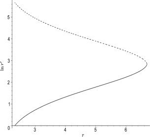
The maximum value of occurs at the cosmological radius and, thereafter, continues to increase as decreases again. The geometrical interpretation of this result is illustrated in Fig. 4, with one spatial dimension suppressed.

In essence, as increases, one is following a great circle on the surface of a sphere, starting at the original point mass and ending at an image mass at the antipodal point of the universe.
We note that there is an interesting relationship between any two values that correspond to the same value of . If two such values are and , then
| (47) |
Since the right-hand side is a function only of , then at any given cosmic time the values and are reciprocally related. This behaviour also occurs in the case of a pure closed FRW model, as discussed in Lasenby et al. (1998).
So far, we have left undetermined, but one can in fact obtain an expression for by combining the standard partial derivative reciprocity relation
| (48) |
with the expression (43) for , which gives
| (49) |
Finding the derivatives of from (45) and equating this result with our integral expression (39) for then yields
| (50) |
Although we do not have an explicit expression for , we have shown that there is an operational method for determining it (i.e. where becomes singular when numerically propagating it inwards from the cosmological radius). If we know and at each time slice (see below for the latter), we can evaluate the above integral for . The only remaining ambiguity is an arbitrary additive constant, which corresponds to an arbitrary multiplicative constant in the definition of in terms of , i.e. it is not possible to identify a unique overall scale for , which seems reasonable.
We note that our solution involving an ‘image mass’ at the antipodal point of the universe ties in with the scenario recently investigated by Uzan, Ellis & Larena (2011), who also considered a closed universe with masses embedded symmetrically at opposite poles. They showed a static solution was not possible for this case, which fits in well with the fact that here we have an explicit exact solution for the masses embedded in an expanding universe. The exact nature of the correspondence with their work will be the subject of future investigation, however.
2.3.3 Cosmological evolution
When considered as a function of the new radial coordinate , the radial derivative of is given by
| (51) |
In Section 2.3.1, we showed that is finite at the cosmological radius , whereas (42) shows that there. Thus, we conclude that at this point. From (22), this corresponds physically to the gradient of the fluid pressure vanishing at the cosmological radius. It appears, therefore, that the fluid pressure at this point can be any function of alone; once this is specified, one has sufficient information to solve jointly for and . This seems plausible physically, since we have not specified an equation of state relation between and , and so need instead to specify a boundary condition on at the cosmological radius.
Let us consider the specific case in which we impose as our boundary condition at , given by (35), for all . Remembering that is given by (36) and using (22) and the standard cosmological field equations, one can then show that
| (52) |
We can therefore, in principle, obtain the expansion history by solving this second-order differential equation. In the limit , an approximate first-integral of the equation is given by
| (53) |
where is a constant. Substituting this result into the expression for given in (57), the corresponding expression for the fluid density is given by
| (54) |
This shows that the presence of the point mass means that does not quite dilute by the usual factor.
3 Comparison with McVittie’s metric
At the same time that McVittie derived his metric (5) for a mass particle in a spatially-flat expanding universe, he also attempted to extend his result to apply to a universe with arbitrary spatial curvature (McVittie, 1933, 1956):
| (55) |
We now compare our metrics for , and with this result.
3.1 Spatially-flat universe
We first note that our metric (23) behaves similarly to McVittie’s metric (5) in the appropriate limits, as it should. In fact, we now show that our metric and McVittie’s are related by a coordinate transformation, despite the fact that they were derived in very different ways. We deduce this relationship by comparing specific physical quantities. Assuming a perfect fluid energy-momentum tensor, precise forms for the density and pressure can be derived from the metrics (Carrera & Giulini, 2010a, b), without assuming the relationship (22), which may not hold for McVittie’s metrics. The resulting quantities are given in Table 2, assuming for simplicity that (although our conclusions still hold in the case).
| McVittie | This work | |
|---|---|---|
It is found that the background densities already match in both models and correspond to the density obtained from the FRW metric; this is not suprising since we are still working within an FRW background. We can use the different forms for the pressure to define a coordinate transformation:
| (56) |
It is easily shown that our metric is equal to McVittie’s metric under this transformation. The transformation actually converts our ‘physical’ radial coordinate to its comoving and isotropic analogue in a single step. Hence our metric describes the same spacetime as McVittie’s metric, with the bonus that its interpretation is more transparent in our non-comoving coordinates. Note that the limit corresponds to , leading back to the FRW pressure in both cases, as expected. The limit on the other hand, which also corresponds to , is not well-defined. As pointed out by Nolan (1998, 1999a, 1999b), and more recently Faraoni & Jacques (2007), it is clear that there is a spacelike singularity in McVittie’s metric at , corresponding to a diverging pressure. The interpretation of this singularity has been under debate for some time, but we now see that it corresponds simply to the physical singularity at in our coordinate system. This in turn coincides with the location of the event horizon from which the background fluid is unable to escape, as discussed in Section 2.1. Thus McVittie’s metric can only be valid for .
This transformation to ‘physical’ coordinates has also previously been pointed out by Nolan (1998, 1999a) and other authors (Arakida, 2009; Bolen, Bombelli & Puzio, 2001; Faraoni & Jacques, 2007). They have also highlighted the ‘accident’ by which McVittie initially derived his metric, which in its original form does not describe a central mass. The mass is located at in our setup, but this does not correspond to the radial coordinate . Instead the point mass is located at , which seems rather unnatural. McVittie’s accident led to problems in the cases of spatially curved cosmologies, as we shall see shortly.
Nolan (1999a) used the transformation (56) to allow for a more intuitive analysis of the global properties of McVittie’s metric. In particular, Nolan identified the function in (12) as the Misner–Sharp energy of the spacetime (Misner & Sharp, 1964). This is a measure of the ‘total energy’ of each fluid sphere in terms of the work done on it by the surrounding fluid. We note that this was the starting point in our derivation of the metric (23), as opposed to an emergent feature. It therefore clarifies a point that has been under debate for a long time; McVittie’s metric does indeed describe a point-mass in an otherwise spatially-flat FRW universe (see also Kaloper, Kleban & Martin (2010) and Lake & Abdelqader (2011)).
3.2 Spatially-curved universe
We have already shown that an advantage of our approach is that we have a natural way of generalising to the case of a curved cosmology. For , our model still incorporates an FRW background so we would again expect our form for not to deviate from the standard FRW result; in particular, it should be a function of only. Indeed, using the general metric (8) with and given in Table 1, we find (again assuming for simplicity)
| (57) |
where the series solutions for for the cases and are given in (28) and (40), respectively.
For McVittie’s metric (55), however, we find the peculiar feature that the background density does depend on the radial coordinate :
| (58) |
where (Nolan, 1998). This is odd since the only apparent difference between this model and the spatially-flat case is the spacetime curvature. McVittie’s metrics hence cannot describe a mass particle embedded in a background with homogeneous density. Indeed the density and pressure (58) do not even asymptotically tend to the FRW solutions.
Our metrics, which are derived by explicitly assuming a model of a point mass embedded in a homogeneous background, are therefore inherently different to McVittie’s solutions. Nolan (1998) has used a model similar to ours to obtain a metric in the case that is expressed in terms of an elliptic function, but we have not yet found a coordinate transformation that equates this with our solution. A full comparison will be the subject of future research.
4 Geodesic motion in the spatially-flat metric
The motion of a test particle moving under gravity around a central point mass in a static spacetime has been very well studied. In simple terms, we would expect the incorporation of an expanding background to provide an additional ‘force’ that alters the trajectory of the test particle. We investigate this possibility by first calculating the geodesic equations for our metric, using the usual ‘Lagrangian’ technique. We restrict our attention to the case, since observations indicate the universe to be very close to spatially flat (Larson et al., 2011).
Working in the equatorial plane , the ‘Lagrangian’ corresponding to our flat metric (23) is
where dots denote differentiation with respect to the proper time of the test particle. The three remaining geodesic equations are obtained from the Euler-Lagrange equations for , and . For stationary, spherically-symmetric metrics, such as the Schwarzschild metric, one can immediately obtain the first integrals of the and geodesic equations. Moreover, it is usual to replace the geodesic equation by its first integral (for timelike geodesics). These three equations can then be easily combined to obtain an ‘energy equation’ in terms of , and constants of the motion only. By differentiating this equation, a simple expression for can be obtained, if desired. This procedure is followed for the Schwarzschild de Sitter metric by Balaguera-Antolínez, Böhmer & Nowakowski (2006). Our metric, however, is a function of both and , and therefore this standard approach does not prove useful in finding and the procedure must be modified.
In our case, the geodesic equation is not replaced since it contains an term. This is of particular interest to us in determining the nature of the gravitational ‘forces’ acting on the particle. The geodesic equation is , where is the specific angular momentum of the test particle. Substituting this into the equation and rearranging gives
| (59) |
The term can be eliminated completely using the -equation, so that (59) now becomes
| (60) |
Note that the terms above, when combined, differ very slightly from that derived in Carrera & Giulini (2010b); we believe the latter to be in error. We now use the condition to eliminate the terms. After some algebraic manipulation this finally leads to a relatively simple exact expression for , namely
| (61) |
4.1 Newtonian limit and forces
It is of interest to consider special cases of (61). First we consider the weak field approximation by assuming and expanding to leading order in small quantities. We also take the low-velocity limit , . In this Newtonian limit, we find
| (62) |
where is the deceleration parameter. This result can also be obtained directly from our flat metric (23) in its Newtonian limit (Nesseris & Perivolaropoulos, 2004):
| (63) |
Note that this incorporates the usual low velocity approximation, but the weak field condition used is simply . Incorporating the condition as well simply leads to the flat Minkowski metric, which does not effectively describe the physical system in which we are interested.
We may interpret (62) as the physical acceleration of the test particle in the Newtonian limit, and hence the gravitational force per unit mass acting upon it. Aside from the ‘centrifugal’ term depending on the specific angular momentum , the terms in (62) correspond to the standard inwards force due to the central mass and a cosmological force proportional to that is directed outwards (inwards) when the expansion of the universe is accelerating (decelerating).
An interesting feature of the cosmological force is that its direction (and magnitude) depends on whether the universe is accelerating or decelerating (as determined by the sign of ). This was pointed out previously by Davis, Lineweaver & Webb (2003), and highlights the common misconception of there being some force or drag associated simply with the expansion of space; instead the force is better associated with the acceleration/deceleration of the expansion. In particular, we note that if the universe is decelerating, the cosmological force is directed inwards and the test particle inevitably moves towards the central mass , falls through its position and joins onto the Hubble flow on the other side. This does not, however, argue against the idea of the expansion of space.
Since the current deceleration parameter of the universe is measured to be approximately (Larson et al., 2011), we see that the present-day cosmological force is directed outwards, as one might have naively expected intuitively. However, since the expansion history of the current concordance model of cosmology changes from a decelerating phase to an accelerating phase at a relatively recent cosmic time, the cosmological force must reverse direction at this epoch. A realistic scale factor corresponding to the standard spatially-flat concordance model is (Hobson, Efstathiou & Lasenby, 2006):
where (Larson et al., 2011) is the current fraction of the critical density of the universe in the form of dark energy. Using this expression, in Fig. 5 we plot the ratio of the cosmological force relative to its present-day value, as a function of redshift . As anticipated, we see that the cosmological force reverses direction; it is an inwards force for redshifts larger than about . Moreover, the magnitude of the force relative to its current value increases by a factor of by about and by a factor of nearly by ; it continues to grow with redshift quickly thereafter.

The cosmological force appears to have been correctly taken into account in cosmological simulation codes. For example, in Springel, Yoshida & White (2001) and Springel (2005), dark matter and stars are modelled as self-gravitating collisionless fluids following the collisionless Boltzmann equation, and this term appears in the equation of motion of the particles. For a single central mass , the equation of motion of a test particle is taken as
| (64) |
where represents comoving coordinates. Converting to ‘physical’ coordinates via recovers the result (62) with .
We perform a full exploration of the astrophysical consequences of the geodesic equation (62) in our companion paper NLH2. We also note that Price (2005) has used a very similar geodesic equation to analyse the motion of an electron orbiting a central nucleus, with a slight modification to account for the dominant electrostatic force in that problem. An extension of this work is also presented in NLH2.
4.2 Particle released from rest
It is, of course, of interest to calculate the ‘force’ experienced by the particle in the fully general-relativistic case. This is discussed in detail in the next section, but as a prelude let us return briefly to (61) and consider a particle released from rest, for which . Thus, instantaneously, one has
| (65) |
One should bear in mind at this point, however, that the ‘physical’ coordinate is not a proper radial distance. Hence one cannot simply interpret (65) as the instantaneous force on a particle released from rest, or equivalently the negative of the force required to keep a test particle at rest relative to the central point mass. The proper expression for this force is derived in the next section.
5 Frames and forces
We now derive a fully general-relativistic invariant expression, valid for any spherically-symmetric system, for the radial force required to hold a test particle at rest relative to the central point mass. We first point out that the relationship between the ‘physical’ coordinate and proper radial distance to the point mass is defined through . It is therefore only in the spatially-flat case, for which is independent of , that or are equivalent conditions. In general, one must thus choose which condition defines ‘at rest’. Here we will adopt the condition , which corresponds physically to keeping the test particle on the surface of a sphere with proper area . In practice, it would probably be easier for an astronaut (i.e. test particle) to make a local measurement to determine the proper area of the sphere on which he is located, rather than to determine his proper distance to the point mass, particularly in the presence of horizons. With this proviso, our derivation is valid for arbitrary tetrad components , and (but we assume the Newtonian gauge ).
In general, the invariant force (per unit mass) acting on a particle is equal simply to its proper acceleration, i.e. the acceleration of the particle as measured in its instantaneous rest frame. We must therefore find an expression for the proper acceleration of a particle held at rest relative to the central point mass. This may be calculated directly in the coordinate basis, but it is more instructive for our purposes, and simpler, to perform the calculation in the tetrad frame.
5.1 Tetrad frames and observers
The tetrad frame defines a family of ideal observers, such that the integral curves of the timelike unit vector field are the worldlines of these observers, and at each event along a given worldline, the three spacelike unit vector fields specify the spatial triad carried by the observer. The triad may be thought of as defining the spatial coordinate axes of a local laboratory frame, which is valid very near the observer’s worldline. In general, the worldlines of these observers need not be timelike geodesics, and hence the observers may be accelerating.
Let us first consider the four-velocity and proper acceleration of the observer defined by our tetrad frame (7). The four-velocity of the observer is simply , so that, by construction, the components of the four-velocity in the tetrad frame are . Since , the four-velocity may be written in terms of the tetrad components and the coordinate basis vectors as . Thus, the components of the observer’s four-velocity in the coordinate basis are simply , where dots denote differentiation with respect to the observer’s proper time. Hence, for all our previously derived metrics, we see from Table 1 that . Since the comoving radial coordinate is defined through , we deduce that . Hence the observer is not comoving with the Hubble flow. Instead, since is negative, the observer’s comoving radial coordinate is decreasing.
This behaviour is due to the presence of the central point mass, which results in our observer not moving geodesically (except as ). This is easily seen by calculating the proper acceleration of our observer, which is given by , where is the four-acceleration of the observer.
It is straightforward to show that, for a body moving with general four-velocity , the four-acceleration is given in terms of the coordinate basis and the tetrad basis respectively by
| (66) |
where are the connection coefficients corresponding to the metric (8) and
| (67) |
are known as Ricci’s coefficients of rotation or the spin-connection. It has been shown by, for example, Kibble (1961) that these can be written in terms of the tetrad components as
| (68) |
It follows that is anti-symmetric in the first two indices, and is anti-symmetric in the last two indices. For general radial motion , in which case the components of the four-acceleration in the tetrad frame reduce to
| (69) |
and . It follows that for general radial motion only () and () need to be computed. Using (68), the definitions of the tetrads and their inverses (7) and the relations given in equation (10), one can show that
| (70) |
This highlights that the functions and defined earlier are in fact components of the spin-connection; indeed this is how Lasenby et al. (1998) originally defined them, but using geometric algebra. Hence the components of the four-acceleration in the tetrad frame for general radial motion are
| (71) |
If we now specialise to the case where , the four-velocity of our observer, then , and so . Thus the proper acceleration of our observer is , which coincides with our earlier identification of as a radial acceleration. Equivalently, the invariant force per unit rest mass (provided, for example, by a rocket engine) required to keep the observer in this state of motion has magnitude in the outwards radial direction.
5.2 Radially-moving test particle
Let us now consider a particle in general radial motion such that its four-velocity components in the tetrad frame are
| (72) |
where is the particle’s rapidity in that frame and is the particle’s proper time. Using the tetrad definitions (7) one can show that these components are related to those in the coordinate basis by
| (73) |
Substituting the coefficients (72) into the equations in (71), we find that the components of the particle’s four-acceleration in the tetrad frame are given by
| (74) |
Thus, the particle’s proper acceleration , and hence the invariant force per unit rest mass required to maintain the particle in this state of motion, is
| (75) |
5.3 Force required to keep test particle at rest
We now consider the special case of a particle at rest relative to the central point mass. In this case, and from (73) it is found that . Moreover, since the magnitude of the four-velocity must be unity, we deduce that . Hence, the four-velocity (72) may be written
| (78) |
Using these expressions for and in (75), the force per unit rest mass required to keep the test particle at rest is found to be
| (79) |
For general radial motion, , but in this case and from (73) and (78) we find . We thus obtain
| (80) |
Hence, the required force is determined by the tetrad components themselves and also some of their derivatives with respect to and (the latter through the functions and ).
It is of interest to compare our expression for in (79) with the expression (77) for in the special case of a particle released from rest, for which and . In this case, using (78), we find that, instantaneously,
| (81) |
Thus, we see that the force (per unit rest mass) in (79) required to keep a test particle at rest is related to the instantaneous value of for a particle released from rest by
| (82) |
The force expression (80) in this general form can be applied to any spherically-symmetric system for which the required quantities can be computed. Below, we will obtain the expressions for in each of our newly-derived metrics. Before we consider each metric separately, however, it is worth noting that the force (80) becomes singular at any point where . In the case of our newly derived metrics, we see from Table 1 that this corresponds to where
| (83) |
which is valid for and . Introducing the curvature density parameter , where is the total density parameter, the above condition becomes
| (84) |
Comparing this condition with (34), we see that one has simply replaced by . Consequently, provided , (84) has three real roots, one of which lies at negative and the remaining two lie at and given by (35), but with replaced by . In particular, the force becomes infinite outside the Schwarzschild radius and inside the ‘scaled’ Hubble radius .
5.3.1 Spatially-flat universe
The functions defining the metric for a point mass embedded in a spatially-flat universe are given in Table 1. To calculate , we must also evaluate and , which are easily shown to be
| (85) |
Thus the outward force required to keep a test particle at rest relative to the central point mass is
| (86) |
Comparing (86) with the expression (65) giving the instantaneous value of for a particle released from rest in this spacetime, we see that they indeed obey the relationship (82). Assuming , expanding (86) in small quantities one finds that the zeroth order term is simply , consistent with Newtonian gravity. We are interested in where the cosmological expansion parameter enters into the force expression, and we find that it does so at first order in small quantities. Keeping the leading terms, one obtains
| (87) |
which is consistent with the corresponding equation of motion (62) in the Newtonian limit for a particle moving radially under gravity. Finally, for comparison against the equivalent open and closed universe results, note that keeping all terms up to second order in small quantities leads to the expression
| (88) |
5.3.2 Open universe
The functions defining the metric are listed in Table 1, and it can be shown that and are given by
| (89) |
Thus the expression for the required outward force is
| (90) |
In the limit , this expression reduces to the force (86) in the spatially-flat case, as might be expected.
Assuming that , expanding (90) in small quantities and keeping only the leading terms at first order, the force is found to be given by equation (87). Thus in this limit the force in an open universe is indistiguishable from that in a spatially-flat universe. The differences between the two become visible only when expanding up to second order in small quantities:
| (91) |
The only difference between this expression and the corresponding spatially-flat result (88) is the extra negative contribution proportional to . This can be interpreted as an ‘anti-gravitational’ force experienced by the test particle due to a virtual ‘image’ mass dragged out to the curvature scale of the universe. Since this term is negligible compared to the term, and hence the force is not significantly altered relatively to the spatially-flat case.
5.3.3 Closed universe
The functions defining the closed universe () metric are listed in Table 1. In this case,
| (92) |
Thus the expression for the required outward force is
| (93) |
In the limit , this expression also reduces to the force (86) in the spatially-flat case.
Assuming that , expanding (93) in small quantities and keeping the leading terms up to first order, the force is once again found to be given by equation (87). In this limit the force in a closed universe is thus indistiguishable from that in a spatially-flat or open universe. Any differences again only become visible when expanding up to second order in small quantities:
| (94) |
Thus we see that the only difference between this force and the corresponding result (91) for an open universe is the sign of the extra contribution proportional to . In a closed universe, this contribution to the force by the ‘image’ mass, which in this case can be viewed as a real object, is of the same sign as that due to the original mass. Once again, however, since this term is negligible compared to the term, and hence the force is not significantly altered relative to the spatially-flat case.
6 Discussion and conclusions
In this paper, we have presented a tetrad-based method for solving Einstein’s field equations in general relativity for spherically-symmetric systems. Our method is essentially a translation of the method originally presented by Lasenby et al. (1998) in the language of geometric algebra.
We use this technique to derive the metrics describing a point mass embedded in an homogeneous and isotropic expanding fluid, for a spatially-flat, open and closed universe, respectively. In the closed universe case, the lack of the notion of spatial infinity means that considerable care is required to determine the appropriate boundary conditions on the solution. We find that in the spatially-flat case, our metric is related by a coordinate transformation to the corresponding metric derived by McVittie (1933). Nonetheless, our use of ‘physical’ coordinates greatly facilitates the physical interpretaion of the solution. For the open and closed universes, however, our metrics differ from the corresponding McVittie metrics, which we believe to be incorrect.
We derive the geodesic equation for the motion of a test particle under gravity in our spatially-flat metric. For radial motion in the Newtonian limit, we find that the gravitational force on a test particle consists of the standard inwards force due to the central mass and a cosmological force proportional to that is directed outwards (inwards) when the expansion of the universe is accelerating (decelerating). For the standard CDM concordance cosmology, the cosmological force thus reverses direction at about , when the expansion of the universe makes a transition from a decelerating to an accelerating phase. It is expected that this phenomenon has a significant impact on the growth and evolution of structure, particularly around ; a detailed investigation of this is a subject for further study. Nonetheless, we believe this effect is implicitly included in existing numerical simulation codes. In our companion paper NLH2, we will show how the cosmological force leads to a maximum size for a bound object such as a galaxy or cluster, and explore the stability of bound orbits around the central mass.
We also used our tetrad-based approach to derive an invariant fully general-relativistic expression, valid for arbitrary spherically-symmetric systems, for the force required to keep a test particle at rest relative to the central mass. We apply this result to our derived metrics in the spatially-flat, open and closed cases. To first order in small quantities the force in all three cases is the same, but differences become visible when considering the second order terms. Interestingly, we find that the force in an open universe has an additional component that may be interpreted as a gravitationally repulsive term due to an ‘image’ mass dragged out to the curvature scale of the universe. A similar term, but with the opposite sign, is present in the force in a closed universe, and results from an image mass at the antipodal point of the universe. In both cases, however, the additional components are neglible at distances from the original central mass that are small compared with the curvature scale, and so in practical terms the force in a spatially-curved universe is not significantly different from that in the spatially-flat case.
It must be pointed out that our assumption that the background fluid density is spatially uniform may be questionable, since the point mass breaks homogeneity. The correct treatment of the background may require also to depend on the radial coordinate , which would significantly complicate the equations and would probably not yield analytical solutions. It is interesting that McVittie’s solutions do in fact yield background densities dependent on both and . Nonetheless, since the point mass in our model does not occupy any space in the background, and also because we have ultimately been interested in , assuming is a good approximation. Note that we will improve our model by accounting for the finite size of the central object in a subsequent paper. We will consider only spatially homogenous objects for simplicity, but we leave the consideration of more general radial density profiles for future research. We also note that our approach may be extended to systems with accretion onto the central mass by the replacement of in equation (12); a full analysis of this will also be presented in a future publication.
Acknowledgements
RN is supported by a Research Studentship from the Science and Technology Facilities Council (STFC).
References
- Arakida (2009) Arakida H., 2009, New Astronomy, 14, 264
- Balaguera-Antolínez, Böhmer & Nowakowski (2006) Balaguera-Antolínez A., Böhmer G.C., Nowakowski M., 2006, Class. Quant. Grav., 23, 485
- Binney & Tremaine (2008) Binney J., Tremaine S., 2008, Galactic Dynamics, 2nd Ed., Princeton University Press
- Bolen, Bombelli & Puzio (2001) Bolen B., Bombelli L., Puzio R., 2001, Class. Quant. Grav., 18, 1173
- Carrera & Giulini (2010a) Carrera M., Giulini D., 2010, Phys. Rev. D, 81,043521
- Carrera & Giulini (2010b) Carrera M., Giulini D., 2010, Rev. Mod. Phys., 82, 169
- Carroll (2003) Carroll S.M., 2003, Spacetime and Geometry, Addison Wesley, New York
- Davis, Lineweaver & Webb (2003) Davis T.M., Lineweaver C.H., Webb J.K., 2003, American Journal of Physics, 71, 358
- Faraoni & Jacques (2007) Faraoni V., Jacques A., 2007, Phys. Rev. D, 76, 063510
- Hobson, Efstathiou & Lasenby (2006) Hobson M.P., Efstathiou G., Lasenby A.N., 2006. General Relativity, Cambridge University Press, New York
- Kaloper, Kleban & Martin (2010) Kaloper N., Kleban K., Martin D., 2010, Phys. Rev. D, 81, 104044
- Kibble (1961) Kibble T.W.B., 1961, J. Math. Phys., 2, 212
- Lake & Abdelqader (2011) Lake K., Abdelqader M., 2011, Phys. Rev. D, 84, 044045
- Larson et al. (2011) Larson D. et al., 2011, ApJSS, 192, 16
- Lasenby et al. (1998) Lasenby A., Doran C., Gull S., 1998, Phil. Trans. R. Soc. Lond. A, 356, 487
- Lynden-Bell (1967) Lynden-Bell D., 1967, MNRAS, 136, 101
- McVittie (1933) McVittie G.C., 1933, MNRAS, 93, 325
- McVittie (1956) McVittie G.C., 1956, The Int. Astrophys. Ser., General Relativity and Cosmology, Chapman & Hall, London
- Misner & Sharp (1964) Misner C.W., Sharp D.H., 1964, Phys. Rev., 136, B571
- Nandra, Lasenby & Hobson (2011) Nandra R., Lasenby A.N., Hobson M.P., 2012, MNRAS (NLH2), 422, 2945
- Nesseris & Perivolaropoulos (2004) Nesseris S., Perivolaropoulos L., 2004, Phys. Rev. D, 70, 123529
- Nolan (1998) Nolan B.C., 1998, Phys. Rev. D, 58, 064006
- Nolan (1999a) Nolan B.C., 1999, Class. Quant. Grav., 16, 1227
- Nolan (1999b) Nolan B.C., 1999, Class. Quant. Grav., 16, 3183
- Price (2005) Price R.H., 2005, arXiv:gr-qc/0508052v2
- Springel, Yoshida & White (2001) Springel V., Yoshida N., White S.D.M., 2001, New Astronomy, 6, 79
- Springel (2005) Springel V., 2005, MNRAS, 364, 1105
- Uzan, Ellis & Larena (2011) Uzan J.-P., Ellis G.F.R., Larena J., 2011, Gen. Rel. Grav., 43, 191