Higgs Inflation in Horava-Lifshitz Gravity

Abstract

We study the possibility of standard model Higgs boson acting as an inflaton field in the framework of Horava-Lifshitz Gravity. Under this framework, we showed that it is possible for the Higgs field to produce right amount of inflation and generate scale invariant power spectrum with the correct experimental value. Thanks to the foliation preserving diffeomorphism and anisotropic space-time scaling, it essentially helps us to construct this model without the pre-existing inconsistency coming from cosmological and particle physics constraints. We do not need to introduce any non-minimal or higher derivative coupling term in an arbitrary basis either.

Introduction. It has been widely accepted that our universe has experienced an exponential expansion in the very early stage of its evolution. Thanks to this exponential expansion, it explains the flatness and homogeneity of our universe. It also helps to get rid of heavy particles such as monopoles which would otherwise alter the present state of evolution of our universe. This exponential expansion is called Inflation Guth:1980zm ; Albrecht:1982wi ; Linde:1983gd . Most interestingly, inflation also helps the quantum fluctuations to evolve into a classical curvature perturbation which eventually sources the seed of structure formation in our universe. By choosing a particular model of inflation, the primordial power spectrum for the curvature perturbation can be made scale-invariant which fits very well with the latest WMAP data Larson:2010gs . Moreover, all the other known cosmological observations also support the inflation in the early universe.

Constructing a model of inflation has been the subject of interest for the last several decades. The simplest and phenomenologically most successful model of inflation so far is a model of a single scalar field called inflaton which drives the exponential expansion. One of the fundamental issues with the standard inflationary model is the origin of the scalar field. As we know standard model of particle physics which is most successful, contains a natural scalar field called Higgs. Although Higgs field has not been observed yet, it would be natural and also economical if one can identify this Higgs as an inflaton field. However, because of the strong self-coupling which is constrained by the particle physics, it has been ignored in the past in the inflationary model building. The reason can be seen from a straightforward estimation of the power spectrum for a minimally coupled Higgs field with the following action,

$${\cal S}_{H}=\int d^{4}x\sqrt{-g}[\kappa^{2}R-\frac{1}{2}D_{\mu}{\bf H}^{\dagger}D^{\mu}{\bf H}-\frac{\lambda_{H}}{4}({\bf H}^{\dagger}{\bf H}-v^{2})^{2}]~{},$$ (1)

where $\kappa^{2}\equiv 1/(16\pi G)$, $R$ is the Ricci scalar, $\bf{H}$ is Higgs boson doublet, $D_{\mu}$ is the covariant derivative with respect to $SU(2)\times U(1)$ gauge group, $\lambda_{H}$ is the self-coupling coefficient and $v$ is the vacuum expectation value (VEV) of the Higgs. Hereafter, we adopt the metric to be

$$ds^{2}=dt^{2}-a^{2}(t)dx^{2}~{}.$$ (2)

At the energy scale of inflation we can ignore the VEV of the Higgs field. The action therefore turns out to be:

$${\cal S}_{H}=\int d^{4}x\sqrt{-g}[\kappa^{2}R-\frac{1}{2}\partial_{\mu}\phi\partial^{\mu}\phi-\frac{\lambda_{H}}{4}\phi^{4}]~{},$$ (3)

where we consider a real scalar field $\phi$ in place of ${\bf H}$ for simplicity. The equations of motion for the metric and $\phi$ are:

$$H^{2}=\frac{8\pi G}{3}(\frac{1}{2}\dot{\phi}^{2}+\frac{\lambda_{H}}{4}\phi^{4})~{},~{}~{}~{}\ddot{\phi}+3H\dot{\phi}+\lambda_{H}\phi^{3}=0~{},$$ (4)

where $H$ denotes the Hubble parameter and ${\dot{H}}=dH/dt$. In order to get sufficient efolding, we impose a “slow-roll” condition

$$\epsilon\equiv-\frac{\dot{H}}{H^{2}}\simeq\frac{\kappa^{2}}{\phi^{2}}\ll 1~{},$$ (5)

which essentially sets $\phi\gg 1$ in Planck unit. Now following Ref. Stewart:1993bc , the primordial power spectrum of the curvature perturbation turns out to be:

$${\cal P}_{\zeta}\equiv\frac{k^{3}}{2\pi}|\zeta|^{2}\sim\frac{H^{4}}{2\pi\dot{\phi}}\sim\frac{H^{2}}{\epsilon}\sim\frac{V^{3}}{V_{\phi}^{2}}\sim\lambda_{H}\phi^{6}~{}.$$ (6)

If we take $\phi>1$, the observed power spectrum ${\cal P}_{\zeta}\sim 10^{-9}$ sets the limit on $\lambda_{H}$ to be $\leq 10^{-9}$. This is in direct conflict with the standard model prediction of Higgs coupling $0.11<\lambda_{H}\lesssim 0.27$ Amsler:2008zzb . This severe constraint makes it difficult to construct a minimally coupled Higgs inflationary model.

In order to get rid of this inconsistency, only recently people have come up with a non-trivial modification of Higgs action with the gravity CervantesCota:1995tz ; Bezrukov:2007ep ; Germani:2010gm ; Kamada:2010qe . The simplest non-minimal coupling term that has been introduced Bezrukov:2007ep is $\xi R\phi^{2}$ where $\xi$ is the coupling constant. In this model considering the slow-roll parameter $\epsilon\simeq\xi^{-2}\phi^{-4}$, the expression for the efolding number becomes ${\cal N}\simeq\xi\phi^{2}$. Thus required amount of ${\cal N}$ gives $\phi\sim 10/\sqrt{\xi}$. Considering this constraint on $\phi$ and $0.11<\lambda_{H}\lesssim 0.27$, one can easily produce the experimental value of the power spectrum ${\cal P}_{\zeta}\sim\lambda_{H}\phi^{4}\sim\lambda_{H}\xi^{-2}\sim{\cal O}(10^{-9})$ by choosing the new parameter $\xi>10^{4}$. However, later it has been pointed out that, this scenario is plagued with the unitarity problem. More specifically, at the quantum level, this non-minimal coupling term $\xi\delta\phi^{2}\partial^{2}\gamma$ ($\gamma\equiv Tr(\gamma_{\mu\nu})$), where $\delta\phi=\phi-\phi_{0}$ and $\gamma_{\mu\nu}=g_{\mu\nu}-\eta_{\mu\nu}$ are the quantum fluctuation around the background Burgess:2009ea , will violate the unitarity of S-matrix at an energy scale $\Lambda\simeq\xi^{-1}$. This should be considered as a cut-off for the effective theory. This scale scale turns out to be much below the typical fluctuation of the Higgs field during inflation as discussed above Lerner:2009na .

To circumvent the above mentioned problem, the authors in Germani:2010gm introduced an alternative kinetic coupling of the Higgs field with gravity of the form $G^{\mu\nu}\partial_{\mu}\phi\partial_{\nu}\phi$, where $G^{\mu\nu}$ is the Einstein tensor. This new non-minimal coupling term also gives rise to a unitarity bound $\Lambda(H)\simeq(2H^{2}/\kappa)^{1/3}$ but the claim is that this bound is well above the gravitational energy scale during inflation. However, soon after this, a careful analysis has been done in Atkins:2010yg and showed that unitariry is actually violated in this model as well. In an another attempt authors of Kamada:2010qe have introduced a non-trivial higher derivative kinetic term $G((\partial\phi)^{2},\phi)\Box\phi$ in addition to the usual Higgs Lagrangian. This construction is inspired by the recently proposed theory called Galileon theory Nicolis:2008in . The important property of this new terms is that it does not lead to an extra degrees of freedom (ghost) because the equation of motion for the Higgs field is still second order in derivative. This new term modifies the dispersion relation of the scalar field and helps to produce the sufficient number of efolding as well as required amplitude of power spectrum. However, more detail study needs to be done regarding the unitarity problems of this kind of model.

In this Letter, we propose a new scenario where Higgs inflation can be realized in the framework of Horava-Lifshitz (HL) gravity Horava:2009uw . HL theory of gravity is known to be invariant under a foliation perserving diffeomorphism

$$\tilde{x}^{i}=\tilde{x}^{i}(x^{j},t)~{},~{}~{}~{}\tilde{t}=\tilde{t}(t)~{}.$$ (7)

Interestingly, the theory can be made power counting renormalizable in four dimension if one introduces an anisotropic scaling transformation of space and time like

$$\overrightarrow{x}\rightarrow b\overrightarrow{x}~{},~{}~{}~{}t\rightarrow b^{3}t.$$ (8)

Moreover, it is also argued that in the low energy limit, theory flows to the standard General Relativity (GR) where the full diffeomorphism invariance is recovered as an emerging symmetry. All these interesting properties trigger a spate of research works in the diverse directions for the last few years, see the current status of HL theory from the reviews Mukohyama:2010xz . Although the original version of Horava gravity may be plagued by the extra unwanted degrees of freedom Charmousis:2009tc , later on different extensions have been proposed in order to cure this Blas:2009qj ; Horava:2010zj . In this letter we will adopt the original version of the Horava gravity to construct the Higgs inflationary model, while leaving concerns over the other versions of Horava gravity for our future study.

Higgs Inflation in HL Gravity. With the symmetry under consideration, it is customary to consider the $3+1$ decomposition of the space-time metric:

$$ds^{2}=N^{2}dt-h_{ij}(dx^{i}+N^{i}dt)(dx^{j}+N^{j}dt)~{},$$ (9)

where $N(t,\overrightarrow{x})$, $N_{i}(t,\overrightarrow{x})$ and $h_{ij}$ are the lapse function and the shift vector and the spatial metric respectively. The most general HL action without the condition of detailed balance will be of the form :

$$\mathcal{S}=\kappa^{2}\int dtd^{3}xN\sqrt{g}(\mathcal{L}_{K}-\mathcal{L}_{V}+\kappa^{-2}\mathcal{L}_{M})~{},$$ (10)

where

$$\mathcal{L}_{K} = K_{ij}K^{ij}-\lambda K^{2}~{},$$ (11)

$$\mathcal{L}_{V} = 2\Lambda-R+\kappa^{-2}(g_{2}R^{2}+g_{3}R_{ij}R^{ij})$$ (12)

$$+ \kappa^{-4}(g_{4}R^{3}+g_{5}RR_{ij}R^{ij}+g_{6}R_{j}^{i}R_{k}^{j}R_{i}^{k})$$

$$+ \kappa^{-4}(g_{7}R\nabla^{2}R+g_{8}(\nabla_{i}R_{jk})(\nabla^{i}R^{jk}))~{},$$

$$\mathcal{L}_{M} = \frac{1}{2N^{2}}(\dot{\phi}-N^{i}\nabla_{i}\phi)^{2}-\mathcal{V}(\phi,g_{ij})~{},$$ (13)

here $K_{ij}\equiv(\dot{h}_{ij}-\nabla_{i}N_{j}-\nabla_{j}N_{i})/(2N)$ is the extrinsic curvature, and $\lambda$ is a free parameter. In IR region, $\lambda$ flows to unity to recover GR. The potential term reads:

$$\mathcal{V}(\phi,g_{ij}) = V_{0}(\phi)+V_{1}(\phi)(\nabla\phi)^{2}+V_{2}(\phi)(\Delta\phi)^{2}$$ (14)

$$+ V_{3}(\phi)(\Delta\phi)^{3}+V_{4}(\phi)(\Delta^{2}\phi)$$

$$+ V_{5}(\phi)(\nabla\phi)^{2}(\Delta^{2}\phi)+V_{6}(\phi)(\Delta\phi)(\Delta^{2}\phi)~{}.$$

Note that we consider $\phi$ to be the Higgs field, so the background potential will be $V_{0}(\phi)=\lambda_{H}\phi^{4}/4$. The background equations of motion for the metric (2) and field $\phi$ are:

$$\kappa^{-2}(\frac{1}{2}\dot{\phi}^{2}+V_{0}(\phi))+3H^{2}(1-3\lambda)=0~{},$$ (15)

$$\kappa^{-2}(\frac{1}{2}\dot{\phi}^{2}-V_{0}(\phi))-3H^{2}(1-3\lambda)=2(1-3\lambda)\dot{H}~{}$$ (16)

$$\ddot{\phi}+3H\dot{\phi}+V_{0\phi}=0~{},$$ (17)

where $V_{0\phi}\equiv\partial V_{0}(\phi)/\partial\phi$. We also set cosmological constant $\Lambda=0$. The expression for the slow-roll parameter $\epsilon$ and the number of efoldings ${\cal N}$ will be of the same form as that of the standard GR, namely,

$$\epsilon\equiv-\frac{\dot{H}}{H^{2}}\simeq\kappa^{2}\frac{V_{0\phi}^{2}}{V^{2}}~{},~{}~{}~{}{\cal N}\equiv\int_{t_{i}}^{t_{f}}Hdt\simeq\int_{\phi_{i}}^{\phi_{f}}\frac{V}{V_{0\phi}}d\phi~{}.$$ (18)

As we have discussed, numerically it is easy to find out the solution for slow-roll inflation for sufficiently long period as shown in Fig. 1. We want to emphasize here that in usual Higgs inflation scenario, the Hubble parameter (or scalar potential) is very large because of large $\lambda_{H}$, which eventually leads to a large curvature perturbation compared to the observed power spectrum. Thanks to the foliation preserving diffeomorphism and anisotropic space-time scaling of HL Gravity, in the UV limit it turns out that the evolution of the curvature perturbation depends only on the higher derivative term of the Higgs field and not on its potential . This is the key point that makes the Higgs inflation feasible in the framework of HL gravity.

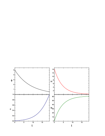
Figure 1: (Colored online.) The evolution of $\phi$, $H$, $\epsilon$ and ${\cal N}$. Horizontal axis is the cosmic time $t$. Parameters and initial values: $\lambda=1.2$, $\lambda_{H}=0.2$, $v=0$, $\phi_{i}=5M_{pl}$, $\dot{\phi}_{i}=0$. The normalization is $M_{pl}=1$. From the figures we can see that at the end of inflation we have approximately $\phi_{f}\simeq 0.54M_{pl}$ and $H_{f}\simeq 0.2M_{pl}$.

Perturbations and Scale-Invariant Power Spectrum. The cosmological perturbation in the HL gravity has been widely studied Gao:2009bx . We expand the scalar field and spatial metric as follows:

$$\phi(t,\overrightarrow{x})=\phi_{0}(t)+Q(t,\overrightarrow{x})~{},~{}~{}~{}h_{ij}=a^{2}(t)e^{2\gamma(t,\overrightarrow{x})}\delta_{ij}~{}.$$ (19)

In the cosmological perturbation theory, it is customary to write down the equations of motion for the perturbation in terms of a gauge invariant variable

$$\zeta=\gamma-\frac{H}{\dot{\phi}_{0}}Q~{},$$ (20)

which is a linear combination of metric and scalar field perturbation. The equation of motion for the gauge invariant perturbation $\zeta$ can be further simplified by defining an another variable $u\equiv a\sqrt{\mathcal{K}}\zeta$ where ${\cal K}$ is given in the appendix. The final equation of motion of our interest would take a very simple form:

$$u^{\prime\prime}+\omega_{u}^{2}u=0~{}.$$ (21)

The modified dispersion relation is

$$\omega_{u}^{2}=\frac{a^{2}\mathcal{M}^{2}}{\mathcal{K}}-(\mathcal{H}+\frac{\mathcal{K}^{\prime}}{2\mathcal{K}})^{2}-(\mathcal{H}+\frac{\mathcal{K}^{\prime}}{2\mathcal{K}})^{\prime}~{},$$ (22)

where “prime” denotes the derivative w.r.t. conformal time $\eta$ with $dt=a(t)d\eta$. The expression for the effective mass $\mathcal{M}$ is also given in the appendix.

It is intuitively obvious that the terms coming from higher spatial derivative will be dominant in the expression for $\omega_{u}$ in UV regime. In Fourier space, the leading order behavior of $\omega_{u}^{2}$ would be $\omega_{u}^{2}\rightarrow a^{2}\kappa^{-4}(1-\lambda)(3g_{8}-8g_{7})\bar{k}^{6}/(1-3\lambda)$, where $\bar{k}\equiv k/a(t)$. $k$ is the wavenumber of fluctuation. The equation of motion therefore becomes

$$u^{\prime\prime}+\frac{a^{2}(1-\lambda)(3g_{8}-8g_{7})\bar{k}^{6}}{\kappa^{4}(1-3\lambda)}u=0~{}.$$ (23)

The solution turns out to be:

$$u\simeq\frac{1}{\sqrt{2\omega_{u}}}\exp\left(i\int\omega_{u}d\eta\right)~{}.$$ (24)

Moreover, amplitude of the fluctuation freezes out at horizon crossing where $\omega_{u}$ is comparable with the Hubble parameter $H$. From the definition of power spectrum (6), we find:

$${\cal P}_{\zeta}=\frac{k^{3}}{2\pi}\big{|}\frac{u}{a\sqrt{\cal K}}\big{|}^{2}\simeq\kappa\left(\frac{1-\lambda}{4(1-3\lambda)(8g_{7}-3g_{8})}\right)^{\frac{1}{4}}~{}.$$ (25)

which is almost scale-invariant on the superhorizon scale. Note that $\lambda$, $g_{7}$ and $g_{8}$ are all free parameters in our model, with $\lambda$ either greater than 1 or smaller than $1/3$ in order not to cause the ghost instabilities. Therefore, by choosing the appropriate values of those parameters we can set $(1-\lambda)/(8g_{7}-3g_{8})(1-3\lambda)\sim{\cal O}(10^{-36})$, in order to get $|{\cal P}_{\zeta}|\sim 10^{-9}$. We also would like to emphasize here that because of no nonminimal coupling term in our Lagrangian, we do no need to worry about the unitarity problems.

In the low energy regime, lower spatial derivatives terms in the Lagrangian will start to dominate in the expression for $\omega_{u}$. We can therefore approximate the expressions for $\mathcal{K}$ and $\omega_{u}$ up to ${\cal O}(\bar{k}^{2})$ as follows

$$\mathcal{K}\rightarrow 2\epsilon~{},~{}~{}~{}\omega_{u}^{2}\rightarrow k^{2}-\frac{(a\sqrt{\epsilon})^{\prime\prime}}{a\sqrt{\epsilon}}~{},$$ (26)

where $\epsilon$ is defined in (18). One can easily see that the eq. (21) reduces to the usual form of canonical single field inflation in GR .

End of the Inflation and Estimation of Reheating Temperature. As is pointed out in Bezrukov:2007ep , one can assume that the reheating happens right after the inflation ends due to the strong interactions of the Higgs boson with the standard model particles. At the end of the inflation one has $\epsilon\equiv-{\dot{H}}/H^{2}\simeq 1$ which essentially sets the kinetic energy of the Higgs to be of the same order as its potential energy i.e. $\dot{\phi}_{f}^{2}\simeq V(\phi_{f})=\lambda_{H}\phi_{f}^{4}/4$. By using equations (15) and (16), this eventually fixes the energy density of the scalar field at the time of reheating as

$$\rho_{\phi_{f}}=\frac{1}{2}\dot{\phi}_{f}^{2}+V(\phi_{f})\simeq\frac{3\lambda_{H}}{8}\phi_{f}^{4}~{},$$ (27)

where numerical calculation gives $\phi_{f}\simeq 0.54M_{pl}$. In thermal equilibrium the energy density of the radiation field can be written as

$$\rho_{\gamma}=\frac{g_{*}\pi^{2}T^{4}}{30}~{},$$ (28)

where $g_{*}\simeq 106.75$ is the numbers of relativistic degree of freedom and $T$ is the equilibrium temperature. The reheating temperature $T_{reh}$ can therefore be computed by assuming $\rho_{\gamma}\simeq\rho_{\phi_{f}}$ at the end of inflation. So, we get

$$T_{reh}\simeq(\frac{90\lambda_{H}\phi_{f}^{4}}{8g_{*}\pi^{2}})^{\frac{1}{4}}\sim 0.1M_{pl}~{}.$$ (29)

This is consistent with the constraint from Big Bang Nucleosythesis.

Discussions and Conclusion. In this Letter we discussed about the possibility of realizing Higgs inflation in the framework of Horava-Lifshitz Gravity. One of the main problems with the usual Higgs inflationary model in standard GR is that it produces a large curvature perturbation because of large self-coupling. In order to solve this problem various non-minimal coupling prescriptions of Higgs with the gravity have been proposed. Most of these models are not well established yet. In some models Bezrukov:2007ep ; Germani:2010gm people have already found the unitarity violation which makes those models inapplicable at the inflationary energy scale. In this letter, we proposed a new way of realizing Higgs inflation in the framework of HL theory. This theory is invariant under the foliation preserving diffeomorphsim. The space and time transforms differently under the scaling transformation. As we have argued because of these different space-time transformation behavior, the dynamics of the curvature perturbation becomes independent of the Higgs potential in the high energy limit, which eventually breaks the strong inter-connection between the flatness of the scalar potential and the scale invariant power spectrum. This in turn makes the Higgs inflation to work. Furthermore, we estimate the reheating temperature and find it being well within BBN constraints.

Connections between cosmology and particle physics is an important arena of physics for the last several decades. Due to its novel properties in the UV regime, Horava-Lifshitz theory may play an important role in connecting the cosmology and particle physics. In this Letter we tried to make a connection between these two through Higgs inflation in the framework of HL gravity. However, we only considered the scalar perturbations to leading order, while higher order perturbations, such as non-Gaussianities in curvature perturbation and corrections from loop-level Higgs scattering, are also interesting. Furthermore, studying tensor perturbations in this scenario are also important to fit the data. We leave all these subjects to our future study.

Acknowledgements. T.Q. thanks X. Gao, S. Mukohyama, Y. S. Piao and R. Brandenberger for useful discussions. The work at CYCU is funded in parts by the National Science Council of R.O.C. under Grant No. NSC99-2112-M-033-005-MY3 and No. NSC99-2811-M-033-008 and by the National Center for Theoretical Sciences.

Appendix. The coefficients ${\cal K}$ and ${\cal M}$ that appeared in the text are defined as:

$$\mathcal{K}\equiv c_{\gamma}+\frac{\Sigma_{1}^{2}}{4\omega_{\phi}^{2}}~{},$$ (30)

$$\mathcal{M}^{2}\equiv m_{\gamma}^{2}-\frac{\Sigma_{2}^{2}}{4\omega_{\phi}^{2}}+\frac{1}{2}(\dot{f}_{\gamma}+3Hf_{\gamma})-\frac{1}{4a^{3}}\partial_{t}(a^{3}\frac{\Sigma_{1}\Sigma_{2}}{\omega_{\phi}^{2}})~{}.$$ (31)

Furthermore,

$$\Sigma_{1}\equiv\tilde{f}_{\phi\gamma}+2c_{\gamma}(\dot{\phi}_{0}^{-1}H)^{\cdot}-f_{\phi\gamma}~{},$$ (32)

$$\Sigma_{2}\equiv-2m_{\gamma}^{2}\frac{H}{\dot{\phi}_{0}}-m_{\phi\gamma}^{2}-(\dot{f}_{\phi\gamma}+3Hf_{\phi\gamma})-\dot{f}_{\gamma}\frac{H}{\dot{\phi}_{0}}-3f_{\gamma}\frac{H^{2}}{\dot{\phi}_{0}}~{},$$ (33)

$$\omega_{\phi}^{2} \equiv m_{\gamma}^{2}\frac{H^{2}}{\dot{\phi}_{0}^{2}}+m_{\phi\gamma}^{2}\frac{H}{\dot{\phi}_{0}}+m_{\phi}^{2}-c_{\gamma}(\dot{\phi}_{0}^{-1}H)^{\cdot 2}-f_{\gamma}\frac{H}{\dot{\phi}_{0}}(\dot{\phi}_{0}^{-1}H)^{\cdot}$$ (34)

$$- \tilde{f}_{\phi\gamma}(\dot{\phi}_{0}^{-1}H)^{\cdot}+\frac{1}{2}(3H\bar{f}_{\phi}+\dot{\bar{f}}_{\phi})~{},$$

$$\bar{f}_{\phi}\equiv 2c_{\gamma}(\dot{\phi}_{0}^{-1}H)^{\cdot}\frac{H}{\dot{\phi}_{0}}+c_{\phi\gamma}(\dot{\phi}_{0}^{-1}H)^{\cdot}+f_{\phi}+f_{\gamma}\frac{H^{2}}{\dot{\phi}_{0}^{2}}+\tilde{f}_{\phi\gamma}\frac{H}{\dot{\phi}_{0}}+f_{\phi\gamma}\frac{H}{\dot{\phi}_{0}}~{}.$$ (35)

$$c_{\phi}\equiv\frac{2(1-3\lambda)H^{2}}{d}~{},~{}c_{\gamma}\equiv\frac{2(1-3\lambda)\dot{\phi}_{0}^{2}}{d}~{},~{}c_{\phi\gamma}\equiv-\frac{4H(1-3\lambda)\dot{\phi}_{0}}{d}~{},$$ (36)

$$f_{\phi}\equiv-\frac{(1-\lambda)}{\kappa^{2}d}(\frac{(1-3\lambda)}{(1-\lambda)}H\dot{\phi}_{0}+V_{0}^{\prime}(\phi_{0}))\dot{\phi}_{0}-\frac{(1-\lambda)}{\kappa^{2}d}V_{4}(\phi_{0})\dot{\phi}_{0}\frac{\partial^{4}}{a^{4}}~{}$$ (37)

$$f_{\gamma}\equiv 18(1-3\lambda)H-16\kappa^{2}H\frac{(1-3\lambda)}{d}\frac{\partial^{2}}{a^{2}}~{}$$ (38)

$$f_{\phi\gamma}\equiv 3\kappa^{-2}\dot{\phi}_{0}-\frac{4(1-\lambda)}{d}\dot{\phi}_{0}\frac{\partial^{2}}{a^{2}}~{},$$ (39)

$$\tilde{f}_{\phi\gamma}\equiv+\frac{(1-3\lambda)}{\kappa^{2}d}[\dot{\phi}_{0}^{3}-4H\kappa^{2}V_{0}^{\prime}(\phi_{0})]-\frac{4H}{d}(1-3\lambda)V_{4}(\phi_{0})\frac{\partial^{4}}{a^{4}}~{},$$ (40)

$$m_{\phi}^{2} \equiv -\kappa^{-2}V_{1}(\phi_{0})\frac{\partial^{2}}{a^{2}}-\frac{1}{2\kappa^{2}}\frac{\partial^{2}}{a^{2}}+\kappa^{-2}(V_{2}(\phi_{0})+V_{4}^{\prime}(\phi_{0})$$ (41)

$$+ \frac{(1-\lambda)}{d}V_{4}(\phi_{0})(\frac{(1-3\lambda)}{(1-\lambda)}H\dot{\phi}_{0}+V_{0}^{\prime}(\phi_{0})))\frac{\partial^{4}}{a^{4}}$$

$$+ \kappa^{-2}V_{6}(\phi_{0})\frac{\partial^{6}}{a^{6}}+\frac{(1-\lambda)}{2\kappa^{2}d}V_{4}^{2}(\phi_{0})\frac{\partial^{8}}{a^{8}}+\frac{1}{2}\kappa^{-2}V_{0}^{\prime\prime}(\phi_{0})$$

$$+ \frac{\dot{\phi}_{0}^{2}}{4\kappa^{4}}\frac{1}{(1-\lambda)}+\frac{(1-\lambda)}{2\kappa^{2}d}(\frac{(1-3\lambda)}{(1-\lambda)}H\dot{\phi}_{0}+V_{0}^{\prime}(\phi_{0}))^{2}~{},$$

$$m_{\gamma}^{2} \equiv \frac{\partial^{2}}{a^{2}}+2\kappa^{-2}(8g_{2}+3g_{3})\frac{\partial^{4}}{a^{4}}+\frac{8(1-\lambda)}{d}\kappa^{2}\frac{\partial^{4}}{a^{4}}$$ (42)

$$+ 2\kappa^{-4}(8g_{7}-3g_{8})\frac{\partial^{6}}{a^{6}}-9[3(1-3\lambda)H^{2}+\frac{1}{2}\kappa^{-2}\dot{\phi}_{0}^{2}]~{},$$

$$m_{\phi\gamma}^{2} \equiv 3\kappa^{-2}V_{0}^{\prime}(\phi_{0})+\frac{4(1-\lambda)}{d}(\frac{(1-3\lambda)}{(1-\lambda)}H\dot{\phi}_{0}+V_{0}^{\prime}(\phi_{0}))\frac{\partial^{2}}{a^{2}}$$ (43)

$$- 6\kappa^{-2}V_{4}(\phi_{0})\frac{\partial^{4}}{a^{4}}+4\frac{(1-\lambda)}{d}V_{4}(\phi_{0})\frac{\partial^{6}}{a^{6}}~{}.$$

References

• (1) A. H. Guth, Phys. Rev.  D 23, 347 (1981).
• (2) A. Albrecht and P. J. Steinhardt, Phys. Rev. Lett.  48, 1220 (1982); A. D. Linde, Phys. Lett.  B 108, 389 (1982).
• (3) A. D. Linde, Phys. Lett.  B 129 (1983) 177.
• (4) D. Larson et al., Astrophys. J. Suppl.  192, 16 (2011).
• (5) E. D. Stewart and D. H. Lyth, Phys. Lett.  B 302, 171 (1993).
• (6) C. Amsler et al. [Particle Data Group], Phys. Lett.  B 667, 1 (2008).
• (7) J. L. Cervantes-Cota and H. Dehnen, Nucl. Phys.  B 442, 391 (1995).
• (8) F. L. Bezrukov and M. Shaposhnikov, Phys. Lett.  B 659, 703 (2008).
• (9) C. Germani and A. Kehagias, Phys. Rev. Lett.  105, 011302 (2010); C. Germani and A. Kehagias, JCAP 1005, 019 (2010) [Erratum-ibid.  1006, E01 (2010)].
• (10) K. Kamada, T. Kobayashi, M. Yamaguchi and J. Yokoyama, arXiv:1012.4238 [astro-ph.CO].
• (11) C. P. Burgess, H. M. Lee and M. Trott, JHEP 0909, 103 (2009).
• (12) R. N. Lerner and J. McDonald, JCAP 1004, 015 (2010); J. L. F. Barbon and J. R. Espinosa, Phys. Rev.  D 79, 081302 (2009); M. Atkins and X. Calmet, Phys. Lett.  B 695, 298 (2011); C. P. Burgess, H. M. Lee and M. Trott, JHEP 1007, 007 (2010); M. P. Hertzberg, JHEP 1011, 023 (2010).
• (13) M. Atkins and X. Calmet, Phys. Lett.  B 697, 37 (2011).
• (14) A. Nicolis, R. Rattazzi and E. Trincherini, Phys. Rev.  D 79, 064036 (2009).
• (15) P. Horava, Phys. Rev.  D 79, 084008 (2009); G. Calcagni, JHEP 0909, 112 (2009); E. Kiritsis and G. Kofinas, Nucl. Phys.  B 821, 467 (2009).
• (16) S. Mukohyama, Class. Quant. Grav.  27, 223101 (2010); T. P. Sotiriou, J. Phys. Conf. Ser.  283, 012034 (2011).
• (17) C. Charmousis, G. Niz, A. Padilla and P. M. Saffin, JHEP 0908, 070 (2009); M. Li and Y. Pang, JHEP 0908, 015 (2009); D. Blas, O. Pujolas and S. Sibiryakov, JHEP 0910, 029 (2009).
• (18) D. Blas, O. Pujolas and S. Sibiryakov, Phys. Rev. Lett.  104, 181302 (2010); A. Papazoglou and T. P. Sotiriou, Phys. Lett.  B 685, 197 (2010); D. Blas, O. Pujolas and S. Sibiryakov, Phys. Lett.  B 688, 350 (2010); D. Blas, O. Pujolas and S. Sibiryakov, arXiv:1007.3503 [hep-th].
• (19) P. Horava and C. M. Melby-Thompson, Phys. Rev.  D 82, 064027 (2010); P. Horava, arXiv:1101.1081 [hep-th].
• (20) S. Mukohyama, JCAP 0906, 001 (2009); Y. S. Piao, Phys. Lett.  B 681, 1 (2009); K. Izumi, T. Kobayashi and S. Mukohyama, JCAP 1010, 031 (2010).
• (21) X. Gao, arXiv:0904.4187 [hep-th]; B. Chen and Q. G. Huang, Phys. Lett.  B 683, 108 (2010); B. Chen, S. Pi and J. Z. Tang, JCAP 0908, 007 (2009); arXiv:0910.0338 [hep-th]; X. Gao, Y. Wang, R. Brandenberger and A. Riotto, Phys. Rev.  D 81, 083508 (2010); Y. F. Cai and X. Zhang, Phys. Rev.  D 80, 043520 (2009); K. Yamamoto, T. Kobayashi and G. Nakamura, Phys. Rev.  D 80, 063514 (2009); A. Wang and R. Maartens, Phys. Rev.  D 81, 024009 (2010); JCAP 1003, 013 (2010); Y. Lu and Y. S. Piao, Int. J. Mod. Phys.  D 19, 1905 (2010); T. Kobayashi, Y. Urakawa and M. Yamaguchi, JCAP 0911, 015 (2009); JCAP 1004, 025 (2010); J. O. Gong, S. Koh and M. Sasaki, Phys. Rev.  D 81, 084053 (2010); A. Cerioni and R. H. Brandenberger, arXiv:1007.1006 [hep-th]; arXiv:1008.3589 [hep-th]; A. Wang, Phys. Rev.  D 82, 124063 (2010).