Two dimensional dipolar scattering with a tilt

Abstract

We study two body dipolar scattering in two dimensions with a tilted polarization axis. This tilt reintroduces the anisotropic interaction in a controllable manner. As a function of this polarization angle we present the scattering results in both the threshold and semi-classical regimes. We find a series of resonances as a function of the angle which allows the scattering to be tuned. However the character of the resonances varies strongly as a function angle. Additionally we study the properties of the molecular bound states as a function of the polarization angle.

I introduction

There are exciting proposals based on dipolar gases in two-dimensional (2D) geometries, such theories show dipolar systems will lead to exotic and highly correlated quantum systems bar . There has also been tremendous advances in the production of ultracold polar molecules carr , especially at JILA where a group has produced ultracold RbK in 1D optical lattice fermi-q2d . The group used an electric field to align the molecular dipole moments ($\vec{d}$) along the $\hat{z}$ direction perpendicular to the plane of motion ($\vec{\rho}$). The tight trapping geometry and the dipolar interaction were used to inhibit the molecules from reaching their short range interaction where they would chemically react silke .

There are alternative molecular systems which will not chemically react and less restrictive configurations can be considered. For example RbCs and NaCs are chemically stable chemstab . One interesting possibility to control the properties of the these dipolar gases is to tilt the polarization axis into the plane of motion. Such a scenario has been considered by many-body theories: for example anisotropic superfluidity has been predicted aniso , 2D dipolar fermions have been studied tilt-fermi , and few body dipolar complexes have been investigated wigner-few . However little is known about the nature of the scattering physics of such a 2D system with some in-plane polarization. That is the aim of this work; we study the scattering properties of the 2D dipolar system when the polarization is not fixed out of the plane of motion. This reintroduces the anisotropy of the interaction controllably, such that there is a preferred direction where the dipoles can line up in a head to tail fashion that is energetically favored to the side by side configuration, just as in 3D dipolar physics. But in this case the strength of the anisotropy can be controlled directly by the polarization angle. For small angles, there is only a weaker repulsion in one direction, but for large angles (near $\pi/2$) there is an attractive interaction.

Some recent work has aimed at understanding the scattering behavior of dipoles in 2D and quasi-two dimensions (q2D). First, dipolar scattering 2D in the threshold and semi-classical regime was studied in pure 2D determining the limiting behavior of such scattering ticknor2d . Then q2D was studied ticknorq2d and more recently Ref. jose introduced an elegant method to solve the full scattering problem. Other theories have focused on understanding scattering and chemical reactions in q2D Goulven ; micheli and how to use the electric field and trap to control the scattering rate. There has also been some recent work on understanding the scattering and bound state structure of 2D layer dipolar systems layer ; layer2 and in a layered system with a tilted polarization axis volo .

In the next section we look at the basic scattering of the system and offer estimates of the scattering as a function of the polarization angle. Then we look at the character of the scattering resonances. Finally we study the molecules that can be formed, their binding energies, size, and shape as a function of polarization angle.

II Equations of motion

For this work we assume that the length scale of confinement is much smaller than any other length. This effectively removes it from the scattering problem. Realistically this length scale will be important, but as a first study to provide useful estimates of the scattering this assumption is justified. The Schrödinger equation for two dipoles in 2D is

$$\left(-{\hbar^{2}\over 2\mu}\nabla^{2}_{\vec{\rho}}+d^{2}{1-3(\hat{d}\cdot\hat{\rho})^{2}\over\rho^{3}}\right)\psi={E}\psi.$$ (1)

where the dipoles are polarized along $\hat{d}=\hat{z}\cos(\alpha)+\hat{x}\sin(\alpha)$ with magnitude $d$ and $\vec{\rho}=x\hat{x}+y\hat{y}$. We solve this equation by using partial wave expansion: $\psi(\vec{\rho})=\sum_{m}\phi_{m}(k\rho)e^{im\phi}/\sqrt{\rho}$. In this case the tilted polarization axis ruins the cylindrical symmetry, meaning that different azimuthal symmetries are coupled together. Important features of the interaction anisotropy can be distilled by looking at the matrix elements:

$$\langle m|1-3(\hat{d}\cdot\hat{\rho})^{2}|m^{\prime}\rangle=U_{mm^{\prime}}$$

$$=\left(1-{3\over 2}\sin^{2}(\alpha)\right)\delta_{mm^{\prime}}-{3\over 4}\sin^{2}(\alpha)\delta_{mm^{\prime}\pm 2}$$ (2)

For $\alpha=0$, the system is totally repulsive and isotropic. Then as $\alpha$ is increased the isotropic repulsive term is weakened in the $x$ direction but it is still full strength in the $y$ direction. This anisotropy enters as couplings between channels with $m$ and $m\pm 2$. At the $\alpha_{c}=\sin^{-1}(\sqrt{2/3})\sim 54.7$ degrees or $\alpha/\pi\sim 0.3$ there is no barrier to the short range and past this angle there is an attractive dipolar diagonal potential.

Using the matrix elements in Eq. (2) and the dipolar length $D=\mu d^{2}/\hbar^{2}$ to rescale Eq. (1), we obtain a multi-channel radial Schrödinger equation describing 2D dipolar scattering with tilted polarization axis:

$$\left(-{1\over 2}{d^{2}\over d\tilde{\rho}^{2}}+{m^{2}-1/4\over 2\tilde{\rho}^{2}}-{E\over E_{D}}\right)\phi_{m}(\tilde{\rho})=$$

$$-\sum_{m^{\prime}}{U_{mm^{\prime}}\over\tilde{\rho}^{3}}\phi_{m^{\prime}}(\tilde{\rho}).$$ (3)

where $\tilde{\rho}=\rho/D$ and $E_{D}$ the dipolar energy is $\hbar^{6}/\mu^{3}d^{4}$. To perform the scattering calculation we start at $\rho_{0}/D$. We vary this parameter and use it to control the scattering properties of the system; $\rho_{0}/D$ is used to tune the $m$=0 scattering or the scattering length $a/D$. This distance signifies where the interaction becomes more complicated through transverse modes or system specific interactions becoming important. Thus a more sophisticated boundary condition is required at this wall. However for our initial treatment, we only demand the wave function be zero at $\rho_{0}/D$.

It is worth while to comment that using $\rho_{0}/D$ to parameterize the scattering should be viewed as varying the electric field. $D$ is $\mu d^{2}/\hbar^{2}$ and as and electric field is increased the induced dipole moment, $d$, becomes larger. Thus decreasing $rho_{0}/D$ mimics an increasing electric field. Additionally, the correspondence of $rho_{0}/D$ to $a/D$ is unique but due to the nature of the problem (multi-channel) it is complex and numerically found.

Before we present the full numerical scattering calculations, we discuss the form of the free ($U_{mm^{\prime}}=0$) 2D wavefunctions for both scattering and bound states. The scattering wavefunction is $\phi_{m}(k\rho)=\cos(\delta_{m})f_{m}(k\rho)-\sin(\delta_{m})g_{m}(k\rho)$ where $\delta_{m}$ is the scattering phase shift for the $m$ partial wave and $f_{m}$ $(g_{m})$ is the regular (irregular) free solution. In 2D, it is $\sqrt{k\rho}J_{m}(k\rho)$ ($\sqrt{k\rho}N_{m}$) where $J_{m}$ ($N_{m}$) is a Bessel (von Neumann) function and $k=\sqrt{2\mu E}$. If the system were bound then the asymptotic wavefunction for the $m=0$ is $\phi_{b}=\sqrt{\kappa\rho}K_{0}(\kappa\rho)$ where $K_{0}$ is the modified Bessel function and in the large $\rho$ limit this decays as $e^{-\kappa\rho}$ with $\kappa=\sqrt{-2\mu E_{b}}$ and $E_{b}$ is the binding energy.

As in 3D, the scattering length is defined by when the zero energy wavefunction is zero, $\psi(a)=\phi_{0}(a)=0$: $\phi_{0}(a)=\cot(\delta_{0})f_{0}(a)-g_{0}(a)=0$ verhaar . Then the scattering length can be computed with $a={2\over k}e^{{\pi\over 2}\cot(\delta_{0})-\gamma}$ where $\gamma$ is the Euler gamma function $\sim$0.577. Conversely, the phase shift can be defined by the scattering length: $\cot(\delta_{0})={2\over\pi}(\ln(ka/2)+\gamma)$ as the first term in the effective range expansion verhaar . This definition of the scattering length is effectively energy independent once in the thresholds regime, $Dk<1$.

Using these wavefunctions to study the basic molecular properties, we start in the large $a$ limit where the binding energy goes to zero. At moderate $\rho$, the wavefunction is essentially the same whether the two particles are a near zero energy scattering state or a loosely bound molecule. Using this fact, we match log-derivatives of the near-zero energy scattering wavefunction in terms of the scattering length from the short range to the long range asymptotic bound wavefunction, $\phi_{b}(\kappa\rho)$. Using the small argument expansions of both wavefunctions allows us to determine $\kappa$ in terms of $a$: $\kappa_{a}=2e^{-\gamma}/a$ and the binding energy follows: $-4\hbar^{2}e^{-2\gamma}/2\mu a^{2}$ kanj . Using $\phi_{b}(\kappa_{a}\rho)$ will offer us many interesting analytic properties of the molecules in the large $a$ limit. When compared to the full multi-channel numerical calculation, these analytic results provide very good estimates of the molecular properties for large values of $a/D$.

III Scattering

Now we look at the scattering properties of this system as a function of the polarization angle. To do this, we solve Eq. (3) with the Johnson Log-derivative propagator johnson . We then extract the T-matrix, $T_{if}$, which describes the scattering between channels $i$ and $f$. The total cross section is $\sigma={1\over k}\sum_{if}|T_{if}|^{2}$. The elastic cross section for $m$ can be written as $\sigma_{m}={4\over k}\sin^{2}(\delta_{m})$, where $\delta_{m}$ is the scattering phaseshift for the $m$ partial wave gu ; ajp_2d . Sometimes, the most useful quantity is not the scattering cross section, rather it is the dimensionless scattering rate $k\sigma$. Plotting this quantity reveals the system independent or universal scattering characteristics of the scattering dipolar system, as was shown in 3D by Refs. universal ; NJP ; roudnev . We now present general trends of the 2D dipolar system with a tilted polarization axis.

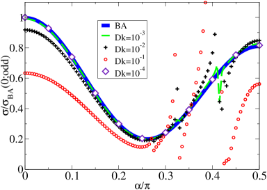
Figure 1: (Color Online) The Born approximation (BA) for fermions shown as a function of $\alpha/\pi$. We have plotted the energy independent: $\sigma/\sigma_{BA}^{odd}(\alpha=0)$ as a function of $\alpha$ for $Dk=10^{-1}$ (red open circle), $10^{-2}$ (blue +), $10^{-3}$ (green dash), $10^{-4}$ (purple open diamond), and the BA is shown as a bold blue line.

In the threshold regime the Born approximation (BA) offers a good estimate of the scattering for non-zero partial waves ticknor2d ; ajp_2d . This is most useful for estimating the cross section for identical fermions. In this model the dipoles are spinless and the way one models fermions or bosons is by imposing the symmetric or anti-symmetric requirement on the spatial wavefunction. This leads to the scattering properties of fermions being a sum of only the odd partial waves and bosons a sum of only the even. For the case of distinguishable particles, one sums up all of the partial waves. The BA result for this systems is:

$$k\sigma_{BA}^{m\rightarrow m}={4(Dk)^{2}\over(m^{2}-{1\over 4})^{2}}\left(1-{3\over 2}\sin(\alpha)^{2}\right)^{2}$$ (4)

$$k\sigma_{BA}^{\pm 1\rightarrow\mp 1}={4(Dk)^{2}\over(m^{2}-{1\over 4})^{2}}\left({3\over 4}\sin(\alpha)^{2}\right)^{2}$$

$$k\sigma_{BA}^{m\rightarrow m+2}={4(Dk)^{2}\over\left((m+{1\over 2})(m+{3\over 2})\right)^{2}}\left({3\over 4}\sin(\alpha)^{2}\right)^{2}$$

There are two basic types of collisions given here: diagonal and off-diagonal or $m$ changing. For the off-diagonal scattering, there is a special case of p-wave collisions where $\pm 1$ goes to $\mp 1$ and has the same functional form as the diagonal contribution. Then for the other off-diagonal terms $m\rightarrow m+2$, there is a distinct form. For identical fermions, the BA can be compared directly to the full scattering cross section with out worrying about a short range phase shift. This comparison is made in Fig. 1 where the full cross section is divided by the $\alpha=0$ BA cross section. Plotting this removes the energy dependence of the cross section. The BA is shown as a thick blue line normalized by its $\alpha=0$ value, and the full cross sections ares shown for $Dk=10^{-4}$ (violet open diamonds), $10^{-3}$ (dashed green), $10^{-2}$ (black $+$), and $0.1$ (red open circles). Relating $Dk$ to scattering energy is simply: $E/E_{D}=(Dk)^{2}/2$.

In Fig. 1 the agreement is good for the full range of $\alpha$, especially at small $k$. But it is worth noticing for $\rho_{0}/D=0.01$ there are two resonances as $\alpha/\pi$ goes to $1/2$. This are most clearly seen in $k=0.1$. For the smaller values of $k$ they are narrow and the region where the $\sigma$s deviates from the BA are increasingly small.

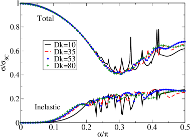
Figure 2: (Color Online) The total and inelastic $\sigma/\sigma_{SC}$ as a function of $\alpha$ is plotted for four different values of $Dk$: 10 (black solid line), 35 (red dashed), 53 (blue circles), and 80 (green +). The inelastic data is when $m$ is changed in a collisions, and in this case, it makes up a significant fraction of the scattering.

Alternatively, in the high energy regime we can estimate the cross section with the Eikonal Approximation ticknor2d : $\sigma_{SC}={4\over k}\sqrt{\pi Dk}$. This offers a good estimate of the scattering cross section. We have plotted the scattering cross section over $\sigma_{SC}$. Plotting this quantity removes the energy dependence of the scattering. In Fig. 2 we have plotted both the total and inelastic ($m$ changing) cross sections over $\sigma_{SC}$. The different energies are $k$=10 (black solid line), 35 (red dashed), 53 (blue circles), and 80 (green +). This estimate is given for the distinguishable case. In the case of bosons or fermions their $\sigma$ will oscillate about $\sigma_{Eik}$ ticknor2d ; jose . Notice that the elastic scattering never turns off even though there is no diagonal interaction at $\alpha_{c}/\pi\sim 0.30$. This shows that the scattering is made up from second-order processes; even though there is no diagonal interaction, there is a significant diagonal scattering contribution because of the off-diagonal channel couplings. The shape of this curve is that the total scattering rate dips and reduces to about 40$\%$ of it original value then increases up to about 65$\%$. The inelastic rate starts at zero and quickly climbs until $\alpha/\pi>0.2$, but after that it only slightly increases. For the lower end of this regime ($k=10$) scattering, there are still noticeable resonances in the scattering when a single partial wave makes up a large percentage of the scattering.

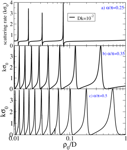
Figure 3: (Color Online) The scattering rate, $k\sigma_{0}$, as a function of $\rho_{0}/D$ at three different angles: a) $\alpha/\pi=0.25$, b) $\alpha/\pi=0.35$, and c) $\alpha/\pi=0.50$ at $Dk=10^{-2}$ (black). Notice that these resonances for small angles are narrow and fewer in number than the case where polarization is in-plane. In that case there are many resonances and they are wider in $\rho_{0}/D$.

With these simple estimates of the scattering magnitude in hand, we now move to study the impact of the tilted polarization axis on the scattering for bosons or distinguishable dipoles, where there is the $m=0$ contribution relaying information about the short range scattering. For fermions, the short-range is strongly shielded, and only when one considers specific cases does the scattering become more involved. For this reason, we are more interested in the bosonic scattering and general long-range behavior and leave the case specific fermionic scattering for the future.

As a first look at this scattering behavior, we look at the scattering rate as a function of $\rho_{0}/D$ at three different angles: a) $\alpha/\pi=0.25$, b) $\alpha/\pi=0.35$, and c) $\alpha/\pi=0.50$. In Fig. 3 a) the resonances which occur as $\rho_{0}/D$ is decreased are narrow. Only a few exist because there is a dipolar barrier to the scattering and thus the inter-channel couplings at short range must be strong enough to support the bound state. As the polarization angle is increased, the resonances become wider and more frequent. As the barrier is turned off and ultimately turning into an attractive potential, we see more frequent and wide resonances. These resonances are much like the long range resonances seen in 3D You ; CTPR ; NJP ; universal ; roudnev ; kanj2 .

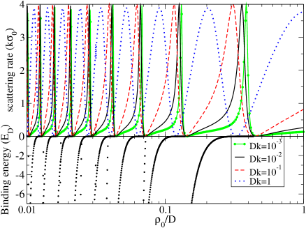
Figure 4: (Color Online) Energy dependence of the scattering rate, $k\sigma_{0}$ and the binding energies are shown as a function of $\rho_{0}/D$ for $\alpha/\pi=0.35$. The curves are for $Dk=10^{-3}$ (green with circles), $10^{-2}$ (black), $10^{-1}$ (dashed red) and $1$ (blue dotted). The binding energies are also shown for the same $\rho_{0}/D$. The cross sections and binding energy go to zero simultaneously and the strong energy dependence of the scattering resonance width.

To study this energy dependence of the scattering further, we look at a particular angle and vary the energy. In Fig. 4 we have plotted the scattering rate ($\alpha/\pi=0.35$) in the upper panel at four values of $Dk$: $10^{-3}$ (green with circles), $10^{-2}$ (black), $10^{-1}$ (dashed red) and $1$ (blue dotted). In the lower panel we have plotted the binding energy. There are a few points to be made here about the strong energy dependence of the scattering. First, the peak of the resonance shifts noticeably as the energy is lowered. Second, the width of the resonance becomes more narrow as the energy is decreased. Third, as the the binding energy goes to zero, the scattering rate goes to zero; this is in contrast to 3D. Fourth, for the $|m|>0$ resonances are very narrow, and they bind tightly as $\rho_{0}/D$ is decreased. In these plots these resonance are hard to see because they are so narrow. They are most easily found by looking at the binding energy where there are steep lines.

It is worth commenting on the relationship between the scattering length and the cross section and how these two quantities relate to the binding energy. First, for identical bosons in 3D, the cross section is $\sigma\sim 8\pi a^{2}$ but for $a\gg k$ it saturates at $8\pi/k^{2}$. In the large $a$ limit, the binding energy goes as $\left(-{\hbar^{2}\over 2\mu a^{2}}\right)$, and the maximum of $a$ corresponds to the maximum of $\sigma$. 2D is very different. Consider when $a\rightarrow\infty$, and the scattering cross section goes to zero. This is most easily seen as from the effective range expansion: $\cot(\delta)\propto\ln(ka)\rightarrow\infty$. This leads to $\delta\sim 0$ and $\sigma\sim 0$ when $a$ is very large. The maximum of the scattering cross section occurs at $\delta=\pi/2$, and this happens when $ak=2e^{-\gamma}\sim 1.12$.

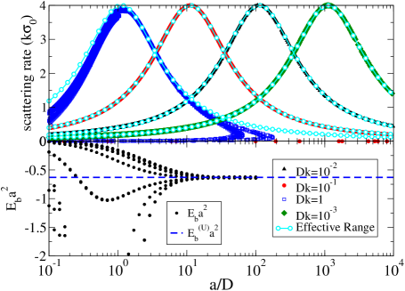
Figure 5: (Color Online) The scattering rate, $k\sigma_{0}$, and $a^{2}E_{b}$ are shown as a function of $a$ for many values of $\alpha$. The different energies are: $Dk=10^{-3}$ (green), $10^{-2}$ (black) $10^{-1}$ (red) and $1$ (blue). Cyan open circles are the effective range at each energy. The energy dependence of the scattering rate is seen simply as where the scattering rate peaks when $ka=2e^{-\gamma}\sim 1.12$. The binding energies times $a^{2}$ are also shown for all resonances, the blue dashed line is the universal limit, $\sim 0.63$. Only for the $Dk=1$ does the effective range not give a good estimate of the scattering rate.

A way to clearly demonstrate the energy dependent behavior is shown in Fig. 5, where we have replotted the scattering rate and binding energy as a function of $a/D$, not $\rho_{0}/D$. We have replotted all the scattering data (i.e. many different values of $\alpha$) as a function of $a/D$ for many different values of $Dk$: $10^{-3}$ (black), $10^{-2}$ (red) $10^{-1}$ (green) and $1$ (blue). The binding energies are now plotted as $a^{2}E_{b}$, this makes it so that when the energies become universal they go to a constant value of $\sim$-0.63. Replotting the data this way, allows us to observe clearly several points. First, the scattering rate is maximum when $ka=2e^{-\gamma}\sim 1.12$; this is clear from the four different energies plotted. It is also clear that the 2D system has strong energy dependence, and that the scattering rate goes to zero in the large $a$ limit.

From this plot we can understand why there is such strong energy dependence to the width of the resonances as a function of $\rho_{0}/D$. $a/D$ is energy independent once one is in the threshold regime and depends only on $\rho_{0}/D$. We know that the scattering rate is zero when $a\rightarrow\infty$ and that it is maximum when $ka\sim 1.12$. Therefore as energy is decreased, the maximum and minimum of the scattering rate approach each other in $a/D$ (Fig. 5) or $\rho_{0}/D$ (Fig 4).

The effective range expansion gives a very good estimate of the scattering rate and therefore the phase shift at low $k$. For $k$=1 (blue squares), we are leaving the threshold regime, and the effective range description breaks down.

Moving to the binding energies, we are see $a^{2}E_{b}$ (black circles) converges to the universal value (blue dashed line) for $a/D>10$ and when it is strongly system dependent. We also see that at small $a/D$ the binding energies deviate from the universal trend and $a^{2}E_{b}$ widely varies. In this figure we have only plotted the binding energies which were numerically found. Going beyond $a/D$=100 is both computationally challenging and only returns the universal binding energy.

IV Molecules

In this system the molecules have widely varying properties depending on the polarization angle. To study them more closely we pick six angles to explore: $\alpha/\pi$=0.25, 0.275, 0.3, 0.35, 0.4, and 0.5. For $\alpha/\pi$ smaller than 0.2, very little variation in the scattering, and there are no bound states for the values of $\rho_{0}/D$ we consider. The first important point is that for a given angle the properties are robust. This is demonstrated by obtaining the molecular energies and wavefunctions for the first two $m=0$ resonances for each angle. Then we determine the values of $\rho_{0}/D$ at each resonance which result in a set of chosen scattering lengths. We pick 40 different scattering lengths between 0.1 and 100$D$ that are found at each of the first 2 resonances for each of the 6 angles.

This idea of using $a/D$ as the control parameter was used in 3D dipolar scattering to study three body recombination of dipoles 3body . That work showed that using the scattering length to characterize the 2-body system in the calculations, even outside the $a\gg D$ regime, worked well at revealing universal characteristics of three body recombination.

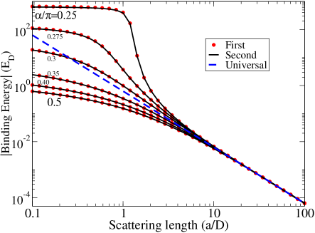
Figure 6: (Color Online) The binding energies for the first and second $m=0$ resonances at $\alpha/\pi$= 0.25, 0.275, 0.3, 0.35, 0.4, and 0.5. The universal 2D binding energy at large $a/D$ is shown as a blue dashed line.

In fig. 6 we plot the binding energies of the molecules for the first (black line) and second (red circle) resonance for all values of $\alpha$ considered. For $\alpha/\pi=0.25$ the molecules are most tightly bound at small $a/D$ and at $\alpha/\pi=0.5$ are most loosely bound, as expected, although there is roughly 2 orders of magnitude difference in the binding energies between these two extreme cases. For the tightly bound case the binding energies plateau as $a/D$ is lowered. This energy corresponds to the size of the hard sphere and therefore a minimum size of the molecule. In this case there is a strong dipolar barrier and it is the inter-channel couplings that form the attractive short range region where the molecule is found. In contrast for $\alpha/\pi=0.5$ there is an attractive dipolar term for the $m=0$ case and the molecules are only mildly multi-channel objects. This will be explained below.

As $a/D$ is increased, for all of the polarization angles, the system becomes more loosely bound, and they are strongly system dependent. Only for relatively large $a/D$, say 10, do the binding energies truly resemble the universal value. We have plotted the universal binding energy as a blue dashed line.

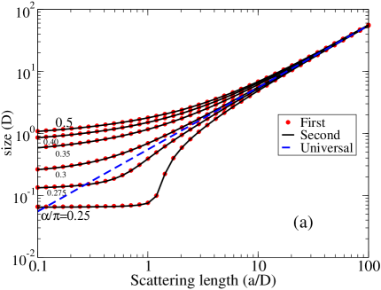
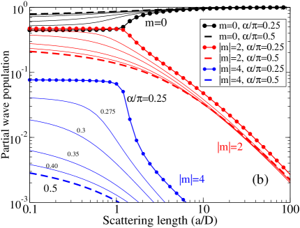
Figure 7: (Color Online) (a) The size of the molecules are shown as a function of $a/D$ for various angles for both the first (black) and second (red circles) resonance. The universal form of the size is shown as a dashed blue line. (b) The partial wave population is shown (first resonance only), for all six angles as a function of $a/D$. The extreme angles are shown as filled circles ($\alpha/\pi=0.25$) and dashed lines ($\alpha/\pi=0.5$) for partial waves $m=0$ (black), $|m|=2$ (red) and $|m|=4$ (blue).

We now consider the size and shape of the molecules. First in Fig. 7 (a) we look at the expectation value of the molecular size: $\langle\psi|\rho|\psi\rangle$ as a function of scattering length. All values of $\alpha$ are plotted for both the first (black line) and second (red circle) resonance. For $\alpha/\pi=0.25$ and small $a/D$ the molecules are very small, $\langle\rho\rangle\sim 0.05D$; this is roughly the size of the hard sphere when the first bound state is captured. In contrast $\alpha/\pi=0.5$ the molecule is about $\langle\rho\rangle\sim 1D$ even for $a/D\sim 0.1$. In the large $a/D$ limit we find that the size of the molecule goes to $\pi^{2}e^{\gamma}a/32\sim 0.55a$ (blue dashed) which was obtained from $\phi_{b}(\kappa_{a}\rho)$. Again we find that the size of the molecules depends on the polarization until $a/D>10$.

Now we look at the shape of the molecules shown in Fig. 7 (b). This is done by considering the partial wave population $n_{m}=\langle\phi_{m}|\phi_{m}\rangle$ as a function of scattering length for each angle. The extreme angles of $\alpha/\pi=0.25$ and $\alpha/\pi=0.5$ are shown as filled circles and dashed lines for $m=0$ (black), $|m|=2$ (red) and $|m|=4$ (blue).

For $\alpha/\pi=0.25$ and small $a/D$ the molecules are strongly aligned along the polarization axis behind the dipolar barrier. This is why they are so small and highly aligned. This is seen by the fact that the largest contribution is from $|m|=2$ (red circles) and $|m|=4$ (blue circles) is nearly 10$\%$ of the partial wave population at small scattering length. This is from the fact that the dipoles are behind the dipolar barrier and the inter-channel couplings are the origin of the molecule. The anisotropy at small $a/D$ is still true for $\alpha/\pi=0.5$, but the $m$=0 contribution is nearly 80$\%$. This strong contrast is from because of the attractive dipolar interaction for the $m=0$ channel only requires a slight amount of inter-channel coupling to form a bound state. For the 3D case, the $l=0$ molecule is made up of about about 60$\%$ s-wave and the rest is essentially d-wave 3body .

It is important to notice that at large $a/D$ the partial wave populations go to very similar values. The $m=0$ contribution dominates and all other contributions become small. To better understand the shape of the molecules we plot the radial weighted molecular densities.

Figure 8: (Color Online) $\rho|\psi(\vec{\rho})|^{2}$ for: $\alpha/\pi=$ a) 0.25, b) 0.35, c) 0.5 for $a/D$ (i) 0.1, (ii) 1, (iii) 10 and (iv) 100. The contours indicated are drawn ever 20$\%$ of maximum value, with the largest 80$\%$ contour being drawn as red. The solid grey circle in the middle is the hard sphere short range interaction. The scale changes for every plot on the left (i, ii), in contrast the scale is the same for the plots on the right (iii, iv) when the system is in the large $a/D$ regime.

In Fig. 8 we have plotted the radial weighted molecular densities: $\rho|\psi(\vec{\rho})|^{2}=|\sum_{m}u_{m}(\rho)e^{im\phi}|^{2}$ for $\alpha/\pi=$ a) 0.25, b) 0.35, c) 0.5 (top to bottom) for $a/D$ of (i) 0.1, (ii) 1, (iii) 10, and (iv) 100 (left to right). These densities are generated from the second resonance. The first resonance wavefunctions look the same expect there inner hard core is larger and over takes the inner oscillations. The scale changes for the plots on the left.

This plot clearly shows the change in both shape and size of the molecules as both $a/D$ and $\alpha/\pi$ are changed. Now starting at $a/D=0.1$ and $\alpha/\pi$=0.25 (ai) we see that the molecule is very small and highly anisotropic. The density is along the polarization axis, $x$, and very tightly bound against the hard core. In fact its spatial extend does not really extend beyond the hard core in the $y$ direction.

Then as the angle is increased, for a fixed $a/D$ the size of the molecule and anisotropy is softened. Observe the change is scale in both (bi) and (ci). In (ci), the molecule is larger ($\sim 1D$), and still aligned along the polarization axis. Additionally see the contrast in (ai) and (ci) between the extend of the density over the width in $y$ of the hard core.

Now for (a), (b), and (c) consider increasing $a/D$. The size of the molecules gets larger and more isotropic. In (iv) for all angles the system is isotropic, except for small region near the hard core, but the bulk of the radial weighted density is isotropically distributed at large $\rho$. This is why the size and shape of the molecules are universal in the large $a/D$ limit.

V Conclusions

In this paper we have studied the scattering properties of the a pure 2D dipolar system when the polarization can tilt into the plane of motion. We have shown how the tilt angle impacts the scattering in both the threshold and semi-classical regimes. We then studied the character of the scattering resonances generated by altering $\rho_{0}/D$ or electric field as a function of the polarization angle. We found that at small angles the systems gained bound states which produced narrow resonances. This is because of the dipolar barrier. We also found when the polarization is entirely in the plane of motion, the resonances are frequent and wide because of the partially attractive potential.

We studied the molecular system generated the tilt of the polarization. We showed that at large $a/D$ the system have a universal shape independent of polarization angle, but at small $a/D$ we have found that the molecules have a wide range of properties which strongly depend on polarization angle. Future work on this topic will be to more fully consider a realistic system, to include the effect of confinement, fermionic dipoles and layer systems.

- (1) #
- (2) M. A. Baranov, Phys. Rep. 464 71 (2008).
- (3) L. D. Carr et al. New J. Phys. 11, 055049 (2009).
- (4) M. H. G. de Miranda et al., 1 Nat. Phys. (2011).
- (5) S. Ospelkaus et al. Science 327, 853 (2010).
- (6) P. S. Zuchowski and J. M. Hutson, Phys. Rev. A 81, 060703 (2010).
- (7) C. Ticknor, R.M.Wilson, and J.L. Bohn, Phys. Rev. Lett. 106, 065301 (2011).
- (8) G. M. Bruun and E. Taylor, Phys. Rev. Lett. 101, 245301 (2008).
- (9) J. C. Cremon, G. M. Bruun, and S. M. Reimann, Phys. Rev. Lett. 105, 255301 (2010).
- (10) C. Ticknor, Phys. Rev. A. 80 052702 (2009).
- (11) C. Ticknor, Phys. Rev. A. 81 042708 (2010).
- (12) J. D’Incao and C. H. Greene, Phys. Rev. A 83, 030702(R) (2011).
- (13) G. Quemener and J. L. Bohn, Phys. Rev. A 81, 060701 (2010); 83 012705 (2011).
- (14) A. Micheli et al. Phys. Rev. Lett. 105, 073202 (2010).
- (15) M. Klawunn, A. Pikovski and L. Santos, Phys. Rev. A 82, 044701 (2010)
- (16) J. R. Armstrong, N. T. Zinner, D. V. Fedorov, and A. S. Jensen, Europhysics Letters 91, 16001 (2010).
- (17) A. G. Volosniev, D. V. Fedorov, A. S. Jensen, and N. T. Zinner, ArXiv1103.1549.
- (18) B. J. Verhaar, et al., J. Phys. A: Math. Gen. 17, 595 (1984).
- (19) K. Kanjilal and D. Blume, Phys. Rev. A 73, 060701 (2006).
- (20) B. R. Johnson, J. Comput. Phys. 13, 445 (1973).
- (21) Z.-Y. Gu and S. W. Quian, Phys. Lett. A 136, 6 (1989).
- (22) I. R. Lapidus, Am. J. Phys. 50, 45 (1982); S. K. Adhikari, Am. J. Phys. 54, 362 (1986).
- (23) C. Ticknor, Phys. Rev. Lett., 100 133202 (2008); Phys. Rev. A 76, 052703 (2007).
- (24) V. Roudnev and M. Cavagnero, Phys. Rev. A, 79 014701 (2009); J. Phys. B, 42, 044017 (2009).
- (25) J. L. Bohn, M. Cavagnero, and C. Ticknor, New J. Phys. 11 055039 (2009).
- (26) K. Kanjilal and D. Blume, Phys. Rev. A 78, 040703(R) (2008).
- (27) M. Marinescu and L. You, Phys. Rev. Lett. 81, 4596 (1998).
- (28) C. Ticknor and J. L. Bohn Phys. Rev. A 72, 032717 (2005).
- (29) C. Ticknor and S. T. Rittenhouse, Phys. Rev. Lett. 105, 013201 (2010).