Possible Deuteron-like Molecular States Composed of Heavy Baryons

Abstract

We perform a systematic study of the possible loosely bound states composed of two charmed baryons or a charmed baryon and an anti-charmed baryon within the framework of the one boson exchange (OBE) model. We consider not only the $\pi$ exchange but also the $\eta$, $\rho$, $\omega$, $\phi$ and $\sigma$ exchanges. The $S-D$ mixing effects for the spin-triplets are also taken into account. With the derived effective potentials, we calculate the binding energies and root-mean-square (RMS) radii for the systems $\Lambda_{c}\Lambda_{c}(\bar{\Lambda}_{c})$, $\Xi_{c}\Xi_{c}(\bar{\Xi}_{c})$, $\Sigma_{c}\Sigma_{c}(\bar{\Sigma}_{c})$, $\Xi_{c}^{\prime}\Xi_{c}^{\prime}(\bar{\Xi}_{c}^{\prime})$ and $\Omega_{c}\Omega_{c}(\bar{\Omega}_{c})$. Our numerical results indicate that: (1) the H-dibaryon-like state $\Lambda_{c}\Lambda_{c}$ does not exist; (2) there may exist four loosely bound deuteron-like states $\Xi_{c}\Xi_{c}$ and $\Xi_{c}^{\prime}\Xi_{c}^{\prime}$ with small binding energies and large RMS radii. .

I Introduction

Many so-called “XYZ” charmonium-like states such as $X(3872)$, $X(4350)$ and $Y(3940)$ have been observed by Belle, CDF, D0 and BaBar collaborations Belle ; BaBar ; CDF ; D0 during the past few years. Despite the similar production mechanism, some of these structures do not easily fit into the conventional charmonium spectrum, which implies other interpretations such as hybrid mesons, heavy meson molecular states etc. might be responsible for these new states Brambilla:2010cs Swanson2006 .

A natural idea is that some of the “XYZ” states near two heavy meson threshold may be bound states of a pair of heavy meson and anti-heavy meson. Actually, Rujula et al. applied this idea to explain $\psi(4040)$ as a P-wave $D^{*}\bar{D}^{*}$ bound resonance in the 1970s Rujula77 . Tornqvist performed an intensive study of the possible deuteron-like two-charm-meson bound states with the one-pion-exchange (OPE) potential model in Ref. Torq . Recently, motivated by the controversy over the nature of $X(3872)$ and $Z(4430)$, some authors proposed $X(3872)$ might be a $D\bar{D}^{*}$ bound state Swan04 ; Wong04 ; Close2004 ; Voloshin2004 ; Thomas2008 . Our group have studied the possible molecular structures composed of a pair of heavy mesons in the framework of the One-Boson-Exchange (OBE) model systematically LiuXLiuYR ; ZhugrpDD . There are also many interesting investigations of other hadron clusters Ding ; LiuX ; Liu2009 ; Ping:2000dx ; Liu:2011xc ; qiao .

The boson exchange models are very successful to describe nuclear force Mach87 ; Mach01 ; Rijken . Especially the deuteron is a loosely bound state of proton and neutron, which may be regarded as a hadronic molecular state. One may wonder whether a pair of heavy baryons can form a deuteron-like bound state through the light meson exchange mechanism. On the other hand, the large masses of the heavy baryons reduce the kinetic of the systems, which makes it easier to form bound states. Such a system is approximately non-relativistic. Therefore, it is very interesting to study whether the OBE interactions are strong enough to bind the two heavy baryons (dibaryon) or a heavy baryon and an anti-baryon (baryonium).

A heavy charmed baryon contains a charm quark and two light quarks. The two light quarks form a diquark. Heavy charmed baryons can be categorized by the flavor wave function of the diquark, which form a symmetric $6$ or an antisymmetric $\bar{3}$ representation. For the ground heavy baryon, the spin of the diquark is either $0$ or $1$, and the spin of the baryon is either $1/2$ or $3/2$. The product of the diquark flavor and spin wave functions of the ground charmed baryon must be symmetric and correlate with each other. Thus the spin of the sextet diquark is $1$ while the spin of the anti-triplet diquark is $0$.

The ground charmed baryons are grouped into one antitrpilet with spin-1/2 and two sextets with spin-1/2 and spin-3/2 respectively. These multiplets are usually denoted as $B_{\bar{3}}$, $B_{6}$ and $B_{6}^{*}$ in literature Yan . In the present work, we study the charmed dibaryon and baryonium systems, i.e. $\Lambda_{c}\Lambda_{c}(\bar{\Lambda}_{c})$, $\Xi_{c}\Xi_{c}(\bar{\Xi}_{c})$, $\Sigma_{c}\Sigma_{c}(\bar{\Sigma}_{c})$, $\Xi^{\prime}_{c}\Xi^{\prime}_{c}(\bar{\Xi}_{c}^{\prime})$ and $\Omega_{c}\Omega_{c}(\bar{\Omega}_{c})$. Other configurations will be explored in a future work. We first derive the effective potentials of these systems. Then we calculate the binding energies and root-mean-square (RMS) radii to determine which system might be a loosely bound molecular state.

This work is organized as follows. We present the formalism in section II. In section III, we discuss the extraction of the coupling constants between the heavy baryons and light mesons and give the numerical results in Section IV. The last section is a brief summary. Some useful formula and figures are listed in appendix.

II Formalism

In this section we will construct the wave functions and derive the effective potentials.

II.1 Wave Functions

As illustrated in Fig. 1, the states $\Lambda_{c}^{+}$, $\Xi_{c}^{+}$ and $\Xi_{c}^{0}$ belong to the antitriplet $B_{\bar{3}}$ while $\Sigma_{c}^{++}$, $\Sigma_{c}^{+}$, $\Sigma_{c}^{0}$, $\Xi_{c}^{\prime+}$, $\Xi_{c}^{\prime 0}$ and $\Omega_{c}^{0}$ are in sextet $B_{6}$. Among them, $\Lambda_{c}^{+}$ and $\Omega_{c}^{0}$ are isoscalars; $\{\Xi_{c}^{+},\Xi_{c}^{0}\}$ and $\{\Xi_{c}^{\prime+},\Xi_{c}^{\prime 0}\}$ are isospin spinnors; $\{\Sigma_{c}^{++},\Sigma_{c}^{+},\Sigma_{c}^{0}\}$ is an isovector. We denote these states $\Lambda_{c}$, $\Xi_{c}$, $\Sigma_{c}$, $\Xi_{c}^{\prime}$ and $\Omega_{c}$.

(a) antitriplet

(b) sextet

Figure 1: The antitriplet and sextet. Here the brackets and parentheses represent antisymmetrization and symmetrization of the light quarks respectively.

The wave function of a dibaryon is the product of its isospin, spatial and spin wave functions,

$$\Psi_{hh}^{[I,2S+1]}\sim\Psi_{hh}^{I}\otimes\Psi_{hh}^{L}\otimes\Psi_{hh}^{S}.$$ (1)

We consider the isospin function $\Psi_{hh}^{I}$ first. The isospin of $\Lambda_{c}$ is $0$, so $\Lambda_{c}\Lambda_{c}$ has isospin $I=0$ and $\Psi_{\Lambda_{c}\Lambda_{c}}^{I=0}=\Lambda_{c}^{+}\Lambda_{c}^{+}$, which is symmetric. For $\Xi_{c}\Xi_{c}$, the isospin is $I=0$ or $1$, and their corresponding wave functions are antisymmetric and symmetric respectively. $\Sigma_{c}\Sigma_{c}$ has isospin $0$, $1$ or $2$. Their flavor wave functions can be constructed using Clebsch-Gordan coefficients. $\Xi_{c}^{\prime}\Xi_{c}^{\prime}$ is the same as $\Xi_{c}\Xi_{c}$. The isospin of the $\Omega_{c}\Omega_{c}$ is $0$. Because strong interactions conserve isospin symmetry, the effective potentials do not depend on the third components of the isospin. For example, it is adequate to take the isospin function $\Xi_{c}^{+}\Xi_{c}^{+}$ with $I_{3}=1$ when we derive the effective potential for $\Psi_{\Xi_{c}\Xi_{c}}^{I=1}$, though the wave function $\frac{1}{\sqrt{2}}(\Xi_{c}^{+}\Xi_{c}^{0}+\Xi_{c}^{0}\Xi_{c}^{+})$ indeed gives the same result. In the following, we show the relevant isospin functions used in our calculation,

$$\Psi_{\Lambda_{c}\Lambda_{c}}^{I=0} = \Lambda_{c}^{+}\Lambda_{c}^{+}$$ (2)

$$\Psi_{\Xi_{c}\Xi_{c}}^{I=0} = \frac{1}{\sqrt{2}}\left(\Xi_{c}^{+}\Xi_{c}^{0}-\Xi_{c}^{0}\Xi_{c}^{+}\right)$$

$$\Psi_{\Xi_{c}\Xi_{c}}^{I=1} = \Xi_{c}^{+}\Xi_{c}^{+}$$ (3)

$$\Psi_{\Sigma_{c}\Sigma_{c}}^{I=0} = \frac{1}{\sqrt{3}}\left(\Sigma_{c}^{++}\Sigma_{c}^{0}-\Sigma_{c}^{+}\Sigma_{c}^{+}+\Sigma_{c}^{0}\Sigma_{c}^{++}\right)$$

$$\Psi_{\Sigma_{c}\Sigma_{c}}^{I=1} = \frac{1}{\sqrt{2}}\left(\Sigma_{c}^{++}\Sigma_{c}^{+}-\Sigma_{c}^{+}\Sigma_{c}^{++}\right)$$

$$\Psi_{\Sigma_{c}\Sigma_{c}}^{I=2} = \Sigma_{c}^{++}\Sigma_{c}^{++}$$ (4)

$$\Psi_{\Xi_{c}^{\prime}\Xi_{c}^{\prime}}^{I=0} = \frac{1}{\sqrt{2}}\left(\Xi_{c}^{\prime+}\Xi_{c}^{\prime 0}-\Xi_{c}^{\prime 0}\Xi_{c}^{\prime+}\right)$$

$$\Psi_{\Xi_{c}^{\prime}\Xi_{c}^{\prime}}^{I=1} = \Xi_{c}^{\prime+}\Xi_{c}^{\prime+}$$ (5)

$$\Psi_{\Omega_{c}\Omega_{c}}^{I=0} = \Omega_{c}^{0}\Omega_{c}^{0}.$$ (6)

We are mainly interested in the ground states of dibaryons and baryonia where the spatial wave functions of these states are symmetric. The tensor force in the effective potentials mixes the $S$ and $D$ waves. Thus a physical ground state is actually a superposition of the $S$ and $D$ waves. This mixture fortunately does not affect the symmetries of the spatial wave functions. As a mater of fact, for a dibaryon with a specific total spin $\bm{J}$, we must add the spins of its components to form $\bm{S}$ first and then couple $\bm{S}$ and the relative orbit angular momentum $\bm{L}$ together to get $\bm{J}=\bm{L}+\bm{S}$. This $L-S$ coupling scheme leads to six $S$ and $D$ wave states: ${}^{1}S_{0}$, ${}^{3}S_{1}$, ${}^{1}D_{2}$, ${}^{3}D_{1}$, ${}^{3}D_{2}$ and ${}^{3}D_{3}$. But the tenser force only mixes states with the same $S$ and $J$. In our case we must deal with the ${}^{3}S_{1}$-${}^{3}D_{1}$ mixing. After stripping off the isospin function, the mixed wave function is

$$|\psi\rangle=R_{S}(r)|^{3}S_{1}\rangle+R_{D}(r)|^{3}D_{1}\rangle,$$ (7)

which will lead to coupled channel Schrödinger equations for the radial functions $R_{S}(r)$ and $R_{D}(r)$. In short, for the spatial wave functions, we will discuss the ground states in ${}^{1}S_{0}$ and ${}^{3}S_{1}$, and the latter mixes with ${}^{3}D_{1}$.

Finally, we point out that the $I$ and $S$ of states in Eq. (1) can not be combined arbitrarily because the generalized identity principle constricts the wave functions to be antisymmetric. It turns out that the survived compositions are $\Psi_{\Lambda_{c}\Lambda_{c}}^{[0,1]}$, $\Psi_{\Xi_{c}\Xi_{c}}^{[0,3]}$, $\Psi_{\Xi_{c}\Xi_{c}}^{[1,1]}$, $\Psi_{\Sigma_{c}\Sigma_{c}}^{[0,1]}$,$\Psi_{\Sigma_{c}\Sigma_{c}}^{[1,3]}$,$\Psi_{\Sigma_{c}\Sigma_{c}}^{[2,1]}$,$\Psi_{\Xi_{c}^{\prime}\Xi_{c}^{\prime}}^{[0,3]}$, $\Psi_{\Xi_{c}^{\prime}\Xi_{c}^{\prime}}^{[1,1]}$, and $\Psi_{\Omega_{c}\Omega_{c}}^{[0,1]}$. For baryonia, there is no constraint on the wave functions. So we need take into account more states. The wave functions of baryonia can be constructed in a similar way. However, we can use the so-called “G-Parity rule” to derive the effective potentials for baryonia directly from the corresponding potentials for dibaryons, and it is no need discussing them here now.

II.2 Lagrangians

We introduce notations

$$\Lambda_{c}=\Lambda_{c}^{+},\quad\Xi_{c}=\left(\begin{array}[]{c}\Xi_{c}^{+}\\ \Xi_{c}^{0}\end{array}\right),\quad\bm{\Sigma}_{c}=\left\{\frac{1}{\sqrt{2}}(-\Sigma_{c}^{++}+\Sigma_{c}^{0}),\frac{i}{\sqrt{2}}(-\Sigma_{c}^{++}-\Sigma_{c}^{0}),\Sigma_{c}^{+}\right\},\quad\Xi_{c}^{\prime}=\left(\begin{array}[]{c}\Xi_{c}^{\prime+}\\ \Xi_{c}^{\prime 0}\end{array}\right),\quad\Omega_{c}=\Omega_{c}^{0}$$ (12)

to represent the corresponding baryon fields. The long range interactions are provided by the $\pi$ and $\eta$ meson exchanges:

$$\mathcal{L}_{\pi} = g_{\pi\Xi_{c}\Xi_{c}}\bar{\Xi}_{c}i\gamma_{5}\bm{\tau}\Xi_{c}\cdot\bm{\pi}+g_{\pi\Sigma_{c}\Sigma_{c}}(-i)\bar{\bm{\Sigma}}_{c}i\gamma_{5}\times\bm{\Sigma}_{c}\cdot\bm{\pi}+g_{\pi\Xi_{c}^{\prime}\Xi_{c}^{\prime}}\bar{\Xi}^{\prime}_{c}i\gamma_{5}\bm{\tau}\Xi^{\prime}_{c}\cdot\bm{\pi}$$ (13)

$$\mathcal{L}_{\eta} = g_{\eta\Lambda_{c}\Lambda_{c}}\bar{\Lambda}_{c}i\gamma_{5}\Lambda_{c}\eta+g_{\eta\Xi_{c}\Xi_{c}}\bar{\Xi}_{c}i\gamma_{5}\Xi_{c}\eta$$ (14)

$$+g_{\eta\Sigma_{c}\Sigma_{c}}\bar{\bm{\Sigma}}_{c}\cdot i\gamma_{5}\bm{\Sigma}_{c}\eta+g_{\eta\Xi_{c}^{\prime}\Xi_{c}^{\prime}}\bar{\Xi}_{c}^{\prime}i\gamma_{5}\Xi_{c}^{\prime}\eta+g_{\eta\Omega_{c}\Omega_{c}}\bar{\Omega}_{c}i\gamma_{5}\Omega_{c}\eta,$$

where $g_{\pi\Xi_{c}\Xi_{c}}$, $g_{\pi\Sigma_{c}\Sigma_{c}}$, $g_{\eta\Omega_{c}\Omega_{c}}$ etc. are the coupling constants. $\bm{\tau}=\{\tau_{1},\tau_{2},\tau_{3}\}$ are the Pauli matrices, and $\bm{\pi}=\{\frac{1}{\sqrt{2}}(\pi^{+}+\pi^{-}),\frac{i}{\sqrt{2}}(\pi^{+}-\pi^{-}),\pi^{0}\}$ are the $\pi$ fields. The vector meson exchange Lagrangians read

$$\mathcal{L}_{\rho} = g_{\rho\Xi_{c}\Xi_{c}}\bar{\Xi}_{c}\gamma_{\mu}\bm{\tau}\Xi_{c}\cdot\bm{\rho}^{\mu}+\frac{f_{\rho\Xi_{c}\Xi_{c}}}{2m_{\Xi_{c}}}\bar{\Xi}_{c}\sigma_{\mu\nu}\bm{\tau}\Xi_{c}\cdot\partial^{\mu}\bm{\rho}^{\nu}$$ (15)

$$+g_{\rho\Sigma_{c}\Sigma_{c}}(-i)\bar{\bm{\Sigma}}_{c}\gamma_{\mu}\times\bm{\Sigma}_{c}\cdot\bm{\rho}^{\mu}+\frac{f_{\rho\Sigma_{c}\Sigma_{c}}}{2m_{\Sigma_{c}}}(-i)\bar{\bm{\Sigma}}_{c}\sigma_{\mu\nu}\times\bm{\Sigma}_{c}\cdot\partial^{\mu}\bm{\rho}^{\nu}$$

$$+g_{\rho\Xi_{c}^{\prime}\Xi_{c}^{\prime}}\bar{\Xi}_{c}^{\prime}\gamma_{\mu}\bm{\tau}\Xi_{c}^{\prime}\cdot\bm{\rho}^{\mu}+\frac{f_{\rho\Xi_{c}^{\prime}\Xi_{c}^{\prime}}}{2m_{\Xi^{\prime}_{c}}}\bar{\Xi}_{c}^{\prime}\sigma_{\mu\nu}\bm{\tau}\Xi_{c}^{\prime}\cdot\partial^{\mu}\bm{\rho}^{\nu}$$

$$\mathcal{L}_{\omega} = g_{\omega\Lambda_{c}\Lambda_{c}}\bar{\Lambda}_{c}\gamma_{\mu}\Lambda_{c}\omega^{\mu}+\frac{f_{\omega\Lambda_{c}\Lambda_{c}}}{2m_{\Lambda_{c}}}\bar{\Lambda}_{c}\sigma_{\mu\nu}\Lambda_{c}\partial^{\mu}\omega^{\nu}$$ (16)

$$+g_{\omega\Xi_{c}\Xi_{c}}\bar{\Xi}_{c}\gamma_{\mu}\Xi_{c}\omega^{\mu}+\frac{f_{\omega\Xi_{c}\Xi_{c}}}{2m_{\Xi_{c}}}\bar{\Xi}_{c}\sigma_{\mu\nu}\Xi_{c}\partial^{\mu}\omega^{\nu}$$

$$+g_{\omega\Sigma_{c}\Sigma_{c}}\bar{\bm{\Sigma}}_{c}\gamma_{\mu}\cdot\bm{\Sigma}_{c}\omega^{\mu}+\frac{f_{\omega\Sigma_{c}\Sigma_{c}}}{2m_{\Sigma_{c}}}\bar{\bm{\Sigma}}_{c}\sigma_{\mu\nu}\cdot\bm{\Sigma}_{c}\partial^{\mu}\omega^{\nu}$$

$$+g_{\omega\Xi_{c}^{\prime}\Xi_{c}^{\prime}}\bar{\Xi}_{c}^{\prime}\gamma_{\mu}\Xi_{c}^{\prime}\omega^{\mu}+\frac{f_{\omega\Xi_{c}^{\prime}\Xi_{c}^{\prime}}}{2m_{\Xi_{c}^{\prime}}}\bar{\Xi}_{c}^{\prime}\sigma_{\mu\nu}\Xi_{c}^{\prime}\partial^{\mu}\omega^{\nu}$$

$$\mathcal{L}_{\phi} = g_{\phi\Xi_{c}\Xi_{c}}\bar{\Xi}_{c}\gamma_{\mu}\Xi_{c}\phi^{\mu}+\frac{f_{\phi\Xi_{c}\Xi_{c}}}{2m_{\Xi_{c}}}\bar{\Xi}_{c}\sigma_{\mu\nu}\Xi_{c}\partial^{\mu}\phi^{\nu}$$ (17)

$$+g_{\phi\Xi_{c}^{\prime}\Xi_{c}^{\prime}}\bar{\Xi}_{c}^{\prime}\gamma_{\mu}\Xi_{c}^{\prime}\phi^{\mu}+\frac{f_{\phi\Xi_{c}^{\prime}\Xi_{c}^{\prime}}}{2m_{\Xi_{c}^{\prime}}}\bar{\Xi}_{c}^{\prime}\sigma_{\mu\nu}\Xi_{c}^{\prime}\partial^{\mu}\phi^{\nu}$$

$$+g_{\phi\Omega_{c}\Omega_{c}}\bar{\Omega}_{c}\gamma_{\mu}\Omega_{c}\phi^{\mu}+\frac{f_{\phi\Omega_{c}\Omega_{c}}}{2m_{\Omega_{c}}}\bar{\Omega}_{c}\sigma_{\mu\nu}\Omega_{c}\partial^{\mu}\phi^{\nu},$$

with $\bm{\rho}=\{\frac{1}{\sqrt{2}}(\rho^{+}+\rho^{-}),\frac{i}{\sqrt{2}}(\rho^{+}-\rho^{-}),\rho^{0}\}$. The $\sigma$ exchange Lagrangian is

$$\mathcal{L}_{\sigma} = g_{\sigma\Lambda_{c}\Lambda_{c}}\bar{\Lambda}_{c}\Lambda_{c}\sigma+g_{\sigma\Xi_{c}\Xi_{c}}\bar{\Xi}_{c}\Xi_{c}\sigma+g_{\sigma\Sigma_{c}\Sigma_{c}}\bar{\bm{\Sigma}}_{c}\cdot\bm{\Sigma}_{c}\sigma$$ (18)

$$+g_{\sigma\Xi_{c}^{\prime}\Xi_{c}^{\prime}}\bar{\Xi}^{\prime}_{c}\Xi^{\prime}_{c}\sigma+g_{\sigma\Omega_{c}\Omega_{c}}\bar{\Omega}_{c}\Omega_{c}\sigma.$$

There are thirty-three unknown coupling constants in the above Lagrangains, which will be determined in Sec. III.

II.3 Effective Potentials

To obtain the effective potentials, we calculate the $T$ matrices of the scattering processes such as Fig. 2 in momentum space. Expanding the $T$ matrices with external momenta to the leading order, one gets Barnes:1999hs

$$V(\bm{r})=\frac{1}{(2\pi)^{3}}\int d^{3}{q}e^{-i\bm{Q}\cdot\bm{r}}T(\bm{Q})\mathcal{F}(\bm{Q})^{2},$$ (19)

where $\mathcal{F}(\bm{Q})$ is the form factor, with which the divergency in the above integral is controlled, and the non-point-like hadronic structures attached to each vertex are roughly taken into account. Here we choose the monopole form factor

$$\mathcal{F}(\bm{Q})=\frac{\Lambda^{2}-m^{2}}{\Lambda^{2}-Q^{2}}$$ (20)

with $Q=\{Q_{0},\bm{Q}\}$ and the cutoff $\Lambda$.

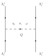
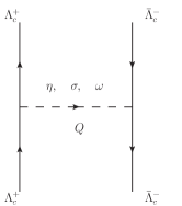
Figure 2: Scattering processes of $\Lambda_{c}\Lambda_{c}\to\Lambda_{c}\Lambda_{c}$ and $\Lambda_{c}\bar{\Lambda}_{c}\to\Lambda_{c}\bar{\Lambda}_{c}$, $Q$s are the transformed four momenta.

Generally speaking, a potential derived from the scattering $T$ matrix consists of the central term, spin-spin interaction term, orbit-spin interaction term and tenser force term, i.e.,

$$V(\bm{r})=V_{C}(r)+V_{SS}(r)\bm{\sigma}_{1}\cdot\bm{\sigma}_{2}+V_{LS}(r)\bm{L}\cdot\bm{S}+V_{T}(r)S_{12}(\hat{\bm{r}}),$$ (21)

where $S_{12}(\hat{\bm{r}})$ is the tensor force operator, $S_{12}(\hat{\bm{r}})=3(\bm{\sigma}_{1}\cdot\hat{\bm{r}})(\bm{\sigma}_{2}\cdot\hat{\bm{r}})-\bm{\sigma}_{1}\cdot\bm{\sigma}_{2}$. The effective potential of a specific channel, for example $\Lambda_{c}\Lambda_{c}\to\Lambda_{c}\Lambda_{c}$ shown in Fig. 2, may contain contributions from the pseudoscalar, vector and scalar meson exchanges. We need work them out one by one and add them. The potentials with the stripped isospin factors from the pseudoscalar, vector and scalar ($\sigma$ here) meson exchange are

$$V^{a}(\bm{r};\alpha,h) = V^{a}_{SS}(r;\alpha,h)\bm{\sigma}_{1}\cdot\bm{\sigma}_{2}+V^{a}_{T}(r;\alpha,h)S_{12}(\hat{\bm{r}}),$$

$$V^{b}(\bm{r};\beta,h) = V^{b}_{C}(r;\beta,h)+V^{b}_{SS}(r;\beta,h)\bm{\sigma}_{1}\cdot\bm{\sigma}_{2}+V^{b}_{LS}(r;\beta,h)\bm{L}\cdot\bm{S}+V^{b}_{T}(r;\beta,h)S_{12}(\hat{\bm{r}}),$$

$$V^{c}(\bm{r};\sigma,h) = V^{c}_{C}(r;\sigma,h)+V^{c}_{LS}(r;\sigma,h)\bm{L}\cdot\bm{S},$$ (22)

where $\alpha=\pi,\eta$, $\beta=\rho,\omega,\phi$ and

$$V^{a}_{SS}(r;\alpha,h) = -\frac{g_{\alpha hh}^{2}}{4\pi}\frac{m_{\alpha}^{3}}{12m_{h}^{2}}H_{1}(\Lambda,m_{\alpha},r),$$

$$V^{a}_{T}(r;\alpha,h) = \frac{g_{\alpha hh}^{2}}{4\pi}\frac{m_{\alpha}^{3}}{12m_{h}^{2}}H_{3}(\Lambda,m_{\alpha},r),$$

$$V^{b}_{C}(r;\beta,h) = \frac{m_{\beta}}{4\pi}\left[g_{\beta hh}^{2}H_{0}(\Lambda,m_{\beta},r)-(g_{\beta hh}^{2}+4g_{\beta hh}f_{\beta hh})\frac{m_{\sigma}^{2}}{8m_{h}^{2}}H_{1}(\Lambda,m_{\beta},r)\right],$$

$$V^{b}_{SS}(r;\beta,h) = -\frac{1}{4\pi}(g_{\beta hh}+f_{\beta hh})^{2}\frac{m_{\beta}^{3}}{6m_{h}^{2}}H_{1}(\Lambda,m_{\beta},r),$$

$$V^{b}_{LS}(r;\beta,h) = -\frac{1}{4\pi}(3g_{\beta hh}^{2}+4g_{\beta hh}f_{\beta hh})\frac{m_{\beta}^{3}}{2m_{h}^{2}}H_{2}(\Lambda,m_{\beta},r),$$

$$V^{b}_{T}(r;\beta,h) = -\frac{1}{4\pi}(g_{\beta hh}+f_{\beta hh})^{2}\frac{m_{\beta}^{3}}{12m_{h}^{2}}H_{3}(\Lambda,m_{\beta},r),$$

$$V^{c}_{C}(r;\sigma,h) = -m_{\sigma}\frac{g_{\sigma hh}^{2}}{4\pi}\left[H_{0}(\Lambda,m_{\sigma},r)+\frac{m_{\sigma}^{2}}{8m_{h}^{2}}H_{1}(\Lambda,m_{\sigma},r)\right],$$

$$V^{c}_{LS}(r;\sigma,h) = -m_{\sigma}\frac{g_{\sigma hh}^{2}}{4\pi}\frac{m_{\sigma}^{2}}{2m_{h}^{2}}H_{2}(\Lambda,m_{\sigma},r).$$ (23)

The definitions of functions $H_{0}$, $H_{1}$, $H_{2}$ and $H_{3}$ are given in the appendix. From Eq. (22), one can see the tensor force terms and spin-spin terms are from the pseudoscalar and vector meson exchanges while the central and obit-spin terms are from the vector and scalar meson exchanges. Finally the effective potential of the state $hh$ is

$$V_{hh}(\bm{r}) = \sum_{\alpha}\mathcal{C}^{a}_{\alpha}V^{a}(\bm{r};\alpha,h)+\sum_{\beta}\mathcal{C}^{b}_{\beta}V^{b}(\bm{r};\beta,h)+\mathcal{C}^{c}_{\sigma}V^{c}(\bm{r};\sigma,h)$$

$$= \left\{\sum_{\beta}\mathcal{C}^{b}_{\beta}V^{b}_{C}(r;\beta,h)+\mathcal{C}^{c}_{\sigma}V^{c}_{C}(r;\sigma,h)\right\}+\left\{\sum_{\alpha}\mathcal{C}^{a}_{\alpha}V^{a}_{SS}(r;\alpha,h)+\sum_{\beta}\mathcal{C}^{b}_{\beta}V^{b}_{SS}(r;\beta,h)\right\}\bm{\sigma}_{1}\cdot\bm{\sigma}_{2}$$

$$+\left\{\sum_{\beta}\mathcal{C}^{b}_{\beta}V^{b}_{LS}(r;\beta,h)+\mathcal{C}^{c}_{\sigma}V^{c}_{LS}(r;\beta,h)\right\}\bm{L}\cdot\bm{S}+\left\{\sum_{\alpha}\mathcal{C}^{a}_{\alpha}V^{a}_{T}(r;\alpha,h)+\sum_{\beta}\mathcal{C}^{b}_{\beta}V^{b}_{T}(r;\beta,h)\right\}S_{12}(\hat{\bm{r}}),$$

where $\mathcal{C}^{a}_{\alpha}$, $\mathcal{C}^{b}_{\beta}$ and $\mathcal{C}^{c}_{\sigma}$ are the isospin factors, which are listed in Table 1.

	$\Lambda_{c}\Lambda_{c}[\bar{\Lambda}_{c}]$	$\Xi_{c}\Xi_{c}[\bar{\Xi}_{c}]$		$\Sigma_{c}\Sigma_{c}[\bar{\Sigma}_{c}]$			$\Xi_{c}^{{}^{\prime}}\Xi_{c}^{{}^{\prime}}[\bar{\Xi}_{c}^{{}^{\prime}}]$		$\Omega_{c}\Omega_{c}[\bar{\Omega}_{c}]$
I	0	0	1	0	1	2	0	1	0
$\mathcal{C}_{\pi}^{a}$				-2[2]	-1[1]	1[-1]	-3[3]	1[-1]
$\mathcal{C}_{\eta}^{a}$				1[1]	1[1]	1[1]	1[1]	1[1]	1[1]
$\mathcal{C}_{\rho}^{b}$		-3[-3]	1[1]	-2[-2]	-1[-1]	1[1]	-3[-3]	1[1]	1[1]
$\mathcal{C}_{\omega}^{b}$	1[-1]	1[-1]	1[-1]	1[-1]	1[-1]	1[-1]	1[-1]	1[-1]
$\mathcal{C}_{\phi}^{b}$		1[-1]	1[-1]				1[-1]	1[-1]	1[-1]
$\mathcal{C}_{\sigma}^{c}$	1[1]	1[1]	1[1]	1[1]	1[1]	1[1]	1[1]	1[1]

Table 1: Isospin factors. The values in brackets for baryonia are derived by the “G-Parity rule”.

Given the effective potential $V_{hh}$, the potential for $h\bar{h}$, $V_{h\bar{h}}$, can be obtained using the “G-Parity rule”, which states that the amplitude (or the effective potential) of the process $A\bar{A}\to A\bar{A}$ with one light meson exchange is related to that of the process $AA\to AA$ by multiplying the latter by a factor $(-)^{I_{G}}$, where $(-)^{I_{G}}$ is the G-Parity of the exchanged light meson IGrule . The expression of $V_{h\bar{h}}$ is the same as Eq. (II.3) but with $V^{a}(\bm{r};\alpha,h)$, $V^{b}(\bm{r};\beta,h)$ and $V^{c}(\bm{r};\sigma,h)$ replaced by $V^{a}(\bm{r};\alpha,\bar{h})$, $V^{b}(\bm{r};\beta,\bar{h})$ and $V^{c}(\bm{r};\sigma,\bar{h})$ respectively.

$$V^{a}(\bm{r};\alpha,\bar{h}) = (-)^{I_{G}[\alpha]}V^{a}(\bm{r};\alpha,h),$$

$$V^{b}(\bm{r};\beta,\bar{h}) = (-)^{I_{G}[\beta]}V^{b}(\bm{r};\beta,h),$$

$$V^{c}(\bm{r};\sigma,\bar{h}) = (-)^{I_{G}[\sigma]}V^{c}(\bm{r};\sigma,h).$$ (25)

For example,

$$V^{a}(\bm{r};\omega,\bar{\Lambda}_{c}) = (-1)V^{a}(\bm{r};\omega,\Lambda_{c}),$$ (26)

since the G-Parity of $\omega$ is negative. In other words, we can still use the right hand side of Eq. (II.3) to calculate $V_{h\bar{h}}$ but with the redefined isospin factors

$$\mathcal{C}^{a}_{\alpha}\to(-)^{I_{G}[\alpha]}\mathcal{C}^{a}_{\alpha},\;\;\mathcal{C}^{b}_{\beta}\to(-)^{I_{G}[\beta]}\mathcal{C}^{b}_{\beta},\;\;\mathcal{C}^{c}_{\sigma}\to(-)^{I_{G}[\sigma]}\mathcal{C}^{c}_{\sigma},$$ (27)

which are listed in Table 1 too.

The treatments of operators $\bm{\sigma}_{1}\cdot\bm{\sigma}_{2}$, $\bm{L}\cdot\bm{S}$ and $S_{12}(\hat{\bm{r}})$ are straightforward. For ${}^{1}S_{0}$,

$$\bm{\sigma}_{1}\cdot\bm{\sigma}_{2}=-3,\;\;\bm{L}\cdot\bm{S}=0,\;\;S_{12}(\hat{\bm{r}})=0,$$ (28)

which lead to single channel Shrödinger equations. But for ${}^{3}S_{1}$, because of mixing with ${}^{3}D_{1}$, the above operators should be represented in the $\left\{|^{3}S_{1}\rangle,|^{3}D_{1}\rangle\right\}$ space, i.e.,

$$\bm{\sigma}_{1}\cdot\bm{\sigma}_{2}=\left(\begin{array}[]{cc}1&0\\ 0&1\end{array}\right),\;\;\bm{L}\cdot\bm{S}=\left(\begin{array}[]{cc}0&0\\ 0&-3\end{array}\right),\;\;S_{12}(\hat{\bm{r}})=\left(\begin{array}[]{cc}0&\sqrt{8}\\ \sqrt{8}&-2\end{array}\right).$$ (35)

These representations lead to the coupled channel Shrödinger equations.

III Coupling Constants

It is difficult to extract the coupling constants in the Lagrangians experimentally. We may estimate them using the well-known nucleon-meson coupling constants as inputs with the help of the quark model. The details of this method are provided in Ref. Riska2001 . The one-boson exchange Lagrangian at the quark level is

$$\mathcal{L}_{q} = g_{\pi qq}\left(\bar{u}i\gamma_{5}u\pi^{0}-\bar{d}i\gamma_{5}d\pi^{0}\right)$$ (36)

$$+g_{\eta qq}\left(\bar{u}i\gamma_{5}u\eta+\bar{d}i\gamma_{5}d\eta-2\bar{s}i\gamma_{5}s\eta\right)$$

$$+g_{\rho qq}\left(\bar{u}\gamma_{\mu}u\rho^{0\mu}-\bar{d}\gamma_{\mu}d\rho^{0\mu}\right)$$

$$+g_{\omega qq}\left(\bar{u}\gamma_{\mu}u\omega^{\mu}+\bar{d}\gamma_{\mu}d\omega^{\mu}\right)+g_{\phi qq}\bar{s}\gamma_{\mu}s\phi^{\mu}$$

$$+g_{\sigma qq}\left(\bar{u}u\sigma+\bar{d}d\sigma+\bar{s}s\sigma\right)+\cdots,$$

where $g_{\pi qq}$, $g_{\eta qq}$, $\ldots$, $g_{\sigma qq}$ are the coupling constants of the light mesons and quarks. The vector meson terms in this Lagrangian do not contain the anomalous magnetic moment part because the constituent quarks are treated as point-like particles. At the hadronic level, for instance, the nucleon-nucleon-meson interaction Lagrangian reads

$$\mathcal{L}_{NN} = g_{\pi NN}\bar{N}i\gamma_{5}\bm{\tau}N\cdot\bm{\pi}+g_{\eta NN}\bar{N}i\gamma_{5}N\eta$$ (37)

$$+g_{\rho NN}\bar{N}\gamma_{\mu}\bm{\tau}N\cdot\bm{\rho}^{\mu}+\frac{f_{\rho NN}}{2m_{N}}\bar{N}\sigma_{\mu\nu}\bm{\tau}N\cdot\partial^{\mu}\bm{\rho}^{\nu}$$

$$+g_{\omega NN}\bar{N}\gamma_{\mu}N\omega^{\mu}+\frac{f_{\omega NN}}{2m_{N}}\bar{N}\sigma_{\mu\nu}N\partial^{\mu}\omega^{\nu}$$

$$+g_{\sigma NN}\bar{N}N\sigma,$$

where $g_{\pi NN}$, $g_{\eta NN}$, $\ldots$, $g_{\sigma NN}$ are the coupling constants. We calculate the matrix elements for a specific process both at quark and hadronic levels and then match them. In this way, we get relations between the two sets of coupling constants,

$$g_{\pi NN}=\frac{5}{3}g_{\pi qq}\frac{m_{N}}{m_{q}},\;\;g_{\eta NN}=g_{\eta qq}\frac{m_{N}}{m_{q}},$$

$$g_{\omega NN}=3g_{\omega qq},\;\;\frac{g_{\omega NN}+f_{\omega NN}}{m_{N}}=\frac{g_{\omega qq}}{m_{q}},$$

$$g_{\rho NN}=g_{\rho qq},\;\;\frac{g_{\rho NN}+f_{\rho NN}}{m_{N}}=\frac{5}{3}\frac{g_{\rho qq}}{m_{q}},$$

$$g_{\sigma NN}=3g_{\sigma qq}.$$ (38)

From these relations, we can see that $g_{\omega NN}$ and $f_{\omega NN}$ are not independent. So are $g_{\rho NN}$ and $f_{\rho NN}$. The constituent quark mass is about one third of the nucleon mass. Thus we have $f_{\omega NN}\approx 0$ and $f_{\rho NN}\approx 4g_{\rho NN}$.

With the same prescription, we can obtain similar relations for heavy charmed baryons which are collected in the appendix. Substituting the coupling constants at the quark level with those from Eq. (38), we have

$$g_{\pi\Xi_{c}\Xi_{c}}=0,\;\;g_{\pi\Sigma_{c}\Sigma_{c}}=\frac{4}{5}g_{\pi NN}\frac{m_{\Sigma_{c}}}{m_{N}},\;\;g_{\pi\Xi_{c}^{\prime}\Xi_{c}^{\prime}}=\frac{2}{5}g_{\pi NN}\frac{m_{\Xi_{c}^{\prime}}}{m_{N}},$$ (39)

$$g_{\eta\Lambda_{c}\Lambda_{c}}=0,\;\;g_{\eta\Xi_{c}\Xi_{c}}=0,\;\;g_{\eta\Sigma_{c}\Sigma_{c}}=\frac{4}{3}g_{\eta NN}\frac{m_{\Sigma_{c}}}{m_{N}},$$

$$g_{\eta\Xi_{c}^{\prime}\Xi_{c}^{\prime}}=-\frac{2}{3}g_{\eta NN}\frac{m_{\Xi_{c}^{\prime}}}{m_{N}},\;\;g_{\eta\Omega_{c}\Omega_{c}}=-\frac{8}{3}g_{\eta NN}\frac{m_{\Omega_{c}}}{m_{N}},$$ (40)

$$g_{\sigma\Lambda_{c}\Lambda_{c}}=\frac{2}{3}g_{\sigma NN},\;\;g_{\sigma\Xi_{c}\Xi_{c}}=\frac{2}{3}g_{\sigma NN},\;\;g_{\sigma\Sigma_{c}\Sigma_{c}}=\frac{2}{3}g_{\sigma NN},$$

$$g_{\sigma\Xi_{c}^{\prime}\Xi_{c}^{\prime}}=\frac{2}{3}g_{\sigma NN},\;\;g_{\sigma\Omega_{c}\Omega_{c}}=\frac{2}{3}g_{\sigma NN},$$ (41)

$$g_{\omega\Lambda_{c}\Lambda_{c}}=\frac{2}{3}g_{\omega NN},\;\;f_{\omega\Lambda_{c}\Lambda_{c}}=-\frac{2}{3}g_{\omega NN},$$

$$g_{\omega\Xi_{c}\Xi_{c}}=\frac{1}{3}g_{\omega NN},\;\;f_{\omega\Xi_{c}\Xi_{c}}=-\frac{1}{3}g_{\omega NN},$$

$$g_{\omega\Sigma_{c}\Sigma_{c}}=\frac{2}{3}g_{\omega NN},\;\;f_{\omega\Sigma_{c}\Sigma_{c}}=\frac{2}{3}g_{\omega NN}\left(2\frac{m_{\Sigma_{c}}}{m_{N}}-1\right),$$

$$g_{\omega\Xi_{c}^{\prime}\Xi_{c}^{\prime}}=\frac{1}{3}g_{\omega NN},\;\;f_{\omega\Xi_{c}^{\prime}\Xi_{c}^{\prime}}=\frac{1}{3}g_{\omega NN}\left(2\frac{m_{\Xi_{c}^{\prime}}}{m_{N}}-1\right),$$ (42)

$$g_{\rho\Xi_{c}\Xi_{c}}=g_{\rho NN},\;\;f_{\rho\Xi_{c}\Xi_{c}}=-\frac{1}{5}\left(g_{\rho NN}+f_{\rho NN}\right),$$

$$g_{\rho\Sigma_{c}\Sigma_{c}}=2g_{\rho NN},\;\;f_{\rho\Sigma_{c}\Sigma_{c}}=\frac{2}{5}\left(g_{\rho NN}+f_{\rho NN}\right)\left(2\frac{m_{\Sigma_{c}}}{m_{N}}-1\right),$$

$$g_{\rho\Xi_{c}^{\prime}\Xi_{c}^{\prime}}=g_{\rho NN},\;\;f_{\rho\Xi_{c}^{\prime}\Xi_{c}^{\prime}}=\frac{1}{5}\left(g_{\rho NN}+f_{\rho NN}\right)\left(2\frac{m_{\Xi_{c}^{\prime}}}{m_{N}}-1\right),$$ (43)

$$g_{\phi\Xi_{c}\Xi_{c}}=\sqrt{2}g_{\rho NN},\;\;f_{\phi\Xi_{c}\Xi_{c}}=-\frac{\sqrt{2}}{5}\left(g_{\rho NN}+f_{\rho NN}\right),$$

$$g_{\phi\Xi_{c}^{\prime}\Xi_{c}^{\prime}}=\sqrt{2}g_{\rho NN},\;\;f_{\phi\Xi_{c}^{\prime}\Xi_{c}^{\prime}}=\frac{\sqrt{2}}{5}\left(g_{\rho NN}+f_{\rho NN}\right)\left(2\frac{m_{\Xi_{c}^{\prime}}}{m_{N}}-1\right),$$

$$g_{\phi\Omega_{c}\Omega_{c}}=2\sqrt{2}g_{\rho NN},\;\;f_{\phi\Omega_{c}\Omega_{c}}=\frac{2\sqrt{2}}{5}(g_{\rho NN}+f_{\rho NN})\left(2\frac{m_{\Omega_{c}}}{m_{N}}-1\right),$$ (44)

where we have used $m_{N}\approx 3m_{q}$. The couplings of $\phi$ and heavy charmed baryons can not be derived directly from the results for nucleons. So in the right hand side of Eq. (44), we use the couplings of $\rho$ and nucleons.

The above formula relate the unknown coupling constants for heavy charmed baryons to $g_{\pi NN}$, $g_{\eta NN}$, etc. which can be determined by fitting to experimental data. We choose the values $g_{\pi NN}=13.07$, $g_{\eta NN}=2.242$, $g_{\sigma NN}=8.46$, $g_{\omega NN}=15.85$, $f_{\omega NN}/g_{\omega NN}=0$, $g_{\rho NN}=3.25$ and $f_{\rho NN}/g_{\rho NN}=6.1$ from Refs. Mach87 ; Mach01 ; Cao2010 as inputs. In Table 2, we list the numerical results of the coupling constants of the heavy charmed baryons and light mesons. One notices that the vector meson couplings for $\Xi_{c}\Xi_{c}$ and $\Lambda_{c}\Lambda_{c}$ have opposite signs. They almost cancel out and do not contribute to the tensor terms for spin-triplets. Thus in the following numerical analysis, we omit the tensor forces of the spin-triplets in the $\Xi_{c}\Xi_{c}$ and $\Lambda_{c}\Lambda_{c}$ systems.

	$\Lambda_{c}\Lambda_{c}$		$\Xi_{c}\Xi_{c}$		$\Sigma_{c}\Sigma_{c}$		$\Xi_{c}^{{}^{\prime}}\Xi_{c}^{{}^{\prime}}$		$\Omega_{c}\Omega_{c}$
$\alpha$	$g_{\alpha\Lambda_{c}\Lambda_{c}}$	$f_{\alpha\Lambda_{c}\Lambda_{c}}$	$g_{\alpha\Xi_{c}\Xi_{c}}$	$f_{\alpha\Xi_{c}\Xi_{c}}$	$g_{\alpha\Sigma_{c}\Sigma_{c}}$	$f_{\alpha\Sigma_{c}\Sigma_{c}}$	$g_{\alpha\Xi_{c}^{{}^{\prime}}\Xi_{c}{{}^{\prime}}}$	$f_{\alpha\Xi_{c}^{{}^{\prime}}\Xi_{c}^{{}^{\prime}}}$	$g_{\alpha\Omega_{c}\Omega_{c}}$	$f_{\alpha\Omega_{c}\Omega_{c}}$
$\pi$			0		$27.36$		$14.36$
$\eta$	$0$		$0$		$7.82$		$-4.10$		$-17.19$
$\sigma$	$5.64$		$5.64$		$5.64$		$5.64$		$5.64$
$\omega$	$10.57$	$-10.57$	$5.28$	$-5.28$	$10.57$	$44.67$	$5.28$	$23.72$
$\rho$			$3.25$	$-4.62$	$6.50$	$39.01$	$3.25$	$20.72$
$\phi$			$4.60$	$-6.53$			$4.60$	$29.30$	$9.19$	$61.94$

Table 2: Numerical results of the coupling constants. The coupling constants with the $\phi$ exchange are deduced from $g_{\rho NN}$.

IV Numerical Results

With the effective potentials and the coupling constants derived in the previous sections, one can calculate the binding energies and root-mean-square (RMS) radii for every possible molecular state numerically. Here we adopt the program FESSDE which is a FORTRAN routine to solve problems of multi-channel coupled ordinary differential equations fessde . Besides the coupling constants in Table 2, we also need heavy charmed baryon masses listed in Table 3 as inputs. The typical value of this cutoff parameter for the deuteron is $1.2\sim 1.5\mathrm{~{}GeV}$ Mach87 . In our case, the cutoff parameter $\Lambda$ is taken in the region $0.80\sim 2.00\mathrm{~{}GeV}$. Such a region is broad and reasonable enough to give us a clear picture of the possibility of the heavy baryon molecules.

baryon	mass(MeV)	baryon	mass(MeV)	meson	mass(MeV)	meson	mass(MeV)
$\Lambda_{c}^{+}$	$2286.5$	$\Sigma_{c}$	$2455$	$\pi^{\pm}$	$139.6$	$\rho$	$775.5$
$\Xi_{c}^{+}$	$2467.8$	$\Xi_{c}^{\prime+}$	$2575.6$	$\pi^{0}$	$135.0$	$\omega$	$782.7$
$\Xi_{c}^{0}$	$2470.9$	$\Xi_{c}^{\prime 0}$	$2577.9$	$\eta$	$547.9$	$\phi$	$1019.5$
$\Omega_{c}^{0}$	$2695.2$			$\sigma$	$600$

Table 3: Masses of heavy baryons and light mesons pdg2010 . We use $m_{\Xi_{c}}=2469.3\mathrm{~{}MeV}$, $m_{\Xi_{c}^{\prime}}=2576.7\mathrm{~{}MeV}$ and $m_{\pi}=138.1\mathrm{~{}MeV}$ as numerical analysis inputs.

IV.1 $\Lambda_{c}\Lambda_{c}$ and $\Xi_{c}\Xi_{c}$ systems

The total effective potential of $\Lambda_{c}\Lambda_{c}$ arises from the $\sigma$ and $\omega$ exchanges. We plot it with $\Lambda=0.9\mathrm{~{}GeV}$ in Fig. 3 (a), from which we can see that the $\omega$ exchange is repulsive while the $\sigma$ exchange is attractive. Because of the cancellation, the total potential is too shallow to bind two $\Lambda_{c}$s. In fact, we fail to find any bound solutions of $\Psi_{\Lambda_{c}\Lambda_{c}}^{[0,1]}$ even if one takes the deepest potential with $\Lambda=0.9\mathrm{~{}GeV}$. In other words, the loosely bound $\Lambda_{c}\Lambda_{c}$ molecular state does not exist, which is the heavy analogue of the famous H dibaryon Aerts:1983hy ; Iwasaki:1987db ; Stotzer:1997vr ; Ahn:1996hw to some extent.

For the $\Lambda_{c}\bar{\Lambda}_{c}$ system as shown in Fig. 3 (b), both $\sigma$ and $\omega$ exchanges are attractive. They enhance each other and lead to a very strong total interaction. From our results listed in Table 4, the binding energies of the $\Lambda_{c}\bar{\Lambda}_{c}$ system could be rather large. For example, when we increase the cutoff to $\Lambda=1.10\mathrm{~{}GeV}$, the corresponding binding energy is $142.19\mathrm{~{}MeV}$. The binding energies and RMS radii of this system are very sensitive to the cutoff, which seems to be a general feature of the systems composed of one hadron and anti-hadron.

(a) $V_{\Lambda_{c}\Lambda_{c}}^{[0,1]}$ with $\Lambda=0.9\mathrm{~{}GeV}$.

(d) $V_{\Xi_{c}\Xi_{c}}^{[0,3]}$ with $\Lambda=1.0\mathrm{~{}GeV}$.

(b) $V_{\Lambda_{c}\bar{\Lambda}_{c}}^{[0,1]}$ with $\Lambda=0.9\mathrm{~{}GeV}$.

(e) $V_{\Xi_{c}\bar{\Xi}_{c}}^{[0,1]}$ with $\Lambda=1.0\mathrm{~{}GeV}$.

(c) $V_{\Xi_{c}\Xi_{c}}^{[1,1]}$ with $\Lambda=1.1\mathrm{~{}GeV}$.

(f) $V_{\Xi_{c}\bar{\Xi}_{c}}^{[1,3]}$ with $\Lambda=1.0\mathrm{~{}GeV}$.

Figure 3: The potentials of $\Psi_{\Lambda_{c}\Lambda_{c}}$, $\Psi_{\Lambda_{c}\bar{\Lambda}_{c}}$, $\Psi_{\Xi_{c}\Xi_{c}}$ and $\Psi_{\Xi_{c}\bar{\Xi}_{c}}$. The spin-triplets have no $S-D$ mixing because of the cancellations of the coupling constants.

	$\Lambda$ (GeV)	E (MeV)	$r_{rms}$(fm)		$\Lambda$ (GeV)	E (MeV)	$r_{rms}$(fm)
					0.89	2.80	2.15
$\Psi_{\Lambda_{c}\Lambda_{c}}^{[0,1]}$		$-$		$\Psi_{\Lambda_{c}\bar{\Lambda}_{c}}^{[0,1(3)]}$	0.90	4.61	1.76
					1.00	49.72	0.74
					1.10	142.19	0.52
	0.95	2.53	2.17		1.01	0.14	5.58
$\Psi_{\Xi_{c}\Xi_{c}}^{[0,3]}$	1.00	7.41	1.41	$\Psi_{\Xi_{c}\Xi_{c}}^{[1,1]}$	1.05	0.29	4.48
	1.10	20.92	0.96		1.10	0.35	4.62
	1.20	36.59	0.78		1.20	0.18	5.40
	0.87	1.48	2.72		0.90	1.24	2.92
$\Psi_{\Xi_{c}\bar{\Xi}_{c}}^{[0,1(3)]}$	0.90	4.12	1.78	$\Psi_{\Xi_{c}\bar{\Xi}_{c}}^{[1,1(3)]}$	1.00	10.33	1.25
	1.00	28.94	0.86		1.10	31.80	0.83
	1.10	82.86	0.60		1.20	66.19	0.64

Table 4: Numerical results of the systems $\Lambda_{c}\Lambda_{c}$, $\Lambda_{c}\bar{\Lambda}_{c}$, $\Xi_{c}\Xi_{c}$ and $\Xi_{c}\bar{\Xi}_{c}$, where “$-$” means no bound state solutions. After neglecting the tensor force terms, the results of spin-triplets are the same as those of spin-singlets.

$\Xi_{c}^{0}$ and $\Xi_{c}^{+}$ contain the $s$ quark and their isospin is $I=1/2$. Besides the $\sigma$ and $\omega$ meson exchanges, the $\phi$ and $\rho$ exchanges also contribute to the potentials for the $\Xi_{c}\Xi_{c}(\bar{\Xi}_{c})$ systems. Figs. 3 (c) and (d) illustrate the total potentials and the contributions from the light meson exchanges for $\Psi_{\Xi_{c}\Xi_{c}}^{[1,1]}$ and $\Psi_{\Xi_{c}\Xi_{c}}^{[0,3]}$. For $\Psi_{\Xi_{c}\Xi_{c}}^{[1,1]}$, the attraction arises from the $\sigma$ exchange. Because of the repulsion provided by the $\phi$, $\rho$ and $\omega$ exchange in short range, the total potential has a shallow well at $r\approx 0.2\mathrm{~{}fm}$. However, the $\phi$ exchange almost does not contribute to the potential of $\Psi_{\Xi_{c}\Xi_{c}}^{[0,3]}$ and the $\rho$ exchange is attractive which cancels the repulsion of the $\sigma$ exchange. The total potential is about two times deeper than the total potential of $\Psi_{\Xi_{c}\Xi_{c}}^{[1,1]}$.

In Table 4, one notices that the binding energy is only hundreds of $\mathrm{~{}keV}$ for $\Psi_{\Xi_{c}\Xi_{c}}^{[1,1]}$ when the cutoff varies from $1.01\mathrm{~{}GeV}$ to $1.20\mathrm{~{}GeV}$. Moreover the RMS radius of this bound state is very large. So the state $\Psi_{\Xi_{c}\Xi_{c}}^{[1,1]}$ is very loosely bound if it really exists. The $\Psi_{\Xi_{c}\Xi_{c}}^{[0,3]}$ bound state may also exist. Its binding energy and RMS radius are $2.53\sim 36.59\mathrm{~{}MeV}$ and $2.17\sim 0.78\mathrm{~{}fm}$ respectively with $\Lambda=0.95\sim 1.20\mathrm{~{}GeV}$.

As for the $\Xi_{c}\bar{\Xi}_{c}$ systems, the potentials are very deep. The contribution from the $\phi$ exchange is negligible too, as shown in Fig. 3 (e) and (f). We find four bound state solutions for these systems: $\Psi_{\Xi_{c}\bar{\Xi}_{c}}^{[0,1]}$, $\Psi_{\Xi_{c}\bar{\Xi}_{c}}^{[0,3]}$, $\Psi_{\Xi_{c}\bar{\Xi}_{c}}^{[1,1]}$ and $\Psi_{\Xi_{c}\bar{\Xi}_{c}}^{[1,3]}$. Among them, the numerical results of $\Psi_{\Xi_{c}\bar{\Xi}_{c}}^{[0,3]}$ and $\Psi_{\Xi\bar{\Xi}_{c}}^{[1,1]}$ are almost the same as those of $\Psi_{\Xi\bar{\Xi}_{c}}^{[0,1]}$ and $\Psi_{\Xi_{c}\bar{\Xi}_{c}}^{[1,3]}$ respectively. The binding energies and the RMS radii of these states are shown in Table 4. We can see that the binding energy of $\Psi_{\Xi_{c}\bar{\Xi}_{c}}^{[0,1]}$ varies from $1.48\mathrm{~{}MeV}$ to $82.86\mathrm{~{}MeV}$ whereas the RMS radius reduces from $2.72\mathrm{~{}fm}$ to $0.60\mathrm{~{}fm}$ when the cutoff is below $1.10\mathrm{~{}GeV}$. The situation of $\Psi_{\Xi_{c}\bar{\Xi}_{c}}^{[1,3]}$ is similar to that of $\Psi_{\Xi_{c}\bar{\Xi}_{c}}^{[0,1]}$ qualitatively. They may exist. But the binding energies appear a little large and the RMS radii too small when one takes $\Lambda$ above $1.10\mathrm{~{}GeV}$.

IV.2 $\Sigma_{c}\Sigma_{c}$, $\Xi^{\prime}_{c}\Xi^{\prime}_{c}$ and $\Omega_{c}\Omega_{c}$ systems

For the $\Sigma_{c}\Sigma_{c}$ system, all the $\pi$, $\eta$, $\sigma$, $\omega$ and $\rho$ exchanges contribute to the total potential. We give the variation of the potentials with $r$ in Figs. 4 (a) and (b). For $\Psi_{\Sigma_{c}\Sigma_{c}}^{[0,1]}$, the potential of the $\omega$ exchange and $\rho$ exchange almost cancel out, and the $\eta$ exchange gives very small contribution. So the total potential of this state mainly comes from the $\pi$ and $\sigma$ exchanges which account for the long and medium range attraction respectively. There may exist a bound state $\Psi_{\Sigma_{c}\Sigma_{c}}^{[0,1]}$, see Table 5.

But for the other spin-singlet, $\Psi_{\Sigma_{c}\Sigma_{c}}^{[2,1]}$, the $\sigma$ exchange provides only as small as $0.2\mathrm{~{}GeV}$ attraction while the $\omega$ and $\rho$ exchanges give strong repulsions in short range $r<0.6\mathrm{~{}fm}$. We have not found any bound solutions for $\Psi_{\Sigma_{c}\Sigma_{c}}^{[2,1]}$ as shown in Table 5. For the spin-triplet state $\Psi_{\Sigma_{c}\Sigma_{c}}^{[1,3]}$, there exist bound state solutions with binding energies between $0.11\mathrm{~{}MeV}$ and $31.35\mathrm{~{}MeV}$ when the cutoff lies between $1.05\mathrm{~{}GeV}$ and $1.80\mathrm{~{}GeV}$. This state is the mixture of ${}^{3}S_{1}$ and ${}^{3}D_{1}$ due to the tensor force in the potential. From Table 5, one can see the $S$ wave percentage is more than $90\%$.

(a) $V_{\Sigma_{c}\Sigma_{c}}^{[0,1]}$ with $\Lambda=1.10\mathrm{~{}GeV}$.

(d) $V_{\Sigma_{c}\bar{\Sigma}_{c}}^{[1,1]}$ with $\Lambda=1.0\mathrm{~{}GeV}$.

(g) $V_{\Xi_{c}^{\prime}\bar{\Xi}_{c}^{\prime}}^{[0,1]}$ with $\Lambda=1.0\mathrm{~{}GeV}$.

(j) $V_{\Omega_{c}\bar{\Omega}_{c}}^{[0,1]}$ with $\Lambda=1.0\mathrm{~{}GeV}$.

(b) $V_{\Sigma_{c}\Sigma_{c}}^{[2,1]}$ with $\Lambda=1.0\mathrm{~{}GeV}$.

(e) $V_{\Sigma_{c}\bar{\Sigma}_{c}}^{[2,1]}$ with $\Lambda=1.0\mathrm{~{}GeV}$.

(h) $V_{\Xi_{c}^{\prime}\bar{\Xi}_{c}^{\prime}}^{[1,1]}$ with $\Lambda=1.0\mathrm{~{}GeV}$.

(c) $V_{\Sigma_{c}\bar{\Sigma}_{c}}^{[0,1]}$ with $\Lambda=1.0\mathrm{~{}GeV}$.

(f) $V_{\Xi_{c}^{\prime}\Xi_{c}^{\prime}}^{[1,1]}$ with $\Lambda=1.70\mathrm{~{}GeV}$.

(i) $V_{\Omega_{c}\Omega_{c}}^{[0,1]}$ with $\Lambda=1.0\mathrm{~{}GeV}$.

Figure 4: Potentials of $\Psi_{\Sigma_{c}\Sigma_{c}}$, $\Psi_{\Sigma_{c}\bar{\Sigma}_{c}}$, $\Psi_{\Xi_{c}^{\prime}\Xi_{c}^{\prime}}$, $\Psi_{\Xi_{c}^{\prime}\bar{\Xi}_{c}^{\prime}}$, $\Psi_{\Omega_{c}\Omega_{c}}$ and $\Psi_{\Omega_{c}\bar{\Omega}_{c}}$.

	$\Lambda$ (GeV)	E (MeV)	$r_{rms}$ (fm)		$\Lambda$ (GeV)	E (MeV)	$r_{rms}$ (fm)	$P_{S}$ :	$P_{D}$ (%)
	1.07	1.80	2.32
	1.08	3.10	1.88
$\Psi_{\Sigma_{c}\Sigma_{c}}^{[0,1]}$	1.10	6.55	1.44	$\Psi_{\Sigma_{c}\Sigma_{c}}^{[0,3]}$		$\times$
	1.20	42.95	0.78
	1.25	75.75	0.65
					1.05	0.11	5.94	98.11	1.89
$\Psi_{\Sigma_{c}\Sigma_{c}}^{[1,1]}$				$\Psi_{\Sigma_{c}\Sigma_{c}}^{[1,3]}$	1.47	2.03	2.48	94.21	5.79
		$\times$			1.50	2.52	2.27	93.79	6.21
					1.80	31.35	0.76	91.41	8.59
$\Psi_{\Sigma_{c}\Sigma_{c}}^{[2,1]}$		$-$		$\Psi_{\Sigma_{c}\Sigma_{c}}^{[2,3]}$		$\times$

Table 5: Numerical results of the $\Sigma_{c}\Sigma_{c}$ system, where the symbol “$\times$” means this state is forbidden and “$-$” means no solutions.

	One Boson Exchange					One Pion Exchange
	$\Lambda$(GeV)	E (MeV)	$r_{rms}$(fm)	$P_{S}$  :	$P_{D}$(%)	$\Lambda$(GeV)	E(MeV)	$r_{rms}$(fm)	$P_{S}$  :	$P_{D}$(%)
	0.97	0.86	3.76
$\Psi_{\Sigma_{c}\bar{\Sigma}_{c}}^{[0,1]}$	0.98	3.03	2.21
	1.00	18.43	1.01					$-$
	1.05	175.56	0.41
	0.93	1.04	3.50	81.20	18.80	0.80	17.54	1.20	82.93	17.07
$\Psi_{\Sigma_{c}\bar{\Sigma}_{c}}^{[0,3]}$	0.94	2.55	2.57	75.27	24.73	0.85	26.33	1.04	81.66	18.34
	1.00	28.16	1.29	58.07	41.93	0.90	37.48	0.92	80.57	19.42
	1.05	78.48	0.99	50.56	49.44	1.05	87.94	0.68	78.03	21.97
	0.93	0.75	3.77
$\Psi_{\Sigma_{c}\bar{\Sigma}_{c}}^{[1,1]}$	0.94	2.54	2.27					$-$
	0.98	32.28	0.80
	1.00	66.97	0.60
	0.80	3.71	1.91	94.73	5.27	0.97	1.04	3.14	93.68	6.32
$\Psi_{\Sigma_{c}\bar{\Sigma}_{c}}^{[1,3]}$	0.81	5.18	1.69	94.38	5.62	1.02	2.51	2.18	91.58	8.42
	0.90	40.35	0.86	90.12	9.88	1.10	6.44	1.51	89.04	10.96
	1.00	143.46	0.62	76.86	23.14	1.30	27.27	0.88	84.89	15.11
	0.80	24.87	0.85			0.75	2.49	1.98
$\Psi_{\Sigma_{c}\bar{\Sigma}_{c}}^{[2,1]}$	0.85	49.30	0.67			0.80	5.95	1.38
	0.90	90.04	0.55			0.90	18.30	0.88
	0.95	149.66	0.46			1.10	72.23	0.51
	0.90	1.44	2.93	96.92	3.08
$\Psi_{\Sigma_{c}\bar{\Sigma}_{c}}^{[2,3]}$	1.00	14.99	1.21	95.43	4.57			$-$
	1.10	41.81	0.86	95.11	4.89
	1.20	77.28	0.71	94.72	5.28

Table 6: Numerical results of the $\Sigma_{c}$-$\bar{\Sigma}_{c}$ system. Results from the OBE and OPE alone are compared.

There exist bound state solutions for all six states of the $\Sigma_{c}\bar{\Sigma}_{c}$ system. The potentials of the three spin-singlets are plotted in Figs.  4 (c)-(e). The attraction that binds the baryonium mainly comes from the $\rho$ and $\omega$ exchanges. These contributions are of relatively short range at region $r<0.6\mathrm{~{}fm}$. One may wonder whether the annihilation of the heavy baryon and anti-baryon might play a role here. Thus the numerical results for $\Sigma_{c}\bar{\Sigma}_{c}$ with strong short-range attractions should be taken with caution. This feature differs from the dibaryon systems greatly.

In Table 6, for comparison, we also present the numerical results with the $\pi$ exchange only. It’s very interesting to investigate whether the long-range one-pion-exchange potential (OPE) alone is strong enough to bind the baryonia and form loosely bound molecular states. There do not exist bound states solutions for $\Psi_{\Sigma_{c}\bar{\Sigma}_{c}}^{[0,1]}$ and $\Psi_{\Sigma_{c}\bar{\Sigma}_{c}}^{[1,1]}$ since the $\pi$ exchange is repulsive. In contrast, the attractions from the $\pi$ exchange are strong enough to form baryonium bound states for $\Psi_{\Sigma_{c}\bar{\Sigma}_{c}}^{[0,3]}$, $\Psi_{\Sigma_{c}\bar{\Sigma}_{c}}^{[1,3]}$ and $\Psi_{\Sigma_{c}\bar{\Sigma}_{c}}^{[2,1]}$. We notice that the $S-D$ mixing effect for the spin-triplets mentioned above is stronger than that for the $\Sigma_{c}\Sigma_{c}$ system.

	$\Lambda$ (GeV)	E (MeV)	$r_{rms}$ (fm)		$\Lambda$ (GeV)	E (MeV)	$r_{rms}$ (fm)	$P_{S}$ :	$P_{D}$ (%)
					0.95	1.22	3.03	97.88	2.12
					0.98	2.44	2.29	97.45	2.55
$\Psi_{\Xi_{c}^{{}^{\prime}}\Xi_{c}^{{}^{\prime}}}^{[0,1]}$		$\times$		$\Psi_{\Xi_{c}^{{}^{\prime}}\Xi_{c}^{{}^{\prime}}}^{[0,3]}$	1.00	3.41	2.01	97.26	2.74
					1.20	15.43	1.16	96.74	3.26
					1.30	21.50	1.03	96.83	3.17
	1.50	0.18	5.52
	1.65	1.24	3.08
$\Psi_{\Xi_{c}^{{}^{\prime}}\Xi_{c}^{{}^{\prime}}}^{[1,1]}$	1.70	1.83	2.64	$\Psi_{\Xi_{c}^{{}^{\prime}}\Xi_{c}^{{}^{\prime}}}^{[1,3]}$			$\times$
	1.80	3.42	2.08
	1.90	5.58	1.74

Table 7: Numerical results of the $\Xi_{c}^{{}^{\prime}}\Xi_{c}^{{}^{\prime}}$ system.

	One Boson Exchanges					One Pion Exchanges
	$\Lambda$ (GeV)	E (MeV)	$r_{rms}$ (fm)	$P_{s}$  :	$P_{D}$(%)	$\Lambda$ (GeV)	E (MeV)	$r_{rms}$ (fm)	$P_{S}$ :	$P_{D}$ (%)
	0.96	0.40	4.57
	0.99	3.22	2.00					$-$
$\Psi_{\Xi_{c}^{{}^{\prime}}\bar{\Xi}_{c}^{{}^{\prime}}}^{[0,1]}$	1.00	5.13	1.65
	1.10	83.53	0.58
	0.80	3.82	1.86	96.33	3.67	1.15	0.77	3.42	94.89	5.11
	0.90	19.40	1.04	94.34	5.66	1.20	1.89	2.35	93.01	6.99
$\Psi_{\Xi_{c}^{{}^{\prime}}\bar{\Xi}_{c}^{{}^{\prime}}}^{[0,3]}$	1.00	59.74	0.74	90.03	9.97	1.40	12.69	1.10	88.10	11.90
	1.05	90.87	0.66	86.20	13.80	1.50	22.91	0.88	86.44	13.56
	0.80	14.13	1.01
$\Psi_{\Xi_{c}^{{}^{\prime}}\bar{\Xi}_{c}^{{}^{\prime}}}^{[1,1]}$	0.90	13.58	1.07					$-$
	1.00	34.00	0.77
	1.10	83.78	0.56
	0.90	0.56	3.99	99.76	0.24
$\Psi_{\Xi_{c}^{{}^{\prime}}\bar{\Xi}_{c}^{{}^{\prime}}}^{[1,3]}$	1.00	7.53	1.41	99.59	0.41			$-$
	1.10	22.97	0.94	99.58	0.42
	1.20	43.80	0.76	99.58	0.42

Table 8: Comparison of the numerical results of the system $\Xi_{c}^{{}^{\prime}}\bar{\Xi}_{c}^{{}^{\prime}}$ in the OBE model and OPE model.

The $\Xi_{c}^{\prime}\Xi_{c}^{\prime}(\bar{\Xi}_{c}^{\prime})$ systems are similar to $\Xi_{c}\Xi_{c}(\bar{\Xi}_{c})$ and the results are listed in Figs. 4 (f)-(h) and Tables 7-8. Among the six bound states, $\Psi_{\Xi_{c}^{\prime}\Xi_{c}^{\prime}}^{[1,1]}$ is the most interesting one. As shown in Fig. 4 (f), the $\eta$ exchange does not contribute to the total potential. The $\pi$ exchange is repulsive. So the dominant contributions are from the $\sigma$, $\omega$, $\rho$ and $\phi$ exchanges, which lead to a deep well around $r=0.6\mathrm{~{}fm}$ and a loosely bound state. When we increase the cutoff from $1.50\mathrm{~{}GeV}$ to $1.90\mathrm{~{}GeV}$, the binding energy of $\Psi_{\Xi_{c}^{\prime}{\Xi}_{c}^{\prime}}^{[1,1]}$ varies from $0.18\mathrm{~{}MeV}$ to $5.58\mathrm{~{}MeV}$, and the RMS radius varies from $5.52$ fm to $1.74\mathrm{~{}fm}$. This implies the existence of this loosely bound state. If we consider the $\pi$ exchange alone, only the $\Psi_{\Xi_{c}^{\prime}\bar{\Xi}_{c}^{\prime}}^{[0,3]}$ state is bound. The percentage of the ${}^{3}S_{1}$ component is more than $86\%$ when $1.15\mathrm{~{}GeV}<\Lambda<1.50\mathrm{~{}GeV}$ as shown in Table 8.

	$\Lambda$ (GeV)	E (MeV)	$r_{rms}$ (fm)		$\Lambda$ (GeV)	E (MeV)	$r_{rms}$ (fm)	$P_{S}$ :	$P_{D}$ (%)
	0.96	1.07	3.04
	0.98	2.67	2.08
$\Psi_{\Omega_{c}\Omega_{c}}^{[0,1]}$	1.00	4.51	1.69	$\Psi_{\Omega_{c}\Omega_{c}}^{[0,3]}$		$\times$
	1.20	5.92	1.59
	1.70	19.88	1.15
	0.90	13.12	1.06		0.80	6.92	1.53	99.64	0.06
	0.97	4.34	1.70		0.88	3.05	1.98	99.96	0.04
$\Psi_{\Omega_{c}\bar{\Omega}_{c}}^{[0,1]}$	1.00	5.01	1.62	$\Psi_{\Omega_{c}\bar{\Omega}_{c}}^{[0,3]}$	1.00	9.77	1.23	99.90	0.10
	1.10	20.96	0.94		1.10	26.22	0.86	99.79	0.21
	1.20	108.50	0.48		1.20	47.23	0.72	99.53	0.47

Table 9: Numerical results of the $\Omega_{c}\Omega_{c}$ and $\Omega_{c}\bar{\Omega}_{c}$ systems.

The $\Omega_{c}\Omega_{c}(\bar{\Omega}_{c})$ case is quite simple. Only the $\eta$, $\sigma$ and $\phi$ exchanges contribute to the total potentials. The shape of the potential of $\Psi_{\Omega_{c}\Omega_{c}}^{[0,1]}$ is similar to that of $\Psi_{\Xi_{c}^{\prime}\Xi_{c}^{\prime}}^{[1,1]}$. The binding energy of this state is very small. For the spin-triplet $\Omega_{c}\bar{\Omega}_{c}$ system, its $S$ wave percentage is more than $99\%$. In other words, the $S-D$ mixing effect is tiny for this system.

We give a brief comparison of our results with those of Refs. Froemel:2004ea ; JuliaDiaz:2004rf in Table 10. In Ref. Froemel:2004ea , Fröemel et al. deduced the potentials of nucleon-hyperon and hyperon-hyperon by scaling the potentials of nucleon-nucleon. With the nucleon-nucleon potentials from different models, they discussed possible molecular states such as $\Xi_{cc}N$, $\Xi_{c}\Xi_{cc}$, $\Sigma_{c}\Sigma_{c}$ etc.. The second column of Table 10 shows the binding energies corresponding different models while the last column is the relevant results of this work. One can see the results of Ref. Froemel:2004ea depend on models while our results are sensitive to the cutoff $\Lambda$.

models	Nijm93	NijmI	NijmII	AV18	AV$8^{\prime}$	AV$6^{\prime}$	AV$4^{\prime}$	AV$X^{\prime}$	AV$2^{\prime}$	AV$1^{\prime}$	This work
$[\Xi_{c}^{{}^{\prime}}\Xi_{c}^{{}^{\prime}}]_{I=0}$	-	*	$71.0$	$457.0$	-	$0.7$	$24.5$	$9.5$	$12.8$	-	$1.22\sim 21.50$
$[\Sigma_{c}\Sigma_{c}]_{I=2}$	$66.6$	-	-	$41.1$	-	-	-	-	-	$0.7$	-
$[\Sigma_{c}\Sigma_{c}]_{I=1}$	-	*	$53.7$	-	-	-	$7.3$	$2.8$	$8.3$	$0.7$	$0.11\sim 31.35$
$[\Sigma_{c}\Sigma_{c}]_{I=0}$	*	*	$285.8$	*	$16.1$	$10.8$	$87.4$	$53.3$	$58.5$	$0.7$	$1.80\sim 75.75$

Table 10: The comparison of the binding energies of $\Xi^{\prime}\Xi^{\prime}$ and $\Sigma_{c}\Sigma_{c}$ systems in this work and those in Ref. Froemel:2004ea . The unit is$\mathrm{~{}MeV}$. “-” means there is no bound state and “*” represents exiting unrealistic deeply bindings ($1\sim 10\mathrm{~{}GeV}$).

V Conclusions

The one boson exchange model is very successful in the description of the deuteron, which may be regarded as a loosely bound molecular system of the neutron and proton. It’s very interesting to extend the same framework to investigate the possible molecular states composed of a pair of heavy baryons. With heavier mass and reduced kinetic energy, such a system is non-relativistic. We expect the OBE framework also works in the study of the heavy dibaryon system.

On the other hand, one should be cautious when extending the OBE framework to study the heavy baryonium system. The difficulty lies in the lack of reliable knowledge of the short-range interaction due to the heavy baryon and anti-baryon annihilation. However, there may exist a loosely bound heavy baryonium state when one turns off the short-range interaction and considers only the long-range one-pion-exchange potential. Such a case is particularly interesting. This long-range OPE attraction may lead to a bump, cusp or some enhancement structure in the heavy baryon and anti-baryon invariant mass spectrum when they are produced in the $e^{+}e-$ annihilation or B decay process etc.

In this work, we have discussed the possible existence of the $\Lambda_{c}\Lambda_{c}(\bar{\Lambda}_{c})$, $\Xi_{c}\Xi_{c}(\bar{\Xi}_{c})$, $\Sigma_{c}\Sigma_{c}(\bar{\Sigma}_{c})$, $\Xi^{\prime}_{c}\Xi^{\prime}_{c}(\bar{\Xi}_{c}^{\prime})$ and $\Omega_{c}\Omega_{c}(\bar{\Omega}_{c})$ molecular states. We consider both the long range contributions from the pseudo-scalar meson exchanges and the short and medium range contributions from the vector and scalar meson exchanges.

Within our formalism, the heavy analogue of the H dibaryon $\Psi_{\Lambda_{c}\Lambda_{c}}^{[0,1]}$ does not exist though its potential is attractive. However, the $\Psi_{\Lambda_{c}\bar{\Lambda}_{c}}^{[0,1]}$ and $\Psi_{\Lambda_{c}\bar{\Lambda}_{c}}^{[0,3]}$ bound states might exist. For the $\Xi_{c}\Xi_{c}$ system, there exists a loosely bound state $\Psi_{\Xi_{c}\Xi_{c}}^{[1,1]}$ with a very small binding energy and a very large RMS radius around $5\mathrm{~{}fm}$. The spin-triplet state $\Psi_{\Xi_{c}\Xi_{c}}^{[0,3]}$ may also exist. Its binding energy and RMS radius vary rapidly with increasing cutoff $\Lambda$. The qualitative properties of $\Psi_{\Xi_{c}\bar{\Xi}_{c}}^{[0,1]}$ and $\Psi_{\Xi_{c}\bar{\Xi}_{c}}^{[1,3]}$ are similar to those of $\Psi_{\Lambda_{c}\bar{\Lambda}_{c}}^{[0,1]}$. They could exist but the binding energies and RMS radii are unfortunately very sensitive to the values of the cutoff parameter.

For the $\Sigma_{c}\Sigma_{c}$, $\Sigma_{c}\bar{\Sigma}_{c}$, $\Xi_{c}^{\prime}\Xi_{c}^{\prime}$, $\Xi_{c}^{\prime}\bar{\Xi}_{c}^{\prime}$, $\Omega_{c}\Omega_{c}$ and $\Omega_{c}\bar{\Omega}_{c}$ systems, the tensor forces lead to the $S-D$ wave mixing. There probably exist the $\Sigma_{c}\Sigma_{c}$ molecules $\Psi_{\Sigma_{c}\Sigma_{c}}^{[0,1]}$ and $\Psi_{\Sigma_{c}\Sigma_{c}}^{[1,3]}$ only. For the $\Sigma_{c}\bar{\Sigma}_{c}$ system, the $\omega$ and $\rho$ exchanges are crucial to form the bound states $\Psi_{\Sigma_{c}\bar{\Sigma}_{c}}^{[0,1]}$, $\Psi_{\Sigma_{c}\bar{\Sigma}_{c}}^{[1,1]}$ and $\Psi_{\Sigma_{c}\bar{\Sigma}_{c}}^{[2,3]}$. If one considers the $\pi$ exchange only for the $\Xi_{c}^{\prime}\bar{\Xi}_{c}^{\prime}$ system, there may exist one bound state $\Psi_{\Xi_{c}^{\prime}\bar{\Xi}_{c}^{\prime}}^{[0,3]}$.

The states $\Psi_{\Xi_{c}\Xi_{c}}^{[0,3]}$ and $\Psi_{\Xi_{c}^{\prime}\Xi_{c}^{\prime}}^{[0,3]}$ are very interesting. They are similar to the deuteron. Especially, $\Psi_{\Xi_{c}\Xi_{c}}^{[0,3]}$ and $\Psi_{\Xi_{c}^{\prime}\Xi_{c}^{\prime}}^{[0,3]}$ have the same quantum numbers as deuteron. For $\Psi_{\Xi_{c}\Xi_{c}}^{[0,3]}$, the $S-D$ mixing is negligible whereas for deuteron such an effect can make the percentage of the $D$ wave up to $4.25\%\sim 6.5\%$ Mach87 ; Rijken ; SprungEtc . The $D$ wave percentage of $\Psi_{\Xi_{c}^{\prime}\Xi_{c}^{\prime}}^{[0,3]}$ is $2.12\%\sim 3.17\%$.

The other two states $\Psi_{\Xi_{c}\Xi_{c}}^{[1,1]}$ and $\Psi_{\Xi_{c}^{\prime}\Xi_{c}^{\prime}}^{[1,1]}$ are very loosely bound $S$ wave states. Remember that the binding energy of deuteron is about $2.22\mathrm{~{}MeV}$ HoukAndLeun with a RMS radius $r_{rms}\approx 1.96\mathrm{~{}fm}$ BerardAndSimon . The binding energy and RMS radius of $\Psi_{\Xi_{c}^{\prime}\Xi_{c}^{\prime}}^{[1,1]}$ is quite close to those of the deuteron. In contrast, the state $\Psi_{\Xi_{c}\Xi_{c}}^{[1,1]}$ is much more loosely bound. Its binding energy is only a tenth of that of deuteron.

However, the binding mechanisms for the deuteron and the above four bound states are very different. For the deuteron, the attraction is from the $\pi$ and vector exchanges. But for these four states, the $\pi$ exchange contribution is very small. Either the $\sigma$ (for $\Xi_{c}\Xi_{c}$) or vector meson (for $\Xi_{c}^{\prime}\Xi_{c}^{\prime}$) exchange provides enough attractions to bind the two heavy baryons.

Although very difficult, it may be possible to produce the charmed dibaryons at RHIC and LHC. Once produced, the states $\Xi_{c}\Xi_{c}$ and $\Xi_{c}^{\prime}\Xi_{c}^{\prime}$ are stable since $\Xi_{c}$ and $\Xi_{c}^{\prime}$ decays either via weak or electromagnetic interaction with a lifetime around $10^{-15}s$ pdg2010 . On the other hand, $\Sigma_{c}$ mainly decays into $\Lambda_{c}^{+}\pi$. However its width is only $2.2\mathrm{~{}MeV}$  pdg2010 . The relatively long lifetime of $\Sigma_{c}$ allows the formation of the molecular states $\Psi_{\Sigma_{c}\Sigma_{c}}^{[0,1]}$ and $\Psi_{\Sigma_{c}\Sigma_{c}}^{[0,1]}$. These states may decay into $\Sigma_{c}\Lambda_{c}^{+}\pi$ or $\Lambda_{c}^{+}\Lambda_{c}^{+}\pi\pi$ if the binding energies are less than $131\mathrm{~{}MeV}$ or $62\mathrm{~{}MeV}$ respectively. Another very interesting decay mode is $\Xi_{cc}N$ with the decay momentum around one hundred MeV. In addition, a baryonium can decay into one charmonium and some light mesons. In most cases, such a decay mode may be kinetically allowed. These decay patterns are characteristic and useful to the future experimental search of these baryonium states.

Up to now, many charmonium-like “XYZ” states have been observed experimentally. Some of them are close to the two charmed meson threshold. Moreover, Belle collaboration observed a near-threshold enhancement in $e^{+}e^{-}\to\Lambda_{c}\bar{\Lambda}_{c}$ ISR process with the mass and width of $m=(4634^{+8}_{-7}(stat.)^{+5}_{-8}(sys.))\mathrm{~{}MeV}/c^{2}$ and $\Gamma_{tot}=(92^{+40}_{-24}(stat.)^{+10}_{-21}(sys.))\mathrm{~{}MeV}$ respectively  Pakhlova:2008vn . BaBar collaboration also studied the correlated leading $\Lambda_{c}\bar{\Lambda}_{c}$ production Aubert:2010yz . Our investigation indicates there does exist strong attraction through the $\sigma$ and $\omega$ exchange in the $\Lambda_{c}\bar{\Lambda}_{c}$ channel, which mimics the correlated two-pion and three-pion exchange to some extent.

Recently, ALICE collaboration observed the production of nuclei and antinuclei in $pp$ collisions at LHC  Collaboration:2011yf . A significant number of light nuclei and antinuclei such as (anti)deuterons, (anti)tritons, (anti)Helium3 and possibly (anti)hypertritons with high statistics of over $350\mathrm{~{}M}$ events were produced. Hopefully the heavy dibaryon and heavy baryon and anti-baryon pair may also be produced at LHC. The heavy baryon and anti-baryon pair may also be studied at other facilities such as PANDA, J-Parc and Super-B factories in the future.

APPENDIX

V.1 The functions $H_{0}$, $H_{1}$, $H_{2}$ and $H_{3}$

The functions $H_{0}$, $H_{1}$, $H_{2}$ and $H_{3}$ are defined as Ding

$$H_{0}(\Lambda,m,r) = \frac{1}{mr}\left(e^{-mr}-e^{-\Lambda r}\right)-\frac{\Lambda^{2}-m^{2}}{2m\Lambda}e^{-\Lambda r},$$

$$H_{1}(\Lambda,m,r) = -\frac{1}{mr}(e^{-mr}-e^{-\Lambda r})+\Lambda\frac{\Lambda^{2}-m^{2}}{2m^{3}}e^{-\Lambda r},$$

$$H_{2}\left(\Lambda,m,r\right) = \left(1+\frac{1}{mr}\right)\frac{e^{-mr}}{m^{2}r^{2}}-\left(1+\frac{1}{\Lambda r}\right)\frac{\Lambda}{m}\frac{e^{-\Lambda r}}{m^{2}r^{2}}-\frac{\Lambda^{2}-m^{2}}{2m^{2}}\frac{e^{-\Lambda r}}{mr},$$

$$H_{3}\left(\Lambda,m,r\right) = \left(1+\frac{3}{mr}+\frac{3}{m^{2}r^{2}}\right)\frac{e^{-mr}}{mr}-\left(1+\frac{3}{\Lambda r}+\frac{3}{\Lambda^{2}r^{2}}\right)\frac{\Lambda^{2}}{m^{2}}\frac{e^{-\Lambda r}}{mr}-\frac{\Lambda^{2}-m^{2}}{2m^{2}}\left(1+\Lambda r\right)\frac{e^{-\Lambda r}}{mr}.$$ (45)

With Fourier transformations we have

$$\frac{1}{m^{2}+\bm{Q}^{2}} \rightarrow \frac{m}{4\pi}H_{0}(\Lambda,m,r),$$

$$\frac{\bm{Q}^{2}}{m^{2}+\bm{Q}^{2}} \rightarrow \frac{m^{3}}{4\pi}H_{1}(\Lambda,m,r),$$

$$\frac{\bm{Q}}{m^{2}+\bm{Q}^{2}} \rightarrow \frac{im^{3}\bm{r}}{4\pi}H_{2}(\Lambda,m,r),$$

$$\frac{Q_{i}Q_{j}}{m^{2}+\bm{Q}^{2}} \rightarrow -\frac{m^{3}}{12\pi}\left\{H_{3}(\Lambda,m,r)\left(3\frac{r_{i}r_{j}}{r^{2}}-\delta_{ij}\right)-H_{1}(\Lambda,m,r)\delta_{ij}\right\}.$$ (46)

V.2 The coupling constants of the heavy baryons and light mesons

In the quark model we have

$$g_{\pi\Xi_{c}\Xi_{c}}=0,\;\;g_{\pi\Sigma_{c}\Sigma_{c}}=\frac{4}{3}g_{\pi qq}\frac{m_{\Sigma_{c}}}{m_{q}},\;\;g_{\pi\Xi_{c}^{\prime}\Xi_{c}^{\prime}}=\frac{2}{3}g_{\pi qq}\frac{m_{\Xi^{\prime}_{c}}}{m_{q}},$$

$$g_{\eta\Lambda_{c}\Lambda_{c}}=0,\;\;g_{\eta\Xi_{c}\Xi_{c}}=0,\;\;g_{\eta\Sigma_{c}\Sigma_{c}}=\frac{4}{3}g_{\eta qq}\frac{m_{\Sigma_{c}}}{m_{q}},$$

$$g_{\eta\Xi_{c}^{\prime}\Xi_{c}^{\prime}}=-\frac{2}{3}g_{\eta qq}\frac{m_{\Xi_{c}^{\prime}}}{m_{q}},\;\;g_{\eta\Omega_{c}\Omega_{c}}=-\frac{8}{3}g_{\eta qq}\frac{m_{\Omega_{c}}}{m_{q}},$$

$$g_{\rho\Xi_{c}\Xi_{c}}=g_{\rho qq},\;\;f_{\rho\Xi_{c}\Xi_{c}}=-g_{\rho qq},$$

$$g_{\rho\Sigma_{c}\Sigma_{c}}=2g_{\rho qq},\;\;f_{\rho\Sigma_{c}\Sigma_{c}}=2g_{\rho qq}\left(\frac{2}{3}\frac{m_{\Sigma_{c}}}{m_{q}}-1\right),$$

$$g_{\rho\Xi_{c}^{\prime}\Xi_{c}^{\prime}}=g_{\rho qq},\;\;f_{\rho\Xi_{c}^{\prime}\Xi_{c}^{\prime}}=g_{\rho qq}\left(\frac{2}{3}\frac{m_{\Xi_{c}^{\prime}}}{m_{q}}-1\right),$$

$$g_{\omega\Lambda_{c}\Lambda_{c}}=2g_{\omega qq},\;\;f_{\omega\Lambda_{c}\Lambda_{c}}=-2g_{\omega qq},\;\;g_{\omega\Xi_{c}\Xi_{c}}=g_{\omega qq},\;\;f_{\omega\Xi_{c}\Xi_{c}}=-g_{\omega qq},$$

$$g_{\omega\Sigma_{c}\Sigma_{c}}=2g_{\omega qq},\;\;f_{\omega\Sigma_{c}\Sigma_{c}}=2g_{\omega qq}\left(\frac{2}{3}\frac{m_{\Sigma_{c}}}{m_{q}}-1\right),$$

$$g_{\omega\Xi_{c}^{\prime}\Xi_{c}^{\prime}}=g_{\omega qq},\;\;f_{\omega\Xi_{c}^{\prime}\Xi_{c}^{\prime}}=g_{\omega qq}\left(\frac{2}{3}\frac{m_{\Xi_{c}^{\prime}}}{m_{q}}-1\right),$$

$$g_{\phi\Xi_{c}\Xi_{c}}=g_{\phi qq},\;\;f_{\phi\Xi_{c}\Xi_{c}}=-g_{\phi qq},$$

$$g_{\phi\Xi_{c}^{\prime}\Xi_{c}^{\prime}}=g_{\phi qq},\;\;f_{\phi\Xi_{c}^{\prime}\Xi_{c}^{\prime}}=g_{\phi qq}\left(\frac{2}{3}\frac{m_{\Xi_{c}^{\prime}}}{m_{q}}-1\right),$$

$$g_{\phi\Omega_{c}\Omega_{c}}=2g_{\phi qq},\;\;f_{\phi\Omega_{c}\Omega_{c}}=2g_{\phi qq}\left(\frac{2}{3}\frac{m_{\Omega_{c}}}{m_{q}}-1\right),$$

$$g_{\sigma\Lambda_{c}\Lambda_{c}}=2g_{\sigma qq},\;\;g_{\sigma\Xi_{c}\Xi_{c}}=2g_{\sigma qq},$$

$$g_{\sigma\Sigma_{c}\Sigma_{c}}=2g_{\sigma qq},\;\;g_{\sigma\Xi_{c}^{\prime}\Xi_{c}^{\prime}}=2g_{\sigma qq},\;\;g_{\sigma\Omega_{c}\Omega_{c}}=2g_{\sigma qq}.$$ (47)

Because nucleons do not interact directly with the $\phi$ meson in the quark model, we can not get $g_{\phi qq}$ in this way. However, using the $SU(3)$ flavor symmetry, we have $g_{\phi qq}=\sqrt{2}g_{\rho qq}$. Since $g_{\rho qq}$ is related to $g_{\rho NN}$, all coupling constants of heavy charmed baryons and $\phi$ can be expressed in terms of $g_{\rho NN}$.

V.3 The dependence of the binding energy on the cutoff

Finally, we plot the variations of the binding energies with the cutoff.

(a)

(b)

(c)

(d)

(e)

(f)

(g)

(h)

(i)

(j)

(k)

(l)

Figure 5: Dependence of the binding energy on the cutoff. In Figs.(f) and (i), only one-pion contributions are included.

References

• (1) S. K. Choi, S. L. Olsen, et al. [Belle Collaboration], Phys. Rev. Lett. 91, 262001 (2003); Phys. Rev. Lett. 94, 182002 (2005); Phys. Rev. Lett. 100, 142001 (2008); X. L. Wang, et al. [Belle Collaboration], Phys. Rev. Lett. 99, 142002 (2007); P. Pakhlov, et al. [Belle Collaboration], Phys. Rev. Lett. 100, 202001 (2008).
• (2) B. Aubert, et al. [BaBar Collaboration], Phys. Rev. Lett. 101, 082001 (2008); Phys. Rev. Lett. 95, 142001 (2005); Phys. Rev. Lett. 98, 212001 (2007).
• (3) D. E. Acosta, T. Affolder, et al. [CDF Collaboration], Phys. Rev. Lett. 93, 072001 (2004).
• (4) V. M. Abazov, et al. [D0 Collaboration], Phys. Rev. Lett. 93, 162002 (2004).
• (5) N. Brambilla et al., Eur. Phys. J.  C 71, 1534 (2011) arXiv:1010.5827 [hep-ph].
• (6) E. S. Swanson, Phys. Rept. 429, 243 (2006).
• (7) A. D. Rujula, H. Georgi and S. L. Glashow, Phys. Rev. Lett. 38, 317 (1977).
• (8) N. A. Tornqvist, Z. Phys. C 61, 525 (1994).
• (9) E. S. Swanson, Phys. Lett. B 588, 189 (2004).
• (10) C. Y. Wong, Phys. Rev. C 69, 055202 (2004).
• (11) F. E. Close and P. R. Page, Phys. Lett. B 578, 119 (2004).
• (12) M. B. Voloshin, Phys. Lett. B 579, 316 (2004).
• (13) C. E. Thomas and F. E. Close, Phys. Rev. D 78, 034007 (2008).
• (14) Y. R. Liu, X. Liu, W. Z. Deng and S. L. Zhu, Eur. Phy. J. C 56 63 (2008); X. Liu, Y. R. Liu, W. Z. Deng and S. L. Zhu, Phys. Rev. D 77 094015 (2008); Phys. Rev. D 77, 034003 (2008).
• (15) X. Liu., Z. G. Luo, Y. R. Liu and S. L. zhu, Eur. Phys. J. C 61, 411 (2009); L. L. Shen, X. L. Chen, et al., Eur. Phys. J.  C 70, 183 (2010); B. Hu, X. L. Chen, et al., Chin. Phys.  C 35, 113 (2011); X. Liu and S. L. Zhu, Phys. Rev. D 80, 017502 (2009); X. Liu, Z. G. Luo and S. L. Zhu, arXiv:1011.1045 [hep-ph].
• (16) J. Ping, H. Pang, F. Wang and T. Goldman, Phys. Rev.  C 65, 044003 (2002) [arXiv:nucl-th/0012011].
• (17) G.  J.  Ding, Phys. Rev. D 80, 034005 (2009); G. J. Ding, J. F. Liu and M. L. Yan, Phys. Rev. D 79, 054005 (2009).
• (18) X. Liu, Eur. Phys. J. C 54, 471 (2008).
• (19) F. Huang and Z. Y. Zhang, Phys. Rev. C 72, 068201 (2005); Y. R. Liu and Z. Y. Zhang, Phys. Rev. C 79, 035206 (2009); Q. B. Li, P. N. Shen, Z. Y. Zhang and Y. W. Yu, Nucl. Phys. A 683, 487 (2001).
• (20) Y. R. Liu and M. Oka, arXiv:1103.4624 [hep-ph].
• (21) Y. D. Chen and C. F. Qiao, arXiv:1102.3487 [hep-ph]
• (22) R. Machleidt, K. Holinde and C. Elster, Phys. Rept. 149, 1 (1987).
• (23) R. Machleidt, Phys. Rev. C 63, 024001 (2001).
• (24) M. M. Nagels, T. A. Rijken and J. D. de Swart, Phys. Rev.  D 12 744 (1975); Phys. Rev. D 15 2547 (1977).
• (25) T. M. Yan, et al. Phys. Rev. D 46, 1148 (1992).
• (26) T. Barnes, N. Black, D. J. Dean and E. S. Swanson, Phys. Rev.  C 60, 045202 (1999) [arXiv:nucl-th/9902068].
• (27) E. Klempt, F. Bradamante, et al. Phys. Rept. 368 (2002)
• (28) D. O. Riska and G. E. Brown, Nucl. Phys. A 679, 577 (2001).
• (29) X. Cao, B. S. Zou and H. S. Xu, Phys. Rev. C 81, 065201 (2010).
• (30) A. G. Abrashkevich, D. G. Abrashkevich, M. S. Kaschiev and I. V. Puzynin, Comput. Phys. Commun. 85 65-81 (1995).
• (31) K. Nakamura, et al. (Particle Data Group), J. Phys. G 37, 075021 (2010).
• (32) A. T. M. Aerts and C. B. Dover, Phys. Rev.  D 28, 450 (1983).
• (33) Y. Iwasaki, T. Yoshie and Y. Tsuboi, Phys. Rev. Lett.  60, 1371 (1988).
• (34) R. W. Stotzer et al. [BNL E836 Collaboration], Phys. Rev. Lett.  78, 3646 (1997).
• (35) J. K. Ahn et al. [E224 Collaboration], Phys. Lett.  B 378 (1996) 53.
• (36) F. Fröemel, B. Juliá-Díaz and D. O. Riska, Nucl. Phys.  A 750, 337 (2005) [arXiv:nucl-th/0410034].
• (37) B. Juliá-Díaz and D. O. Riska, Nucl. Phys.  A 755, 431 (2005) [arXiv:nucl-th/0405061].
• (38) R. de Tourreil, B. Rouben and D. W. L. Sprung, Nucl. Phys. A 242 445 (1975); M. Lacombe et al., Phys. Rev. C 21 861 (1980); R. Blankenbecler and R. Sugar, Phys. Rev. 142 (1966) 1051; R. B. Wiringa, R. A. Smith and T. L. Ainsworth, Phys. Rev. C 29 1207 (1984).
• (39) T. L. Houk, Phys. Rev. C 3 1886 (1971); C. van der Leun and C. Alderliesten, Nucl. Phys. A 380 261 (1982).
• (40) G. G. Simon, Ch. Schmitt and V. H. Walther, Nucl. Phys. A 364 (1981) 285; R. W. Bérard et al., Phys. Lett. B 47 355 (1973).
• (41) G. Pakhlova et al. [Belle Collaboration], Phys. Rev. Lett.  101, 172001 (2008) arXiv:0807.4458 [hep-ex].
• (42) B. Aubert et al. [BABAR Collaboration], Phys. Rev.  D 82, 091102 (2010) arXiv:1006.2216 [hep-ex].
• (43) N. S. f. Collaboration, arXiv:1104.3311 [nucl-ex].