Self-organised criticality in base-pair breathing in DNA with a defect

Abstract

We analyse base-pair breathing in a DNA sequence of 12 base-pairs with a defective base at its centre. We use both all-atom molecular dynamics (MD) simulations and a system of stochastic differential equations (SDE). In both cases, Fourier analysis of the trajectories reveals self-organised critical behaviour in the breathing of base-pairs. The Fourier Transforms (FT) of the interbase distances show power-law behaviour with gradients close to $-1$. The scale-invariant behaviour we have found provides evidence for the view that base-pair breathing corresponds to the nucleation stage of large-scale DNA opening (or ’melting’) and that this process is a (second-order) phase transition. Although the random forces in our SDE system were introduced as white noise, FTs of the displacements exhibit pink noise, as do the displacements in the AMBER/MD simulations.
Keywords: DNA, breathers, self-organised criticality, stochastic differential equations, $1/f$ noise.
PACS 05.10.Gg - Stochastic models in statistical physics and nonlinear dynamics
PACS 89.75.Fb - Self-organization in complex systems,
PACS 05.65.+b - Self-organised criticality
PACS 87.14.gk - DNA
MSC 60G18 Probability theory and stochastic processes: self-similar processes
MSC 37K40 Dynamical systems: Soliton theory, asymptotic behavior of solutions
MSC 92C45 Biology and other natural sciences: Kinetics in biochemical problems

1 Introduction

Much has been written about the process by which double-stranded DNA becomes two separated single strands, see, for example, hennig ; amb . Several authors refer to the melting of DNA as having the form of a phase transition, in which the opening of one or a few base-pairs is akin to nucleation, and the subsequent growth of open ‘bubbles’ is similar to the growth of crystal nucleii. This two-stage process is relatively well understood in the contexts of crystal growth, and aerosol formation, but less so in kinetics of DNA replication. The aim of this paper is to show that the nucleation event – that is the initial opening of bases – exhibits self-similar, or scale-free, critical behaviour, as one would expect at a phase transition. Whilst other studies have analysed bubble growth and the statistics of bubble length, we choose to focus on the temporal statistics. Our model is more detailed, only focusing on 12 base-pairs and the opening of the first base; our model is thus significantly smaller than the bubble growth models of hennig ; amb ; however, our models are more accurate in that the AMBER simulations Amber (Assisted Model Building with Energy Refinement) include the effect of every atom in the DNA and the water molecules in the environment, and our SDE models include an accurate fitting of the nonlinear inter-base potential energy as described in our earlier work Duduiala1 .

According to Watson $\&$ Crick Watson , the structure of a DNA duplex consists of two chains of bases. These bases are of four types: the purines Adenine (A) and Guanine (G) and the pyrimidines Cytosine (C) and Thymine (T). Along the chains, the bases are linked by covalent bonds, while the opposite bases from the two chains pair together by two or three hydrogen bonds forming base-pairs. Only A-T or C-G pairs are possible. Given this information, we use a lattice representation for our DNA sequence, as illustrated in Figure 1. Breathing – the localised separation of complementary bases – takes place on the microsecond timescale in normal DNA, which is beyond the range of all-atom molecular dynamics (MD) packages. The insertion of a defect, that is, replacing a thymine (T) with a difluorotoluene (F) base at the lattice site $n=0$, increases the frequency of breathing due to the weakening of the inter-chain potential. This makes breathing occur on the nanosecond timescale and hence it becomes accessible to MD simulation techniques. Biologically the reason for considering the inclusion of a defect is to study fidelity, and the effects of errors, in DNA replication. The defect F has been considered previously, for example, by Cubero et al. cubero , who considered such a system without any externally imposed twist. It is possible that proteins may locally alter the twist of a DNA helix in order to ease the process of localised melting. Hence, here, we impose a twist on the DNA structure in order to investigate its effect on base-pair breathing.

Figure 1: IIllustration of the mesoscopic model of DNA.

In this paper, we analyse base-pair breathing at a defect in double-stranded DNA parameterised using the molecular dynamics (MD) simulation tool AMBER. We consider a range of helicoidal twist angles from 30^∘ to 40^∘ per base-pair at rest, including the typical twist of 36^∘. In Duduiala1 we derived a coarse-grained model based on stochastic differential equations with one variable for the displacement of each base from its equilibrium position. This model includes explicit random forcing terms, which model the interactions of water molecules with the bases, and the whole model has been parameterised to the all-atom MD simulations derived using AMBER. Developed from the models of WattisLaughton ; Wattis , the incorporation of noise and damping terms enables us to investigate the temporal dynamics of breathing. The model is fitted to AMBER data using a sophisticated maximum likelihood estimation procedure which is described in Duduiala1 and summarised in Section 2.2 here. The associated fluctuation-dissipation relation, the dependence of parameters on angle of twist and form of the inter-base potential are also discussed in Duduiala1 .

The DNA sequence under study consists of 12 base-pairs and we have taken that the DNA sequence is surrounded by a water box. The analysis of the simulations of a DNA molecule obtained using AMBER and our SDE system presented in Duduiala1 revealed that the amplitude of fluctuations is slightly reduced in the SDE model, but the breathing length and frequency are similar. In addition, the derivation of the SDE model requires us to modify the fluctuation-dissipation relation in the reduced, or coarse-grained, mesoscopic models. We also make a distinction between the potential of mean force (the free energy) and the various potential energies in our system. This is supported by an analysis of the importance of the damping term in preserving the system energy (which, in combination with the forcing noise terms gives rise to the entropic component of the free energy) and the way in which the along-chain interactions influence the length of a breathing event. We have also shown in Duduiala1 that breathing events are due not only to inhomogeneities in the inter-strand interactions, but also to a significant change in along-chain interactions and the helical twist of the DNA, which potentially influences the interactions between the DNA molecule and the surrounding solvent.

A more detailed analysis of our simulations presented below reveals an interesting result: rather than a well-defined breathing frequency that depends on the twist angle via the energy barrier between open and closed states of the central basepair, we find that at all angles of twist the DNA exhibits breathing across a wide range of frequencies and the amplitude-frequency relationship exhibits scale-free behaviour. Most previous results in the literature show that the energy is transferred between nonlinear localized modes with particular frequencies and between such modes and phonons, as discussed by Peyrard et al. Peyrard ; PeyrardFarago ; PeyrardLopezJames or as shown by the results of Gaeta et al. Gaeta ; Caldarelli ; Cardoni , for example.

In the rest of this section we review some of the relevant theory and applications involving self-organised systems. In Section 2 we outline the models we use and the simulation techniques. Section 3 contains the results of both approaches, showing the consistency of outcomes. Section 4 concludes the paper with a summary and discussion.

1.1 Self-organisation and criticality

Many dynamical systems evolve to a steady state (or an equilibrium) solution or to a limit cycle. More complicated large-time behaviour includes spatio-temporal chaos which is often characterised by strange attractors in phase space Ruelle . Through the study of cellular automata, Wolfram Wolfram characterised large time behaviour into four classes. He empirically identified the following qualitative classes: spatially homogeneous systems (akin to steady-states), periodic structures (limit cycles), systems with chaotic aperiodic behaviour (chaos) and, most notably, a fourth, that of complicated localised and possibly propagating structures. We claim that this last category is the most appropriate classification for the behaviour which we observe later in this paper, and, more precisely, this behaviour corresponds to self-organised criticality (SOC).

In physics, a critical point specifies the conditions, such as temperature, pressure or composition, at which a phase boundary is not valid anymore. Here, by ‘phase’ we understand a state of a system for which the physical properties of a component are uniform. As one approaches the critical point, the properties of the different phases approach each other. In other words, a critical point refers to a system configuration to which the system evolves without ever approaching a fixed equilibrium state. Mathematically, one can define characteristic sizes of behaviour (lengths or timescales of events) which describe the system. When these sizes become infinite the system is classed as critical, that is, fluctuations occur at all length scales.

Systems having the SOC property present a spatially or temporally scale-invariant behaviour without the need to tune any parameter to a specific value. This ubiquity of scale-free behaviour Zinn in such models shows that complex behaviour can be stable. This contrasts with systems where one would generically expect some stable steady behaviour for a wide range of parameter values, and as a parameter changes, one might observe either a smooth change in the system’s behaviour or a bifurcation to a qualitatively different steady-state or limit cycle, for example. In the special case when the parameter takes on the threshold value between two states, more complex phenomena may be observed. This is a typical form of behaviour around a phase transition. In general, the total number of states is finite and the transitions can be characterised using a cellular automaton structure Chopard .

When analysing a large system, we aim to reduce its complexity to a few degrees of freedom, for which the coupling can be defined in a general manner and hence we obtain some averaged, or coarse-grained, behaviour over ignored quantities and includes corresponding averaged interactions within the system and the surrounding environment. For dynamical systems, such a dimensional reduction can be achieved by the “slaving principle” Haken which leads to the the study of low-dimensional attractors. This is often a straightforward method. For example, “fast modes” at equilibrium can be slaved to a few slowly-evolving modes. However, sometimes a system responds on both fast and slow timescales, even at large times, and we require an alternative theory, such as the idea of self-organised systems, whose behaviour cannot be explained using the slaving principle or other reductions.

Some attracting critical points of dynamical systems can be characterised using the concept of self-organized criticality (SOC), which was first introduced by Bak et al. Bak87 ; Bak88 . Using simple automata, they demonstrated power-law relationships and $1/f$ noise (also known as “flicker noise”) in spatially extended systems, this behaviour illustrates critical phenomena, and underpins more general scale-invariant behaviour and fractals. They studied the dynamics of damped pendula and the slope of sandpiles, determining critical points of the systems. One aspect of self-organised criticality is the separation of timescales: in the most familiar application of sandpiles, grains are continually added on a faster timescale. The gradient of the pile slowly steepens and there are avalanches (large-scale reorganisation of the pile) which take place rapidly but are separated by large time intervals (relative to the timescale at which grains are added to the pile). Bak et al also noted that changing the values of system parameters did not affect the emergence of critical behaviour. Avalanches in a one-dimensional sandpile are also analysed by Chapman et al. (see, for example, Chapman2 ) who showed that the distribution of energy discharges due to internal reorganizations have a power-law form and so demonstrate that the system is self-organized.

In general, for a noisy system the power spectrum has the form $S(f)=cf^{-\beta}$, where $c$ is a constant. The noise present in the system can be classified in three important categories as follows:

• white noise, for $\beta=0$;

• pink noise, for $\beta=1$;

• red noise (also known as Brownian noise), for $\beta=2$.

However, the term “$1/f$ noise” is widely used to refer to any noise with a power spectral density $S(f)\propto f^{-\beta}$, with $0<\beta<2$. For $1/f$ noise that occurs in nature, $\beta$ is usually close to 1.

Although there is no single well-defined class of systems having the SOC property, it is typically observed in complex systems with slowly-driven nonequilibrium behaviour, for which the causes of an event taking place in a system cannot be explained simply through some parameter values. Several studies of SOC show that scale-invariant phenomena can be determined at critical points, but not necessarily at any critical point. There are two important categories of such phenomena: fractals Peng and power laws Newman . Whilst the first category involves geometric shapes, which can be split into parts that are reduced-size copies of the initial shape, the second deals with frequency-dependent quantities and, hence, is relevant in the analysis of some Hamiltonian systems. We note that self-organised systems are always at criticality, but not all critical systems are self-organised.

The range of systems exhibiting critical properties varies from earthquakes Olami ; BakEarth and forest-fires BakFF ; Drossel to biological systems, such as proteins Phillips ; Phillips2 , the brain Werner and even DNA. Selvam Selvam2 , for example, studies the distribution of bases in a human DNA sequence and shows that the C-G base-pair frequency distribution exhibits a universal inverse power-law form. Also, Harris et al. Harris analyse the configurational entropy of a DNA molecule based on the entropy estimation for a Gaussian configuration given by Schlitter schlitter , which helps investigate whether a steady state has been reached during a simulation. They show that the estimate of the entropy $S_{n}$ depends on the number of data points $n$ and this relation is a power law (with exponent between zero and minus one).

2 Modelling DNA

In our system, we also have a separation of timescales: there are rapidly oscillating forcing terms applied to the DNA chain illustrated in Figure 1 (these model the interactions with water molecules and are akin to grains being added to the sandpile) and the occasional larger-scale restructuring of the chain as the base-pairs open or close at the start and end of breathing events (which are akin to avalanches in sandpiles). We now discuss in detail the modelling approaches we adopt.

2.1 All-atom MD modelling using AMBER

As already mentioned, we obtain data from an all atom simulation of DNA using the package AMBER Amber . The DNA sequence analysed contains 12 base-pairs as follows:

C	T	T	T	T	G	F	A	T	C	T	T
G	A	A	A	A	C	A	T	A	G	A	A

This sequence is analysed at a constant temperature of $T=293K$, in the presence of a surrounding water box. The solvent has to be taken into account because it influences the displacement of atoms and through other bonds, affects the hydrogen bonds linking the bases on the DNA strands PeyrardLopez . Even if the breathing events occur on the nanosecond time-scale and the DNA sequence contains only 12 base-pairs, which together with the sugars and phosphate groups represent 763 atoms, the number of degrees of freedom in our system is actually very large (16682) due to the water box. This means most of the time is spent computing information about the solvent, even though this information is not used for our analysis, since we focus only on the DNA bases and their dynamics.

Note that AMBER considers that the normal twist by default is about 32.5^∘. In order to avoid this inconvenience, we have constructed the DNA sequence by considering the degree of twist at rest. The degree of twist is preserved by imposing a harmonic restraint on the atoms at the end bases. More precisely, we have considered a constant energy (of 1 kcal mol^-1 Å^-2) and hence a constant force acting on the end bases, in order to keep the DNA atoms close to their initial positions. Applying this restraint to the end bases allows the A-F pair to breathe and so explore a larger volume of phase space than the other base-pairs.

The force field used during the AMBER simulations is also important. For a DNA molecule, the predefined FF99SB all-atom force field was used. Moreover, AMBER provides several water models for residues with name WAT – the default is TIP3P, which was used in our simulations. After creating the topology and coordinates files using the AMBER packages LEaP and nucgen, we have used SANDER for energy minimization. This process involves a structural relaxation, which is necessary because the coordinates file contains some initial values that do not guarantee a minimum energy configuration, this reduces the possibility of having conflicts or overlapping atoms. In addition to energy minimization, we have also performed a few equilibration and MD simulations in which temperature changes.

Finally, our system is simulated using SANDER. Next, ptraj is used to measure the distance between the A-F base-pair as well as the separations of the other base-pairs and the corresponding velocities. This data is output every 1 ps or 2 fs depending on which simulation study is being performed.

2.2 Stochastic mesoscopic model

In DNA, the rapid external fluctuation events correspond to random collisions of the bases with the water molecules surrounding the biopolymer. These events correspond to perturbations to the variables $y_{n}(t)$, fluctuations in these displacements may propagate along the chain, perturbing neighbouring bases, eventually causing the central base $y_{0}(t)$ to cross a barrier in the potential $E_{0}(y_{0})$, see Figure 2.

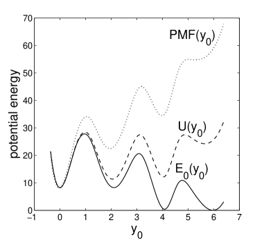
Figure 2: The interchain interaction potential $E_{0}(y_{0})$, the total potential energy $U(y_{0})=E_{0}(y_{0})+\frac{1}{2}\widehat{k}y_{0}^{2}$, and the potential of mean force $PMF(y_{0})=U(y_{0})+\sqrt{k_{B}T}\eta_{0}y_{0}$ used in (4), for a 36^∘ twisted DNA sequence.

A second source of data is the reduced model introduced in Duduiala1 which is based on a system of stochastic ordinary differential equations (SDEs). We start from the deterministic system

$$H = \sum_{n}\left\{\mbox{$\frac{1}{2}$}\dot{u}_{n}^{2}+\mbox{$\frac{1}{2}$}\dot{v}_{n}^{2}+\mbox{$\frac{1}{2}$}\gamma(u_{n}-v_{n})^{2}+\mbox{$\frac{1}{2}$}k(u_{n+1}-u_{n})^{2}+\mbox{$\frac{1}{2}$}k(v_{n+1}-v_{n})^{2}\right\}$$ (1)

$$+\mbox{$\frac{1}{2}$}(\widehat{k}-k)\left[(u_{1}-u_{0})^{2}+(u_{0}-u_{-1})^{2}+(v_{1}-v_{0})^{2}+(v_{0}-v_{-1})^{2}\right]$$

$$+E_{0}(y_{0})-\mbox{$\frac{1}{2}$}\gamma(u_{0}-v_{0})^{2},$$

which is illustrated in Figure 1. Here, $u_{n}(t)$ represent the deviations from equilibrium of the bases on one chain of the DNA, and $v_{n}(t)$ the displacements of the bases on the second chain, with the index $n$ determining the position down each chain ($-6\leq n\leq 5$). Since we are interested in investigating in more detail a system similar to that of Guckian et al. Guckian we place a defect at the centre of the chain, that is, the $u_{0}$ and $v_{0}$ bases correspond to the A-F base-pair. The parameter $k$ describes the stiffness of the backbone down each side of the double-helix structure, whist the parameter $\gamma$ indicates the strength of interaction between a base on one strand and its complement. These forces are assumed to be uniform along the DNA double helix, except at the defect where they are replaced by the parameter $\widehat{k}$ and the nonlinear force $E_{0}^{\prime}(y_{0})$ respectively. To these we add noise and damping terms with coefficients $\epsilon_{*}$ and $\eta_{*}$ respectively. The dependence of all these parameters on the twist angle $\theta$ has been determined in an earlier paper Duduiala1 . We make the transformation $y_{n}=u_{n}-v_{n}$ so as to obtain equations of motion for the distances between base-pairs

$$\!\frac{{\rm d}^{2}\!y_{n}}{{\rm d}t^{2}}\! \!=\! \!k(y_{n+1}\!-\!2y_{n}\!+\!y_{n-1})-\gamma y_{n}-\eta\frac{dy_{n}}{dt}+\epsilon\xi_{n},\quad(|n|>1),$$ (2)

$$\!\;\;\frac{{\rm d}^{2}\!y_{-1}}{{\rm d}t^{2}}\! \!=\! \!\widehat{k}(y_{0}\!-\!y_{-1})-k(y_{-1}\!-\!y_{-2})-\gamma y_{-1}-\eta\frac{{\rm d}y_{-1}}{{\rm d}t}+\epsilon\xi_{-1},$$ (3)

$$\!\frac{{\rm d}^{2}\!y_{0}}{{\rm d}t^{2}}\! \!=\! \!\widehat{k}(y_{1}\!-\!2y_{0}\!+\!y_{-1})-\frac{{\rm d}E_{0}}{{\rm d}y}(y_{0}\!)-\eta_{0}\frac{{\rm d}y_{0}}{{\rm d}t}+\epsilon_{0}\xi_{0},$$ (4)

$$\!\frac{{\rm d}^{2}\!y_{1}}{{\rm d}t^{2}}\! \!=\! \!k(y_{2}\!-\!y_{1})-\widehat{k}(y_{1}\!-\!y_{0})-\gamma y_{1}-\eta\frac{{\rm d}y_{1}}{{\rm d}t}+\epsilon\xi_{1}.$$ (5)

The functions $\xi_{n}(t)$ are white noise forcing terms. The quantities $\gamma$, $k$, $\widehat{k}$, $\epsilon$, $\epsilon_{0}$, $\eta$, $\eta_{0}$ are all fitted using a maximum likelihood estimation procedure, as is the interaction potential $E_{0}(y_{0})$, a full description of this is given in Duduiala1 ; Duduiala4 . A typical example of the multiwelled interaction potential, $E_{0}(y_{0})$ is given in Figure 2. Note that the total potential energy of the central defective base-pair is $U(y_{0})=E_{0}(y_{0})+\frac{1}{2}\widehat{k}y_{0}^{2}$, and the potential of mean force (free energy) is given by $PMF(y_{0})=U(y_{0})+\sqrt{k_{B}T}\eta_{0}y_{0}$, can easily be obtained from simulations by plotting a histogram of binned displacement data.

3 Results

We measure the distance between the two bases (A, F) at the defect over many nanoseconds, that is, we sample $y_{0}(t)$ at specific intervals. Using data from both AMBER and the SDE system we analyse the (discrete) Fourier transforms of $y_{0}(t)$ for a range of twist angles from 30^∘ to 40^∘ per base-pair.

The discrete Fourier transform is taken of the data, in the figures displayed later, we use the notation $DFT(\omega)$ for $\widehat{y}_{0}(\omega)$, and the hypothesis we are testing is that over a wide range of $\omega$,

$$\log\widehat{y}_{0}(\omega)=-\beta\log\omega+\log C.$$ (6)

The highest frequency attainable is $\omega_{{\rm max}}=2\pi/2\Delta t$, whilst the lowest frequency is given by $2\pi/T$ where $T$ is the length of the simulation and $\Delta t$ is the sampling interval. Our initial results are simulations of length approximately $T=10$ ns sampled every $\Delta t=1$ ps (giving $\sim 10^{4}$ data points). We then perform simulations of $T=2$ ns sampled on a much finer scale of $\Delta t=2$ fs (giving $\sim 10^{6}$ data points). These are performed using both AMBER and our SDE system. The SDE system is then subjected to a longer-time simulation of $T=100$ ns, sampled every $\Delta t=1$ ps ($\sim 10^{5}$ data points). This enables a wide range of frequencies to be sampled: for the initial simulations $0.00063<\omega<3.14$ ps^-1 ($-7.4<\log\omega<1.14$), for the more frequently sampled simulations $0.0032<\omega<1600$ ($-5.7<\log\omega<7.4$), and for the long simulations $2\pi\times 10^{-5}<\omega<3.14$ ($-9.7<\log\omega<1.14$).

Other frequencies which might be of relevance in interpreting the results are the upper and lower limits of the phonon band (which we refer to as $\omega_{{\rm opt}}$ and $\omega_{{\rm ac}}$ respectively), and the frequency of the defect mode. Assuming that the defect mode can be approximated by $\ddot{y}_{0}=-E_{0}^{\prime\prime}(0)y_{0}$ we find $E_{0}^{\prime\prime}(0)=14$ and $\omega_{{\rm def}}=3.7$, hence $\log\omega_{{\rm def}}=1.3$. Since $120<\gamma<165$ and $160<\gamma+4k<210$, we have $\omega_{{\rm ac}}=11$ and $\omega_{{\rm opt}}=14.5$, implying $\log\omega_{{\rm ac}}=2.4$ and $\log\omega_{{\rm opt}}=2.7$. These all lie well above the range of frequencies that we shall be interested in below.

3.1 Initial results

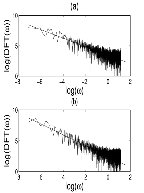
Figure 3: Discrete Fourier transforms (power spectra) of $y_{0}(t)$ plotted against $\omega$ on a log-log scale. Data sampled every 1 ps for 10 ns from a simulation of a 38^∘ twisted DNA sequence from (a) AMBER, and (b) the SDE system (2)–(5).

In Figure 3, we present the log-log plot of the discrete Fourier transform (DFT) against the frequency $\omega$, for $2^{13}$ data points, that is, $y_{0}(t)$ sampled every 1 ps for 8 ns, for a 38^∘ overtwisted DNA sequence. This Figure shows a straight line fit over several orders of magnitude of $\omega$ ($-7<\log_{e}\omega<-1$), with gradients of 0.7–0.9 which are close to $-1$. Similar results are obtained for a 34^∘ twisted DNA sequence, for example, as can be seen in Figure 4. These results suggests that there are breathing events of, and separated by, arbitrarily large times. Thus, if a DNA strand was successively observed for increasingly long intervals of time, there would always be breathing events of duration comparable to the total observation time. The gradients of the $\log_{e}$DFT($\omega$) against $\log_{e}\omega$ lines for the full range of twist angles tested are summarised in Table 1 and suggest the presence of generalised $1/f$ noise in our data (that is, $1/f^{\beta}$ with $0<\beta<2$).

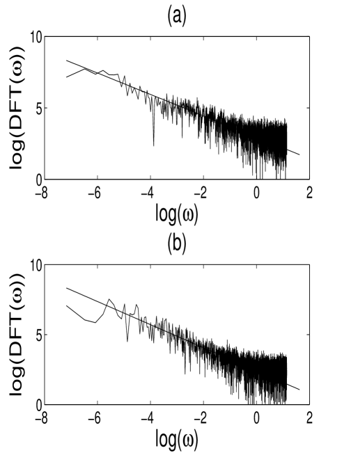
Figure 4: Discrete Fourier transforms (power spectra) of $y_{0}(t)$ plotted against $\omega$ on a log-log scale. Data sampled every 1 ps for 10 ns from a simulation of a 34^∘ twisted DNA sequence from (a) AMBER, and (b) the SDE system (2)–(5).

Angle	$\beta_{AMBER}$	$\;\;\beta_{SDE}\;\;$
30∘	0.725	0.750
32∘	0.700	0.725
33∘	0.725	0.775
34∘	0.750	0.825
35∘	0.750	0.775
36∘	0.775	0.825
38∘	0.700	0.875
40∘	0.700	0.700

Table 1: The gradient $\beta$ of the log-log representation of $DFT(y_{0})$ against $\omega$, from $\sim 10$ ns of data, sampled every 1 ps obtained from the AMBER and SDE models.

Initially our aim was to identify the dominant frequencies of breathers at the defect through the interchain distances. The asymptotic results of Wattis initially appear to suggest that breathers are time-periodic modes with well-defined frequencies; however, that theory actually predicts a one-parameter family of “in-phase” breather modes with frequencies occupying the full range of values from the bottom of the phonon band down to arbitrarily small frequencies (as well as a one-parameter family of “out of phase” breathers with frequencies above the top of the phonon band). Since the part of the frequency range that we are interested in here is the small-$\omega$ limit, it is the former, in-phase, family that concerns us here. We assume that a combination of the stochastic forcing noise and nonlinear interactions of phonons with the breathers which changes their frequency over time and may even sporadically create and destroy the breather modes.

3.2 More refined results

By decreasing the sampling interval ($\Delta t$), we expect to obtain more accurate results; the cost being the increase in data storage requirements. Analysing data sampled every 2 fs for 2.1 ns (more precisely, $2^{20}$ or $10^{6}$ data points), we obtain qualitatively similar results, as can be seen in the results presented in Figure 5, which shows the Fourier power spectra for a DNA helix twisted to 34^∘.

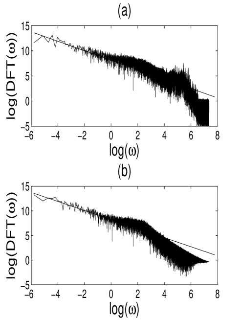
Figure 5: Log-log plots of the discrete Fourier transforms (power spectrum) from more refined samplings of $y_{0}(t)$, specifically, data was sampled every 2 fs for 2.1 ns. Results for a 34^∘ undertwisted DNA sequence from (a) AMBER and (b) the SDE system (2)–(5).

As with the results shown in Section 3.1, the full range of twist angles from 30^∘ to 40^∘ have been simulated and analysed the results are summarised in Table 2. These results, with the reduced sampling interval, suggest that the average value of $\beta$ for such AMBER simulations increases to $0.93$, which is much closer to unity than the values obtained when the sampling interval is $\Delta t=1$ps (Table 1). Analysing a similar data set from the SDE model with more frequent sampling shows a similar increase in $\beta$, from an average of $0.79$ when $\Delta t=1$ps (Table 1) to $\Delta t=0.91$ (Table 2). These results again confirm that our reduced mesoscopic model accurately reproduces the self-organised DNA behaviour observed in the all-atom AMBER simulation. This observed increase in $\beta$ suggests that we might reasonably expect $\beta\rightarrow 1$ as $\Delta t\rightarrow 0$ in both the AMBER and the SDE simulations.

Angle	$\beta_{AMBER}$	$\;\;\beta_{SDE}\;\;$
30∘	0.920	0.900
32∘	0.920	0.895
33∘	0.900	0.910
34∘	0.940	0.920
35∘	0.930	0.900
36∘	0.930	0.910
38∘	0.940	0.940
40∘	0.950	0.905

Table 2: The $\beta$ exponents derived from more refined sampling of $y_{0}(t)$, specifically every 2 fs for 2.1 ns. The $\beta$-exponent is the gradient of the log-log representation of $DFT(y_{0})$ against $\omega$, from AMBER and SDE simulations (compare with Table 1).

At higher values of $\omega$, both AMBER and SDE simulations show changes in behaviour. Firstly, in both cases, the line broadens as more points are plotted at higher values of $\log\omega$ and these display a greater variation; see the ranges $-1<\log\omega<2$ in Figures 3 and 4 and $-1<\log\omega<6$ in Figure 5. Note that the same ranges apply to both AMBER simulations and SDE simulations. Secondly, at larger $\omega$, there is a more significant reduction in the discrete Fourier transform, for the AMBER simulation this occurs from $\omega=2$ upwards, following by a more abrupt decrease around $\omega=6.5$ in Figure 5(a); whereas, in the SDE simulation, Figure 5(b), the spectrum has a simpler form with a more rapid linear decrease with a larger gradient beyond $\omega=2.5$.

3.3 Long-time results

We have analysed a longer simulation of 100 ns, sampling $y_{0}(t)$ every $\Delta t=$ 1 ps using just the SDE system; such a long simulation is beyond the scope of AMBER on currently available computing facilities. This length of simulation allows lower breathing frequencies to be sampled, as shown in Figures 6 and 7. Here we observe the same self-organised behaviour as in earlier graphs, although with some deviation from the straight line at particularly small frequencies, namely those in the range $-9<\log\omega<-7$.

For example, from the $2^{16}(\sim 10^{5})$ data points in the simulation of a 30^∘ undertwisted DNA sequence illustrated in Figure 6, we find $\beta=0.725$. This value is similar to that found in the shorter simulation of 10 ns sampled every 1 ps, where we found $\beta=0.750$; the value of $0.725$ is identical to the value obtained from the shorter AMBER simulation; both these values are reported in Table 1.

For the 38^∘ overtwisted DNA molecule the long-time SDE simulation gives $\beta=0.775$, which lies between the value of $\beta=0.875$ from the shorter SDE simulation and $\beta=0.700$ from the shorter AMBER simulation. Thus for both twist angles, the long-time SDE simulation gives exponents closer to the AMBER results than the shorter SDE simulations.

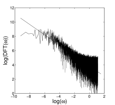
Figure 6: Log-log plot of the discrete Fourier transform (power spectrum) of $y_{0}(t)$ from a long-time (100 ns) SDE simulation for a 30^∘ twisted DNA sequence, $y_{0}(t)$ data sampled every 1 ps.

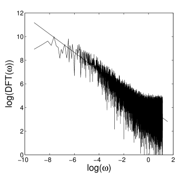
Figure 7: Log-log plot of the discrete Fourier transform (power spectrum) of $y_{0}(t)$ from a long-time (100 ns) SDE simulation for a 38^∘ twisted DNA sequence, $y_{0}(t)$ data sampled every 1 ps.

3.4 Bases away from the defect

Finally we have analysed the motion of the base-pairs adjacent and further away from the defect in the AMBER and SDE systems, in both cases using the example of a 38^∘ overtwisted DNA helix. For example, Figure 8 illustrates the power spectrum of the second-neighbour base-pair $y_{2}{t}$, sampled every 1 ps over a simulation of length 10ns. Although the decay with increasing frequency ($\omega$) is not as clear as in Figures 3, 4, 5, 6, or 7, it is still possible to fit a straight line through the points. For the AMBER and SDE simulations respectively, the gradients of these lines are 0.225 and 0.210 respectively.

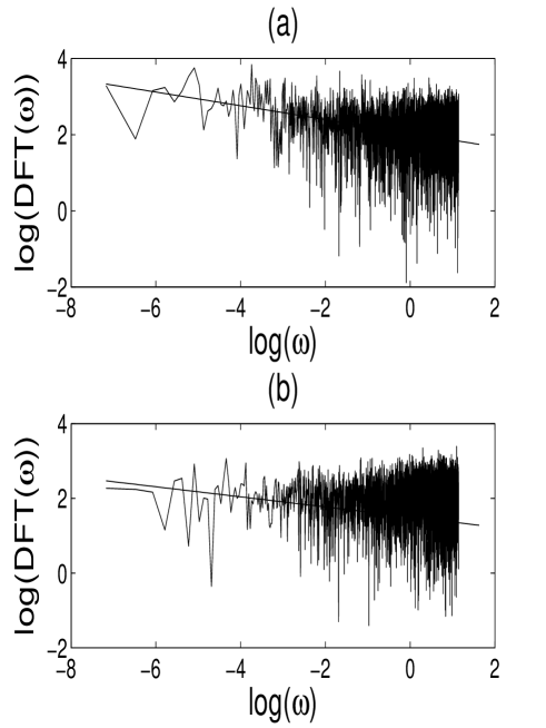
Figure 8: Discrete Fourier transforms (power spectra) of $y_{2}(t)$ plotted against $\omega$ on a log-log scale. Data sampled every 1 ps for 10 ns from a simulation of a 38^∘ twisted DNA sequence from (a) AMBER, and (b) the SDE system (2)–(5).

This procedure has been repeated for the first neighbour base-pair, $y_{1}(t)$, and more distant base-pairs, $y_{3}(t)$, $y_{4}(t)$, and the corresponding gradients of the best fit lines of the log-log plots have been calculated. Assuming that the FTs have power-law forms, these gradients, which correspond to the exponents, $\beta$, are given in Table 3. From the data in this Table we observe that $\beta$ decreases as one moves away from the defect site. This behaviour is due to the reduced influence of the breathing pair on the neighbouring base-pairs. We observe a drop from $\beta\approx 1$ at the defect ($n=0$) to just under one quarter at the nearest neighbour ($n=1$) in both SDE and AMBER.

Base-pair	$\beta_{AMBER}$	$\;\;\beta_{SDE}\;\;$
$y_{1}(t)$	0.225	0.210
$y_{2}(t)$	0.180	0.135
$y_{3}(t)$	0.180	0.130
$y_{4}(t)$	0.180	0.130

Table 3: The gradient $\beta$ of the log-DFT function, from AMBER and SDE data sampled every 1 ps for 10 ns.

Base-pair	$\beta_{AMBER}$	$\;\;\beta_{SDE}\;\;$
$y_{1}(t)$	0.450	0.445
$y_{2}(t)$	0.425	0.205
$y_{3}(t)$	0.410	0.180
$y_{4}(t)$	0.390	0.155

Table 4: The gradient $\beta$ of the log-DFT function, from AMBER and SDE data sampled every 2 fs for 2 ns.

The analysis of $y_{0}(t)$ showed that the exponent $\beta$ increased from $0.7-0.8$ to $0.90-0.95$ when the sampling frequency was decreased from 1ps to 2 fs, suggesting convergence to $\beta=1$ in the limit of small sampling frequency. Hence, we attempt to find more accurate values for the $\beta$-exponent for the neighbouring bases by decreasing the sampling timestep from 1 ps to 2 fs (as we reduce the simulation length from 10ns to 2ns). We obtain the gradients given in Table 4. Summarising, we find values just under one half at the nearest neighbour ($n=1$) in both SDE and AMBER. For $y_{2}$, in AMBER, there is then a further slow decay of ${\cal O}(0.01)$ per base-pair; whereas in SDE there is a more significant drop to 0.2 for $y_{2}$ and then a slow decrease of ${\cal O}(0.01)$ per base-pair. We observe once again that these later results with a decreased sampling timestep of $\Delta t=2$ fs increases the measured values of $\beta$. Hence, we recommend that the even with spatially coarse-grained models of DNA, kinetic characteristics should be analysed using as small a timestep as possible, even as small as 2 fs (as used in AMBER) in order to obtain correct results and conclusions.

This extra decrease in the SDE system may be due to the reduced number of degrees of freedom (only one per base-pair in the SDE), whereas in AMBER there are ${\cal O}(10^{2})$ degrees of freedom per base-pair (the bases having 15 atoms moving in 3D space, in addition to the phosphate backbone). Whilst all base-pairs receive energy in the form of white noise forcing (in the SDE system) and in the form of random collisions with water molecules (AMBER), this energy is used and dissipated differently in the defective base from its neighbours. At the defect, there is a change in temporal behaviour, since white input noise ($\xi_{0}$) is converted to pink output ($y_{0}$) giving $\beta\approx 1$, whereas in the neighbouring bases, the output noise ($y_{n}$) remains significantly closer to white, that is $\beta$ is significantly smaller.

4 Conclusions

In summary, we have simulated a sequence of 12 base-pairs of DNA using two different models for a variety of times up to 100ns. We have analysed the displacement between the defective base-pair near the centre of the chain. Fourier transforms of the distance trajectory taken from both the AMBER and the mesoscopic stochastic differential equation simulations exhibit scale-free, or critical, behaviour for all twist angles in the range 30^∘-40^∘ per base-pair. From (6), we have $\widehat{y}_{0}(\omega)=C\omega^{-\beta}$ across a considerable range of frequencies, $\omega$. Furthermore, we find that $\beta=1$ for all twist angles. Although we have imposed white noise forcing in the system (2)–(5), the noise observed in the output $y_{0}(t)$ is pink ($\beta\approx 1$, Figure 3). This shows that our SDE system preserves the SOC properties of DNA observed in the fully deterministic all-atom AMBER simulations.

It is suspected that proteins which interact with DNA overtwisting or undertwisting the structure in order to ease the release of bases out from the structure. The fact that $\beta=1$ for all twist angles appears to suggest that such a strategy will not change the base-pair breathing. However, the constant $C$ in the formula $\widehat{y}_{0}(\omega)=C\omega^{-\beta}$ will depend on twist angle, and mean that the fraction of time spent in the breathing state is less for the more stable angles $35^{\circ}-36^{\circ}$ and more for the overtwisted or undertwisted DNA structures (i.e those in the ranges $38^{\circ}-40^{\circ}$ and $30^{\circ}-34^{\circ}$ respectively).

What is surprising about our results is that the critical behaviour is not specific to any one twist angle but occurs at all angles. One might expect that, at normal twist angles of 35^∘–36^∘, stable behaviour would be observed, with breathing events having some short characteristic timescale; at smaller and larger twist angles, a critical point would be found, where the DNA exhibited scale-invariant breathing, and that at even more extreme twist angles, the open state would be stable. However, this is not the case at all, instead, we find $1/f$ behaviour at all twist angles. Since the emergence of this critical behaviour is not affected by the variation of the twist angle of the system parameters values, or by the careful tuning of other parameters, we describe this as self-organised criticality.

The scale-free nature of the kinetics of breathing events at all twist angles described herein is strongly reminiscent of the behaviour of fluctuations in systems at criticality. Thus, it appears that without any tuning of the interaction parameters of the DNA strand, it is at a critical point where open bubbles spontaneously nucleate, hence we apply the term ‘self-organized criticality’. Figures 3 and 7 suggest that there is an upper frequency (around $\log_{e}\omega=-1$), above which the amplitude of base-pair separation modes is small but ceases to decay any further, due to the effect of noise in the system. This cutoff is not due to the start of the phonon band (which occupies the range $\sqrt{\gamma}<\omega<\sqrt{\gamma+4k}$), and which corresponds to a relatively narrow range of velocities around $11<\omega<14$ (precise values depend on the twist angle).

We observe some artifacts of the phonon band in the region of $\log\omega$ being between two and three and the defect mode near $\log\omega=1$, in that there is a shoulder in the power spectrum in Figure 5 where the trace is slightly larger than expected; however, no behaviour should be expected to persist over all scales, and the figures show good agreement with scale-free kinetic behaviour (straight-line) over the considerably large range of $-6<\log\omega<1$.

One might think that the defect site is the cause of the SOC breathing behaviour. However, replacing the thymine (T) base with a difluorotoluene (F) base lowers the barrier between the closed and open states. The replacement does not affect the DNA structure or other behaviour, as discussed in several papers, for example, Guckian . Lowering the energy barrier allows breathing to occur at lower energies, and so occur with a higher frequency, on a timescale accessible to MD simulations (on the nanosecond timescale as opposed to the microsecond scale for a normal DNA sequence). There is no reason to suppose that a change in the frequency of events should cause a more significant change in qualitative behaviour. Hence, we speculate that in pure DNA, with no defect, but with multiwelled potentials between all corresponding base-pairs, curves such as that seen in Figure 3, will be repeated but that the crossover frequency (from $\omega$-independent noise to breathing with amplitude proportional to $1/\omega$) will be shifted to much lower frequencies, namely the microsecond scale, which is beyond current MD simulations. Here we only have a double-well potential at the defect, the other inter-base interactions are all governed by harmonic potentials, in reality, all inter-base interactions are double-welled, this will allow an open base-pair to be the nucleus for a bubble of several consecutive open base-pairs to form, as the along-chain interactions would then ease the opening of neighbouring base-pairs.

Acknowledgments

CID was funded by the EU as part of MMBNOTT – an Early Training Research Programme in Mathematical Medicine and Biology.

References

- (1) D. Hennig - Formation and propagation of oscillating bubbles in DNA initiated by structural distortions, Eur. Phys. J. B 37, 391–397, (2004).
- (2) T. Ambjörnsson, S.K. Banik, M.A. Lomholt & R. Metzler - Master equation approach to DNA breathing in heteropolymer DNA, Phys Rev E 75, 021908, (2007).
- (3) D.A. Case, T.A. Darden, T.E. Cheatham, III, C.L. Simmerling, J. Wang, R.E. Duke, R. Luo, K.M. Merz, D.A. Pearlman, M. Crowley, R.C. Walker, W. Zhang, B. Wang, S. Hayik, A. Roitberg, G. Seabra, K.F. Wong, F. Paesani, X. Wu, S. Brozell, V. Tsui, H. Gohlke, L. Yang, C. Tan, J. Mongan, V. Hornak, G. Cui, P. Beroza, D.H. Mathews, C. Schafmeister, W.S. Ross, & P.A. Kollman, AMBER 9, University of California, San Francisco (2006).
- (4) C.I. Duduială, J.A.D. Wattis, I.L. Dryden & C.A. Laughton - Nonlinear breathing modes at a defect site in DNA, Phys Rev E, 80, 061906, (2009).
- (5) J.A.D. Wattis, S.A. Harris, C.R. Grindon & C.A. Laughton - Dynamic model of base pair breathing in a DNA chain with a defect, Phys Rev E, 63, 061903, (2001).
- (6) J.A.D. Wattis - Nonlinear breathing modes due to a defect in a DNA chain, Phil Trans Roy Soc Lond A, 362, 1461–1477, (2004).
- (7) J.D. Watson & F.H.C. Crick - Molecular structure of nucleic acids, Nature 171, 737 (1953).
- (8) E. Cubero, E.C. Sherer, F.J. Luque, M. Orozco & C.A. Laughton - Observation of spontaneous base pair breathing events in the molecular dynamics simulation of a difluorotoluene-containing DNA oligonucleotide, J. Am. Chem. Soc. 121, 8653–8654, (1999).
- (9) M. Peyrard & A.R. Bishop - Statistical mechanics of a nonlinear model for DNA denaturation, Phys Rev, 62, 2755-2758 (1989).
- (10) M. Peyrard & J. Farago - Nonlinear localization in thermalized lattices: Application to DNA, Physica A 288, 199-217 (2000).
- (11) M. Peyrard, S.C. López & G. James - Modelling DNA at the mesoscale: a challenge for nonlinear science?, Nonlinearity 21, T91-T100 (2008).
- (12) G. Gaeta & L. Venier - Solitary waves in twist-opening models of DNA dynamics, Phys Rev E 78, 011901 (2008).
- (13) G. Caldarelli, R. Frondoni, A. Gabrielli1, M. Montuori1, R. Retzlaff & C. Ricotta - Percolation in real wildfires, Europhys Lett 56, 510-516 (2001).
- (14) M. Cadoni, R. De Leo & G. Gaeta - A composite model for DNA torsion dynamics, Phys Rev E 75 021919 (2007).
- (15) D. Ruelle - Small random perturbations of dynamical systems and the definition of attractors, Commun Math Phys 82, 137-151 (1981).
- (16) S. Wolfram - Cellular automata as model of complexity, Nature 311, 419 (1984).
- (17) H. Haken - Cooperative phenomena in systems far from thermal equilibrium and in nonphysical systems, Rev Mod Phys 47, 67-121 (1975).
- (18) J. Zinn-Justin - Quantum Field Theory and Critical Phenomena, Oxford University Press (2002).
- (19) B. Chopard & M. Droz - Cellular Automata Modeling of Physical Systems, Cambridge University Press (1998).
- (20) G. Peng & D. Tian - The fractal nature of a fracture surface, J Phys A: Math Gen 23, 3257-3261 (1990).
- (21) M.E.J. Newman - Power laws, Pareto distributions and Zipf’s law, Contemporary Physics 46(5), 323-351 (2005).
- (22) P. Bak, C. Tang & K. Wiesenfeld - Self-organized criticality: An explanation of the 1/f noise, Phys Rev Lett 59, 381–384, (1987).
- (23) P. Bak, C. Tang & K. Wiesenfeld - Self-organized criticality, Phys Rev A 38, 364–374, (1988).
- (24) S.C. Chapman - Inverse cascade avalanche model with limit cycle exhibiting period doubling, intermittency, and self-similarity, Phys Rev E 62, 1905–1911, (2000).
- (25) Z. Olami, H.J.S. Feder & K. Christensen- Self-organised criticality in a continuous, nonconservative cellular automaton modelling earthquakes, Phys Rev Lett 68, 1244–1247, (1992).
- (26) P. Bak, K. Christensen, L. Danon & T. Scanlon - Unified scaling law for earthquakes, Phys Rev Lett 88, 178501, (2002).
- (27) P. Bak, K. Chen & C. Tang - A forest-fire model and some thoughts on turbulence, Phys Lett A 147, 297–300, (1990).
- (28) B. Drossel & F. Schwabl - Self-organized critical forest-fire model, Phys Rev Lett 69, 1629–1632, (1992).
- (29) J.C. Phillips - Scaling and self-organized criticality in proteins I, Proc Natl Acad Sci 106(9), 3107–3112, (2009).
- (30) J.C. Phillips - Scaling and self-organized criticality in proteins II, Proc Natl Acad Sci 106(9), 3113–3118, (2009).
- (31) G. Werner - Metastability, criticality and phase transitions in brain and its models, Biosystems 90, 496–508, (2007).
- (32) A.M. Selvam - Universal spectrum for DNA base C-G frequency distribution in Human chromosomes 1 to 24, arXiv:physics/0701079 (2007).
- (33) S.A. Harris, E. Gavathiotis, M.S. Searle, M. Orozco & C.A. Laughton - Cooperativity in drug-DNA recognition: a molecular dynamics study, J Am Chem Soc 123, 12658–12663, (2001).
- (34) J. Schlitter - Estimation of absolute and relative entropies of macromolecules using the covariance matrix, Chem. Phys. Lett. 215, 617–621, (1993).
- (35) C.I. Duduială - Stochastic Nonlinear Models of DNA Breathing at a Defect, http://etheses.nottingham.ac.uk/, PhD Thesis, University of Nottingham, (2009).
- (36) M. Peyrard, S. C. López, D. Angelov - Fluctuations in the DNA double helix, Eur Phys J Special Topics 147, 173-189 (2007).
- (37) K.M. Guckian, T.R. Krugh & E.T. Kool - Solution structure of a DNA duplex containing a replicable difluorotoluene-adenine pair, Nature Structural Biology 5, 954–959, (1998).