Discussion of: A statistical analysis of multiple temperature proxies: Are reconstructions of surface temperatures over the last
1000 years reliable?

10.1214/10-AOAS398

Discussion on A statistical analysis of multiple temperature proxies: Are reconstructions of surface temperatures over the last 1000 years reliable? by B. B. McShane and A. J. Wyner

and

t1This research was supported in part by NSF Grant DMS-07-43459. t2This research was supported in part by the Institute of Education Sciences, U.S. Department of Education Grant R305D100017.

1 Introduction

It is a pleasure to have the opportunity to read and comment on McShane and Wyner’s paper, “A statistical analysis of multiple temperature proxies.” This is a must read for every statistician who has an interest in the climate change debate that continues to be a source of intense public policy discussions. The authors are to be congratulated for writing a clear and accessible article that helps decipher the statistics behind the scientific claims related to the paleoclimatological side of the issue.

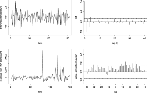
Figure 1: Upper panel shows time series plot and ACF of differenced temperature series; lower panel shows residuals from time series fit to the first component in the PCA decomposition of the proxies and the corresponding cross-correlation function with the temperature series. The code for producing these graphs can be found in Davis and Liu (2011).

We will focus our discussion on some of the points dealing with the time series modeling aspects. The main objectives presented in this paper are strategies for selecting and evaluating predictive models of average yearly temperature that include nearly 1200 proxies. For the sake of this discussion, we will concentrate on the response consisting of the CRU Nothern Hemisphere annual mean land temperature (upper-left panel of Figure 5 in the paper) from 1850 to 1999. Roughly, one can discern three or possibly four segments in this time series: the first from 1850 to 1920 with nearly constant mean, the second from 1921 to 1970 with a mean that is increasing slightly, and the third from 1971 to 1999 with a sharply increasing mean. This is roughly consistent with the three segments found by the segmentation program AutoPARM, developed by Davis, Lee anf Rodriguez-Yam (2006). If we let $Y_{1},\ldots,Y_{150}$ denote the temperature data during these 150 years, 1850–1999, the differenced series $\nabla Y_{t}=Y_{t}-Y_{t-1}$ and its autocorrelation function (ACF) are plotted in the upper-left and right panels of Figure 1. The differenced series looks stationary and the ACF has a spike of $-$0.5 at lag 1, has small values for lags 2 and 3 and is essentially 0 for lags greater than 4. This ACF has the signature of a classical moving average time series with a unit root. Such an ACF suggests a model that takes the form

$$Y_{t}=X_{t}+Z_{t},$$

where $\{Z_{t}\}$ is IID with mean 0 and variance $\sigma^{2}$ and the signal $X_{t}$ is slowly moving with $\nabla X_{t}=X_{t}-X_{t-1}$ being small and having little temporal dependence. If one views the signal as a proxy for the regression function consisting of linear combinations of proxies, then there is just not much signal present. This is consistent with McShane and Wyner’s observation that “the temperature signal in the proxy record is surprisingly weak.” So in this case, the simple diagnostic of looking at the ACF of the differenced series has revealed a great deal about the structure of the time series. In particular, it more than likely excludes a random walk model for the data.

In building forecast models, the inclusion of proxies or covariates is not always straightforward. Often, and as illustrated in this paper, a pure time series model can be as effective for forecasting future (or past) values as one that includes a range of covariates. In fact, a particular covariate that is independent of the response, but is able to mimic the dependence structure of the response, can lead to spurious results. Given the nature of the temperature time series, and the seemingly poor performance of the optimal linear models under consideration, one wonders if a more sophisticated time series modeling approach that incorporates nonlinear effects in a few well-chosen covariates would be more effective. To illustrate this point, consider only one covariate corresponding to the component with largest variance in the PCA decomposition based on the 1209 covariates in the period 1851–2000. The residuals $\hat{u}_{t}$ in fitting an ARMA model to this data are displayed in the lower-left panel of Figure 1. Notice the two large outliers occurring at times 1930 and 1970 as well as a possible increase in variance during the last 30 years. As rightly pointed out in the McShane–Wyner paper, in looking for significant cross-correlation in a time series, one of the component series should first be whitened. In this case we whitened the PCA factor and computed the cross-correlation between $\hat{u}_{t}$ with the temperature time series $Y_{t}$. The sample correlations between $Y_{t+h}$ and $\hat{u}_{t}$, for lags $h=-40,\ldots,40$, are displayed in the lower-right panel of Figure 1 together with 95% confidence bounds based on the two series being uncorrelated. At lag zero, there is virtually no correlation between the two series. The largest and significant correlations occur at lags $h=14$ and 28, suggesting a period of around 14 years in the dependence between the two series. So in building a regression model of the form used in Section 5.1 of the McShane–Wyner paper, it may make more sense to lag the PCA component by $-14$ instead of using the contemporaneous component. This brings up the entire issue of time synchronization with the proxies, which seems to have been ignored entirely in this paper’s discussion. It is puzzling that we find a lagged effect in which the covariate leads (happens before) the response. Based on physical considerations, it would seem that proxies should follow rather than lead temperature. It is easy to construct scenarios in which a proxy provides no forecasting information when only included contemporaneously, but has a strong predictive effect when lagged. In any case, lagged effects with the covariates should be more fully explored and included as potential covariates in the model.

It would be worth exploring potential connections between outliers in the covariate series corresponding with other features in the temperature series. For example, the PCA residual time series graphed in the lower-left panel of Figure 1 displays outliers at years 1931 and 1968 that are relatively close to the times at which we noticed a structural break in the actual temperature series. Each of these years corresponds to a change in slope of the linear trend. While we are not suggesting such a simplistic model for the temperature series, this example suggests a range of models that may carry more predictive skill. We think the interesting comparison would be between the regression models with covariates chosen from a large set of proxies versus a transfer-style model [see, e.g., Brockwell and Davis (2002)] that uses a handful of strategically selected covariates. Transfer functions are also amenable for capturing intervention effects and can serve as a starting point for capturing nonlinear effects between the response and proxies.

Certainly, the paleoclimatological reconstruction problem offers a difficult modeling challenge to climatologists and statisticians alike. It will be fascinating to see the fruits of these efforts in years to come.

R-code for computing the graphs displayed in Figure 1
[doi]10.1214/10-AOAS398CSUPP [url]http://lib.stat.cmu.edu/aoas/398C/supplementC.txt .txt This code can be used to reproduce the graphs displayed in Figure 1.

References

- Brockwell and Davis (2002) {bbook}[mr] \bauthor\bsnmBrockwell, \bfnmPeter J.\binitsP. J. and \bauthor\bsnmDavis, \bfnmRichard A.\binitsR. A. (\byear2002). \btitleIntroduction to Time Series and Forecasting, \bedition2nd ed. \bpublisherSpringer, \baddressNew York. \biddoi=10.1007/b97391, mr=1894099 \endbibitem
- Davis, Lee and Rodriguez-Yam (2006) {barticle}[mr] \bauthor\bsnmDavis, \bfnmRichard A.\binitsR. A., \bauthor\bsnmLee, \bfnmThomas C. M.\binitsT. C. M. and \bauthor\bsnmRodriguez-Yam, \bfnmGabriel A.\binitsG. A. (\byear2006). \btitleStructural break estimation for nonstationary time series models. \bjournalJ. Amer. Statist. Assoc. \bvolume101 \bpages223–239. \biddoi=10.1198/016214505000000745, mr=2268041 \endbibitem
- Davis and Liu (2011) {bmisc}[auto:STB—2010-11-18—09:18:59] \bauthor\bsnmDavis, \bfnmR. A.\binitsR. A. and \bauthor\bsnmLiu, \bfnmJ.\binitsJ. (\byear2011). \bhowpublishedSupplement to “Discussion of: A statistical analysis of multiple temperature proxies: Are reconstructions of surface temperatures over the last 1000 years reliable?” DOI: 10.1214/10-AOAS398CSUPP. \endbibitem