Discussion of: A statistical analysis of multiple temperature proxies: Are reconstructions of surface temperatures over the last
1000 years reliable?

10.1214/10-AOAS398

Discussion on A statistical analysis of multiple temperature proxies: Are reconstructions of surface temperatures over the last 1000 years reliable? by B. B. McShane and A. J. Wyner T1Lamont–Doherty Earth Observatory contribution number 7438.

t1Supported by grants from the NSF (ATM-0902436), NOAA (NA07OAR4310060), and NASA (NNX09AF44G).

McShane and Wyner (2011) (hereinafter MW2011) demonstrated that in many cases a comprehensive data set of $p=1138$ proxies [Mann et al. (2008)] did not predict Northern Hemisphere (NH) mean temperatures significantly better than random numbers. This fact is not very surprising in itself: the unsupervised selection of good predictors from a set of $p\gg n$ proxies of varying sensitivities might be too challenging a task for any statistical method ($p/n_{c}\approx 10$; only $n_{c}=119$ out of total $n=149$ years were used for calibration in MW2011 cross-validated reconstructions). However, some types of noise systematically outperformed the real proxies (see two bottom panels of MW2011, Figure 10). This finding begs further investigation: what do these random numbers have that real proxies do not?

To investigate this question, the present analysis uses ridge regression [RR, Hoerl and Kennard (1970)] instead of the Lasso [Tibshirani (1996)]. The regression model used by MW2011 with Lasso and here with RR is

$$y=X\beta+\beta_{0}\mathbh{1}_{n}+\varepsilon,$$

where $y$ is a column vector of $n$ observations (annual NH temperatures), $\varepsilon$ is random error, $X$ is a known $n\times p$ matrix of predictors (climate proxies). A vector of regression coefficients $\beta$ and an intercept constant $\beta_{0}$ are to be determined. A column $n$-vector $\mathbh{1}_{n}$ has all components equal one. Proxy records are standardized before use; in cross-validation experiments standardization is repeated for each calibration period.

Let $w$ be a column $n_{c}$-vector such that $w^{T}\mathbh{1}_{n_{c}}=1$. Define matrix-valued functions $\mathcal{W}[w]=I-\mathbh{1}_{n_{c}}w^{T}$ and $\mathcal{R}[S,\lambda,w]=S_{vc}(S_{cc}+\lambda I)^{-1}\mathcal{W}[w]+\mathbh{1}_{n_{v}}w^{T},$ where $S$ is a positive semidefinite $n\times n$ matrix, $\lambda>0$ is the ridge parameter found as a minimizer of the generalized cross-validation function [GCV, Golub et al. (1979)], matrix (or vector) subscripts $c$ or $v$ hereinafter indicate submatrices corresponding to the calibration or validation periods, respectively. The RR reconstruction $\hat{y}_{v}$ of temperatures in the validation period (a “holdout block” of $n_{v}=30$ consecutive years) is a linear transformation: $\hat{y}_{v}=\mathcal{R}[S_{p},\lambda,e]y_{c}$, where $S_{p}=\widetilde{X}\widetilde{X}^{T}/p$, $\widetilde{X}$ is the standardized version of $X$, and $e={n}_{c}^{-1}\mathbh{1}_{n_{c}}$.

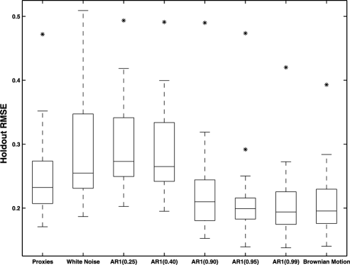
Figure 1: Cross-validated RMSE on 120 30-year holdout blocks for the RR reconstructions from real climate proxies and from the random noise (one realization for each noise experiment); cf. MW2011, Figure 9.

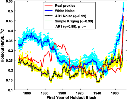
Figure 2: Holdout RMSE for RR reconstructions as a function of time for real proxies (red) and two $100$-member ensemble means: white noise (blue) and $\operatorname{AR}(1)$ noise with $\varphi=0.99$ (black). The probability limit $(p\rightarrow\infty)$ for the latter is shown by magenta dashes. Holdout RMSE for simple kriging of the NH mean temperature index using an exponential semivariogram [Le and Zidek (2006)] $\gamma(\tau)=\lambda_{\min}+1-\exp[\tau\ln\varphi]$ with the GCV-selected nugget $\lambda_{\min}=\ell(\Phi,0)$ and long decorrelation scale $-1/\ln(\varphi)=99.5$ years ($\tau$ is time in years) is shown by the green line. Individual ensemble members are shown by magenta and yellow dots, respectively.

Using these formulas, the RR version of the MW2011 cross-validation tests were performed for real proxies and for some noise types. Results are shown in Figure 1. The cross-validated root mean square error (RMSE) of the RR reconstructions are smaller than Lasso values (cf. MW2011, Figure 9), but the relative performance in different experiments appears consistent between RR and Lasso. As in the Lasso case, noise with high temporal persistence, that is, simulated by the Brownian motion or by the first-order autoregressive process $\operatorname{AR}(1)$ with a parameter $\varphi\geq 0.9$, outperformed proxies. Figure 2 illustrates the time dependence of the holdout error for the real-proxy, white-noise, and $\varphi=0.99$ AR(1) cases. There is a general similarity between these and the corresponding curves in Figure 10 by MW2011.

Note that a traditional approach to hypothesis testing would evaluate an RMSE corresponding to a regression of temperature data ($y$) on real proxies ($X$) in the context of the RMSE probability distribution induced by the assumed distribution of $y$ under the hypothesized condition (e.g., $\beta=0$). However, MW2011 evaluate the RMSE of real proxies in the context of the RMSE distribution induced by random values in $X$, not $y$. Such an approach to testing a null hypothesis would be appropriate for an inverse relationship, that is, $X=y\beta^{T}+\mathbh{1}_{n}\beta_{0}^{T}+\varepsilon$. When used with a direct regression model here, however, it results in the RMSE distribution with a surprising feature: when $p\rightarrow\infty$, RMSE values for individual realizations of the noise matrix $X$ converge in probability to a constant.

This convergence occurs because the columns $x$ of $X$ in the noise experiments are i.i.d. from the noise distribution; AR(1) with $\varphi=0.99$ is considered here: $x\sim\mathcal{N}(0,\Phi),\Phi=(\varphi^{|i-j|})$. The columns of $\widetilde{X}$ are i.i.d. too, hence the random matrix $S_{p}=\widetilde{X}\widetilde{X}^{T}/p$ is an average of $p$ i.i.d. variates $\tilde{x}\tilde{x}^{T}$. Expectation $\Psi=\mathbf{E}\tilde{x}\tilde{x}^{T}$ exists; its elements are computed as expectations of ratios and first inverse moments of quadratic forms in normal variables [Jones (1986, 1987)]. The weak law of large numbers applies, so $S_{p}\stackrel{{\scriptstyle P}}{{\rightarrow}}\Psi$. Since the GCV function depends on $S$ and $w$ as well as on $\lambda$, its minimizing $\lambda$ will depend on these parameters too: $\lambda_{\min}=\ell[S,w]$. Here GCV is assumed well-behaved, so that $\ell$ is a single-valued function, continuous at $(\Psi,e)$. From the definition of $\mathcal{R}$, $\mathcal{B}[S,e]\equiv\mathcal{R}[S,\ell[S,e],e]$ will also be continuous at $S=\Psi$, thus $S_{p}\stackrel{{\scriptstyle P}}{{\rightarrow}}\Psi$ implies $\hat{y}_{v}=\mathcal{B}[S_{p},e]y_{c}\stackrel{{\scriptstyle P}}{{\rightarrow}}\mathcal{B}[\Psi,e]y_{c}$.

When $p$ is finite but large, like $p=1138$, reconstructions based on individual realizations of a noise matrix $X$ are dominated by their constant components, especially when $\varphi\approx 1$: note the small scatter of RMSE values in the ensemble of AR(1) with $\varphi=0.99$ (yellow dots in Figure 2). The probability limit $\hat{y}_{v}=\mathcal{B}[\Psi,e]y_{c}$ yields RMSE values (magenta dash in Figure 2) that are very close ($1.3{\cdot}10^{-3\,\circ}$C RMS difference) to the ensemble mean RMSE (black curve in Figure 2). To interpret this non-random reconstruction, consider its simpler analogue, using neither proxy standardization nor a regression intercept ($\beta_{0}$). Then, if the assumptions on the GCV function change accordingly, $\hat{y}_{v}\stackrel{{\scriptstyle P}}{{\rightarrow}}\mathcal{B}[\Phi,0]y_{c}=\Phi_{vc}[\Phi_{cc}+\ell(\Phi,0)I]^{-1}y_{c}$, that is, a prediction of $y_{v}$ from $y_{c}$ by “simple kriging” [Stein (1999, page 8)], which in atmospheric sciences is called objective analysis or optimal interpolation [Gandin (1963)]. The RMSE corresponding to this solution is shown in Figure 2 (green line): it is quite close to the ensemble mean RMSE for AR(1) noise with $\varphi=0.99$ (RMS difference is $5.4{\cdot}10^{-3\,\circ}$C). The solution $\mathcal{B}[\Psi,e]y_{c}$, to which the noise reconstructions without simplifications converge as $p\rightarrow\infty$, is more difficult to interpret. Still, it has a structure of an objective analysis solution and gives results that are similar to simple kriging: the RMS difference between the two reconstructions over all holdout blocks is $7.7{\cdot}10^{-3\,\circ}$C.

Due to the large value of $p$ in the MW2011 experiments, their tests with the noise in place of proxies essentially reconstruct holdout temperatures by a kriging-like procedure in the temporal dimension. The covariance for this reconstruction procedure is set by the temporal autocovariance of the noise. Long decorrelation scales ($\varphi\geq 0.95$) gave very good results, implying that long-range correlation structures carry useful information about predictand time series that is not supplied by proxies. By using such a noise for their null hypothesis, MW2011 make one skillful model (multivariate linear regression on proxies) compete against another (statistical interpolation in time) and conclude that a loser is useless. Such an inference does not seem justified.

Modern analysis systems do not throw away observations simply because they are less skillful than other information sources: instead, they combine information. MW2011 experiments have shown that their multivariate regressions on the proxy data would benefit from additional constraints on the temporal variability of the target time series, for example, with an AR model. After proxies are combined with such a model, a test for a significance of their contributions to the common product could be performed.

References

- Gandin (1963) {bbook}[auto:STB—2010-11-18—09:18:59] \bauthor\bsnmGandin, \bfnmL. S.\binitsL. S. (\byear1963). \btitleObjective Analysis of Meteorological Fields. \bnoteGidrometeorologicheskoye Izdatel’stvo, Leningrad. Translated from Russian, Israeli Program for Scientific Translations. Jerusalem, 1965. \endbibitem
- Golub, Heath and Wahba (1979) {barticle}[mr] \bauthor\bsnmGolub, \bfnmGene H.\binitsG. H., \bauthor\bsnmHeath, \bfnmMichael\binitsM. and \bauthor\bsnmWahba, \bfnmGrace\binitsG. (\byear1979). \btitleGeneralized cross-validation as a method for choosing a good ridge parameter. \bjournalTechnometrics \bvolume21 \bpages215–223. \bidmr=0533250 \endbibitem
- Hoerl and Kennard (1970) {barticle}[auto:STB—2010-11-18—09:18:59] \bauthor\bsnmHoerl, \bfnmA. E.\binitsA. E. and \bauthor\bsnmKennard, \bfnmR. W.\binitsR. W. (\byear1970). \btitleRidge regression: Biased estimation for non-orthogonal problems. \bjournalTechnometrics \bvolume12 \bpages55–67. \endbibitem
- Jones (1986) {barticle}[mr] \bauthor\bsnmJones, \bfnmM. C.\binitsM. C. (\byear1986). \btitleExpressions for inverse moments of positive quadratic forms in normal variables. \bjournalAustral. J. Statist. \bvolume28 \bpages242–250. \bidmr=0860469 \endbibitem
- Jones (1987) {barticle}[mr] \bauthor\bsnmJones, \bfnmM. C.\binitsM. C. (\byear1987). \btitleOn moments of ratios of quadratic forms in normal variables. \bjournalStatist. Probab. Lett. \bvolume6 \bpages129–136. \biddoi=10.1016/0167-7152(87)90086-1, mr=0907273 \endbibitem
- Le and Zidek (2006) {bbook}[mr] \bauthor\bsnmLe, \bfnmNhu D.\binitsN. D. and \bauthor\bsnmZidek, \bfnmJames V.\binitsJ. V. (\byear2006). \btitleStatistical Analysis of Environmental Space–Time Processes. \bpublisherSpringer, \baddressNew York. \bidmr=2223933 \endbibitem
- Mann et al. (2008) {barticle}[pbm] \bauthor\bsnmMann, \bfnmMichael E.\binitsM. E., \bauthor\bsnmZhang, \bfnmZhihua\binitsZ., \bauthor\bsnmHughes, \bfnmMalcolm K.\binitsM. K., \bauthor\bsnmBradley, \bfnmRaymond S.\binitsR. S., \bauthor\bsnmMiller, \bfnmSonya K.\binitsS. K., \bauthor\bsnmRutherford, \bfnmScott\binitsS. and \bauthor\bsnmNi, \bfnmFenbiao\binitsF. (\byear2008). \btitleProxy-based reconstructions of hemispheric and global surface temperature variations over the past two millennia. \bjournalProc. Natl. Acad. Sci. USA \bvolume105 \bpages13252–13257. \bidpii=0805721105, doi=10.1073/pnas.0805721105, pmid=18765811, pmcid=2527990 \endbibitem
- McShane and Wyner (2011) {barticle}[auto:STB—2010-11-18—09:18:59] \bauthor\bsnmMcShane, \bfnmB. B.\binitsB. B. and \bauthor\bsnmWyner, \bfnmA. J.\binitsA. J. (\byear2011). \btitleA statistical analysis of multiple temperature proxies: Are reconstructions of surface temperatures over the last 1000 years reliable? \bjournalAnn. Appl. Statist. \bvolume5 \bpages5–44. \endbibitem
- Stein (1999) {bbook}[mr] \bauthor\bsnmStein, \bfnmMichael L.\binitsM. L. (\byear1999). \btitleInterpolation of Spatial Data: Some Theory for Kriging. \bpublisherSpringer, \baddressNew York. \bidmr=1697409 \endbibitem
- Tibshirani (1996) {barticle}[mr] \bauthor\bsnmTibshirani, \bfnmRobert\binitsR. (\byear1996). \btitleRegression shrinkage and selection via the Lasso. \bjournalJ. Roy. Statist. Soc. Ser. B \bvolume58 \bpages267–288. \bidmr=1379242 \endbibitem