Light scattering from a magnetically tunable dense random medium with weak dissipation : ferrofluid

Abstract

We present a semi-phenomenological treatment of light transmission through and its reflection from a ferrofluid, which we regard as a magnetically tunable system of dense random dielectric scatterers with weak dissipation. Partial spatial ordering is introduced by the application of a transverse magnetic field that superimposes a periodic modulation on the dielectric randomess. This introduces Bragg scattering which effectively enhances the scattering due to disorder alone, and thus reduces the elastic mean free path towards Anderson localization. Our theoretical treatment, based on invariant imbedding, gives a simultaneous decrease of transmission and reflection without change of incident linear polarisation as the spatial order is tuned magnetically to the Bragg condition, namely the light wave vector being equal to half the Bragg vector (Q). Our experimental observations are in qualitative agreement with these results. We have also given expressions for the transit (sojourn) time of light and for the light energy stored in the random medium under steady illumination. The ferrofluid thus provides an interesting physical realization of effectively a “Lossy Anderson-Bragg” (LAB) cavity with which to study the effect of the interplay of spatial disorder, partial order and weak dissipation on light transport. Given the current interest in propagation, optical limiting and storage of light in ferrofluids, the present work seems topical.

I Introduction

Ferrofluids (magnetic nanoparticles dispersed in liquids) display very unusual magneto-optical properties (optical limiting, switching, and such like) that can be tuned by varying an externally applied magnetic field. In this work we report on first results of a combined experimental and theoretical study of light transmission through and its back-reflection from a magnetically tunable ferrofluid - a random suspension of magnetite $(Fe_{3}O_{4})$ nanoparticles in kerosene. This remarkable system permits spatial rearrangement of the particles magneto-statically so as to alter, via the structure factor, the effective scattering of light in the system. The dual role of the nanoparticles, acting both as dielectric Rayleigh scatterers and as permanent magnetic dipoles, is a salient feature of the nanofluidic optical system, inasmuch as it scatters dielectrically and may be ordered magneto-statically.
The phenomenon of coherent multiple scattering of waves, like de Broglie (dB) electron waves or light waves in a disordered medium, has been extensively studied in the context of Anderson localization Anderson ; Sheng . Here, in the limit of strong scattering, the elastic transport mean free path ($\ell_{e}$) can decrease to the extent that the wave becomes spatially localized. This is the well-known Ioffe-Regel limit, $k_{0}\ell_{e}\sim$1, where $k_{0}$ (=2$\pi$/$\lambda_{0}$) is the magnitude of the wave-vector corresponding to the wavelength $\lambda_{0}$ in the medium. In the case of electrons, strong scattering ($\ell_{e}<\lambda_{dB}$) results in localization of the electron waves Graham , as in the metal-insulator transition. For light, however, such strong scattering demands an unrealistically high dielectric (refractive index) mismatch, making it difficult to localize light JohnPhysToday . At very long wavelengths, localization escapes the Ioffe-Regel condition because of the weakness of Rayleigh scattering ($\lambda_{0}^{-4}$). At very short wavelengths geometrical (ray) optics holds and there is no scope for localization, which is essentially a multiple wave-interference effect. The localization condition for light may, however, be closely approached by introducing a periodic modulation in the disordered medium such that the Bragg scattering opens a forbidden optical band-gap, presumably a pseudogap, giving a small $\ell_{e}\sim\lambda_{0}$ due to enhanced random scattering. Indeed, this has been shown for photonic bandgap materials in the presence of disorder JohnPRL . In our experiments, we combine disorder (dense random scattering) with partial order (Bragg scattering) in the presence of weak dissipation obtaining in a ferrofluid placed in a magnetic field. We induce spatial order that can be magneto-statically tuned towards Bragg resonance so as to give rise to a much smaller $\ell_{e}$, causing the time spent by light within the medium to be significantly enhanced. In the presence of weak dissipation (inevitably present in a ferrofluid), we demonstrate, experimentally as well as theoretically, the simultaneous decrease of transmission and reflection of light over a range of disorder ($\ell_{e}$-values). One may aptly refer to our ferrofluidic sample, essentially a weakly dissipative random suspension of $n_{FF}$ nanomagnets per unit volume, with a weak spatial periodicity superimposed, as a Lossy Anderson-Bragg (LAB) cavity. Our dielectric nanomagnets scatter light by virtue of their complex (lossy) dielectric polarisability, presenting us with a model system that has in it an interplay of spatial disorder, partial order, and weak dissipation.
In this work, we first present a brief discussion of the phenomenology of the long photon transit (sojourn) time that we expect in a ferrofluid due to multiple scattering. This is followed by 1D numerical simulation of light transport based on invariant imbedding. We then present experimental results for our tunable ferrofluidic LAB cavity, which are found to be in general agreement with our theory.

II Phenomenology

Figure 1: (a) Plots of transmission $|T|^{2}$ and reflection $|R|^{2}$ coefficients (using eqs. 4, 5) as function of the tuning parameter $q$ for different values of the dissipation parameter ($\eta_{I}$). Note the dips in both $|T|^{2}$ and $|R|^{2}$ at $q=2$, corresponding to maximum scattering (Bragg condition). Here the disorder parameter $\eta^{2}_{OR}=0.15$, the depth of modulation $\eta_{P}=1$, and the dimensionless sample length $x=7$; (b) Plots of transmission $|T|^{2}$ and reflection $|R|^{2}$ coefficients (using eqs. 4, 5) as function of the tuning parameter $q$ for different values of the disorder parameter ($\eta^{2}_{OR}$). Note the optical stop band bracketting $q=2$. Here the dissipation $\eta_{I}=0$, the depth of modulation $\eta_{P}=1$, and the dimensionless sample length $x=14$; (c) Plots of transmission $|T|^{2}$ and reflection $|R|^{2}$ coefficients (using eqs. 4, 5) as function of the tuning parameter $q$ for different depths of periodic modulation, $\eta_{P}$. Here the dissipation parameter $\eta_{I}=0.2$, the disorder parameter $\eta_{OR}=0.15$ and the dimensionless sample length $x=7$. The dominant role of the periodic modulation is clearly brought out here.

Considering a LAB cavity of linear dimension $\sim L$, we examine the transmission through and reflection from it. The mean time $\tau_{L}$ for the photon to diffusively traverse the LAB cavity is given by 2$D\tau_{L}$=$L^{2}$, with the diffusion constant, $D=c_{0}\ell_{e}$, $c_{0}$ being the speed of light in the medium. The actual path length traversed by the photon is then $\Lambda=\tau_{L}c_{0}$. With inelastic scattering mean free path $\ell_{i}$, the survival probability, $p_{s}$, for a photon injected into our LAB cavity becomes $p_{s}=e^{-\Lambda/\ell_{i}}=e^{-L^{2}/(2\ell_{e}\ell_{i})}.$ It is this surviving photon that finally emerges from the sample – in transmission ($T$) or in reflection ($R$) – for a 1D system. For many multiple scatterings, an equipartition between the emergent quantities $R$ and $T$ is expected, and consequently,

$$R\sim e^{-L^{2}/(2\ell_{e}\ell_{i})}\sim T$$ (1)

Clearly, $R$ and $T$ decrease as the ferrofluid is tuned towards stronger scattering. We note that, strictly speaking, Eq. 1 is valid for a system where the forward and the backward directions are clearly defined. Further, it pertains to the case where photons are injected well within the optical sample whose linear dimensions are much greater than $\ell_{e}$. In a real experiment, of course, as also in the simulation to follow, photons are incident at one end of the sample. This leads to an asymmetry in that typically the reflected photons traverse smaller path lengths in the LAB cavity than the transmitted ones; thus $R$ diminishes to a smaller extent than $T$ due to the dissipative effects.

The above phenomenology remains essentially valid for a 3D system of dilute (${{4\pi}\over 3}\lambda_{0}^{3}n_{FF}<1$) random nanoparticulate (NP) Rayleigh scatterers (radius $a_{NP}\ll\lambda_{0}$). For such a system, the elastic and the inelastic mean free paths can be readily expressed in terms of the real and the imaginary parts of the optical dielectric constant ($\epsilon=\epsilon_{R}+i\epsilon_{I}$ ) of the dielectric nanospheres in the ferrofluid. Explicitly, we have, $\ell^{-1}_{e}=n_{FF}\sigma,$ with the scattering cross-section, $\sigma$, of the nanoparticles being given by

$$\sigma={\frac{8\pi}{3}}k_{0}^{4}a_{NP}^{6}{\frac{(\epsilon_{R}-1)^{2}}{(\epsilon_{R}+2)^{2}}}$$ (2)

and, $\ell^{-1}_{i}=(2\pi\epsilon_{I})/(\lambda_{0}\epsilon_{R})$

In the case of our ferrofluid, however, we have the opposite limit of a dense random scattering system (${{4\pi}\over 3}\lambda_{0}^{3}n_{FF}>1$) with the number density $n_{FF}$ of the scatterers $\sim 10^{16}cm^{-3}$ and wavelength of light, $\lambda$, $633nm$. In such a case, the scatterers lying within a wavelength scatter essentially in the forward direction, and coherently, calling for a different treatment as presented below for a 1D model system.

III 1D simulation based on invariant imbedding

We simulate our 1D model system using invariant imbedding Kumar ; Ramal giving directly the emergent quantities $R$ and $T$ as functions of the sample length. Here we introduce a position ($\ell$)-dependent complex dielectric constant, $\epsilon(\ell)$ that comprises three parts: a disordered part ($\epsilon_{R}(\ell)$) which is random and real, accounting for elastic scattering; an ordered part, ($\epsilon_{P}(\ell)$) which is periodic and real, representing Bragg scattering; and a dissipative imaginary part, $i\epsilon_{I}(\ell)$ quantifying the loss. Also, $\epsilon_{0}$ represents the real part of the medium’s mean (background) dielectric constant, giving the wave velocity $c_{0}=c/\sqrt{\epsilon_{0}}$, and the wavevector $k_{0}=k\sqrt{\epsilon_{0}}$=2$\pi/\lambda_{0}$. As is appropriate for a dielectric at optical frequencies, the magnetic permeability has been set to unity. Thus, we have for our 1D model ferrofluid

$$\epsilon(\ell)=\epsilon_{0}+i\epsilon_{I}+\epsilon_{R}(\ell)+\epsilon_{P},$$ (3)

with 0$<\ell<$L. We model $\epsilon_{R}(\ell)$ as a $\delta$-correlated random Gaussian variable, and $\epsilon_{P}$ as a sinusoid of wavelength $2\pi/Q$. The emergent quantities, $R$ and $T$, can now be obtained as function of the sample length, $L$, by the method of invariant imbedding in the following equations that incorporate all the essential features of our model: the real random disorder ($\eta_{R}$), the ordered periodic modulation ($\eta_{P}$), and the dissipation ($\eta_{I}$) :

$$\frac{dR(x)}{dx}=2iR(x)+\frac{i}{2}[1+R(x)^{2}][\eta_{R}(x)+\eta_{P}sin(qx)+i\eta_{I}]$$ (4)

and

$$\frac{dT(x)}{dx}=iT(x)+\frac{i}{2}[1+R(x)T(x)][\eta_{R}(x)+\eta_{P}sin(qx)+i\eta_{I}],$$ (5)

where the dimensionless variables and normalized parameters are introduced as $x=k_{0}L,~{}q=Q/k_{0},~{}\eta_{R}(x)=\epsilon_{R}(L)/\epsilon_{0},~{}\eta_{P}=\epsilon_{P}/\epsilon_{0},~{}and~{}\eta_{I}=\epsilon_{I}/\epsilon_{0}$.

For the random variable $\eta_{R}(x)$, we have $<\eta_{R}(x)>$=0, $<\eta_{R}(x)\eta_{R}(x^{\prime})>=\eta_{OR}^{2}\delta(x-x^{\prime})$. Results of our numerical solution of the stochastic eqs. 4 and 5 are shown in Fig. 1 in the form of transmission ($\left|T\right|^{2}$) and reflection ($\left|R\right|^{2}$) coefficients as function of the tuning parameter $q$ for fixed sample length. This is shown in Fig. 1(a) for different values of the dissipation parameter $\eta_{I}$, for fixed disorder and fixed depth of periodic spatial modulation. Fig. 1(b) shows the corresponding dependence on $q$ for different values of disorder, for a fixed depth of modulation and zero dissipation, and Fig.1(c) for different depths of periodic modulation. (A technical point to be noted here is that in our computation we have used the polar form for the complex quantities $R$ and $T$, so as to simultaneously monitor both the magnitudes and the phases separately. This allows us to ensure the physical upper bound of unity for both $\left|R\right|^{2}$ and $\left|T\right|^{2}$, for all realizations of disorder, dissipation and for all lengths). Note in Fig. 1(a) that when dissipation is not too small, both $\left|R\right|^{2}$ and $\left|T\right|^{2}$ dip as the Bragg condition ($q=2$) is approached, with the dip being more pronounced for the former. Note also that $\left|T\right|^{2}$ remains smaller than $\left|R\right|^{2}$, with the sum remaining less than unity (non-zero dissipation). In Fig. 1(b), the opening of the pseudo-bandgap is clearly discernible ($\left|R\right|^{2}$ is nearly unity and $\left|T\right|^{2}$ is nearly zero), with the sum remaining unity (zero dissipation). In Fig. 1(c) it is seen that periodic modulation plays a dominant role in the scattering.
It is now instructive to compare these results of our 1D numerical simulation with those from our experiments. Here we emphasize that the 1D system is physically equivalent to a 3D system, with the proviso that all spatial fluctuations and modulations be taken along the direction of incidence of the light. This is indeed approximately the case for our ferrofluidic system inasmuch as the transverse magnetic field is expected to induce spatial ordering of the interacting nanomagnets, while the dense random dielectric scatterers scatter predominantly in the forward direction. Indeed, the Bragg scattering is the dominant determining feature as far as multiple scattering is concerned.

IV Experiments

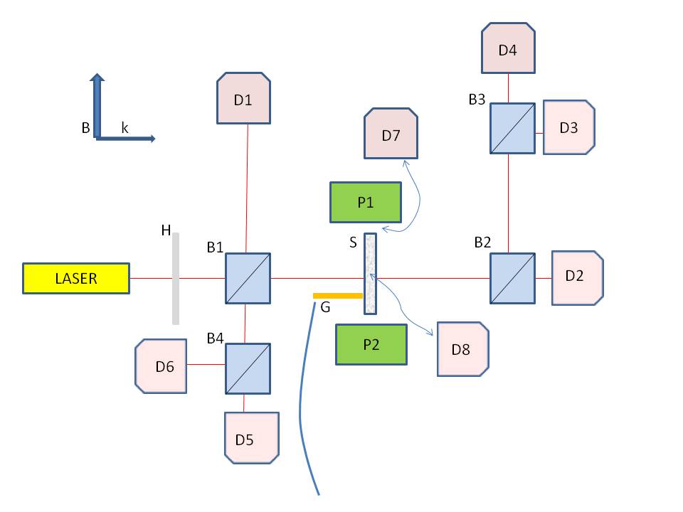
Figure 2: Schematic of the experimental setup, showing sample (S) kept between the pole pieces P1 and P2 of an electromagnet. G is the Gauss Probe, H the half-wave plate, D1-D8 detectors, and B1 and B2 are non-polarising beam splitters while B3 and B4 are polarising beam splitters. Arrows B and k denote the directions of the applied magnetic field and the wave-vector of the incident light.

We have measured the reflected and the transmitted intensities and their polarisations upon irradiation of our ferrofluid by a $633nm$ light from a $5mW$ cw He-Ne laser. The ferrofluid (Ferrolabs, USA) consisted of surfactant coated $Fe_{3}O_{4}$ nanospheres of radius $a_{NP}$ ($\sim 10nm$) randomly dispersed in kerosene. Figure 2 is the schematic of our apparatus. Linearly polarised light from the laser source (the plane of polarisation of which could be rotated by means of the halfwave plate, H) was incident on the sample (S) that was contained in a glass cuvette of size $1cm\times 1cm\times 2mm$ ($2mm$ along the direction of incident light). A non-polarising beam-splitter (B1) placed in the path of the incidence allowed us to monitor the intensity of the incident light using detector D1 and that of the reflected light using detectors D5 and D6. The cuvette was held between the pole pieces (P1 and P2) of an electromagnet that could produce a tunable magnetic field tranverse to the direction of incidence of light, of upto  450G, uniform over the illuminated sample to within a few mG, as measured by the Hall-effect Gauss probe (G). The light transmitted through the sample was incident on a non-polarising beam-spiltter (B2); detector D2 provided a measure of the transmitted intensity while the combination of the polarising beam-splitter (B3) and detectors D3 and D4 enabled the determination of its plane of polarisation. Similarly, using polarising beam splitter B4 and detectors D5 and D6, the intensity and polarisation of the reflected light could be determined. Detectors D1 - D6 were identical photodetectors (Thorlabs DET110). A small photodiode (D7) was placed in the narrow gap between the electromagnet and the cuvette in order to measure the light intensity scattered to the side. A similar detector (D8) placed on top (perpendicular to both the direction of light incident on the sample and to the applied magnetic field) was used to measure the light intensity scattered in that direction.

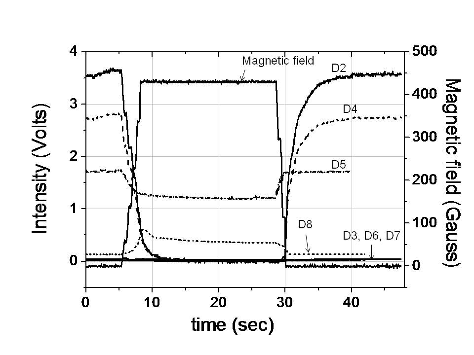
Figure 3: Oscilloscope traces showing, as function of time, the applied magnetic field and the light intensities as measured by detectors D2-D8. The inensity of the transmitted light reduces to zero when the magnetic field is increased; that of the reflected light is found to decrease to a smaller extent. Both the transmitted and the reflected light retain the incident linear polarisation, in this case horizontal polarisation.

Figure 3 shows the relative variation of the reflected and the transmitted intensities and their polarisations with applied magnetic field. In this case the incident light is horizontally polarised (i.e., plane of polarisation perpendicular to the incident wave-vector, k, and parallel to the applied magnetic field, B). A simultaneous decrease in both the transmitted light (D2) and the reflected light (D5) is observed as the applied field is increased. While the transmission drops to near-zero, the reduction in the reflection is less pronounced. On decreasing the magnetic field back to zero, the original intensities are recovered. The intensities recorded on detectors D4 and D5 (horizontal polarisation) and D3 and D6 (vertical polarisation) confirm that the transmitted and the reflected light retain the input (horizontal) polarisation. The scattered intensities in the transverse directions (D7, D8) are quite small. The situation was quite similar when the plane of polarisation of the incident light was perpendicular to the applied magnetic field (i.e., vertical).
The experiment was then repeated for two other wavelengths - (a) $612nm$ (He-Ne laser) for which the fall of the intensities with increasing magnetic field was slower than that for the $633nm$ wavelength, and (b) for $780nm$ (diode laser) for which too, the fall of intensity was slower than that for $633nm$ light. As we shall see below, these experimental observations are all qualitatively consistent with what is expected from our 1D model.

V Discussion

We now consider more explicitly how the applied magnetic field tunes the scattering properties of the ferrofluid. There is ample evidence that the nanoparticles (nanomagnets) rearrange to form spatially ordered structures, like linear chains directed along the magnetic field Abraham ; Butter ; Li1 ; Li2 . An overall spatial ordering of the nanoparticles is to be expected on general grounds as resulting from the minimization of the total energy of the magnetostatic coupling of the nanomagnetic particles with the externally applied magnetic field, and the magnetic dipolar interaction between these nanomagnets. The permanent magnetic dipole moment of these single domain magnetite nanoparticles is  $5\times 10^{4}$ Bohr magneton. The magnetostatic energy per nanoparticle in the external magnetic field of $300G$ is about $0.1eV$, exceeding both the thermal energy ($k_{B}T$), and the inter-dipolar interaction magnetic energy per nanoparticle. This implies that the external magnetic field can indeed introduce spatial ordering of these nanomagnets. Thus, by varying the external magnetic field, we can expect to continuously tune the spatial order (wave-vector $Q$), sweeping across the Bragg resonance condition ($Q$ = 2$k_{0}$, i.e., $q=2$), leading to strong scattering. The strong scattering (small mean free path) enhances the time taken by light to transit through our LAB cavity. This should result in a dip in the transmission and the reflection coefficients bracketing the Bragg condition, as indeed our simulations (Fig. 1) show and our experiments (Fig. 3) reaffirm. As noted before (following Eq. 1) the asymmetric decrease of the two intensities arises from the simple fact that light is incident from one end of the sample, and is not injected directly well within the sample (LAB).
Encouraged by this qualitative agreement between the numerical results of our 1D-model simulation and the experimental observations on our 3D ferrofluid, we now proceed to examine if the choice of the parameter values for the model (specifically, $\eta_{OR},\eta_{P},\eta_{I}$) do indeed correspond reasonably well to our experimental ferrofluid. The input parameters taken for the ferrofluid in the experiment are: nanoparticle mean number density $n_{FF}\simeq 10^{16}cm^{-3}$, nanoparticle radius $a_{NP}\simeq 15$ nm, dielectric constant of the nanoparticle material $Fe_{3}O_{4},\epsilon_{NP}=4+i2.2$, and the dielectric constant of the suspension medium (kerosene) $\epsilon_{K}=1.8$. The above parameters straightforwardly give the mean dielectric constant (the real part used in Eq. 4 and 5,

$$\epsilon_{0}=\epsilon_{K}(1-{{4\pi}\over{3}}n_{FF}a_{NP}^{3})+Re(\epsilon_{NP}){{4\pi}\over{3}}a_{NP}^{3}n_{FF}\simeq 2.1$$ (6)

Next, the dissipation parameter :

$$\eta_{I}=\epsilon_{I}/\epsilon_{0}=Im(\epsilon_{NP}){\frac{4\pi}{3}}n_{FF}a_{NP}^{3}\simeq 0.31.$$ (7)

The random disorder parameter $\eta_{OR}$, arises out of the fluctuations of the local number density of nanoparticles. Assuming a Poissonian distribution for the fluctuations and making use of the fact that the variance equals the mean (both taken over the length scale of a wavelength), we obtain

$$\eta_{OR}^{2}=32\pi^{2}(Re\epsilon_{F}-\epsilon_{k})^{2}({\frac{4\pi}{3}}a_{NP}^{3})^{2}({\frac{n_{FF}}{\lambda_{0}^{3}}})\simeq 0.037<<1,$$ (8)

as expected for a dense random system (${{4\pi}\over{3}}\lambda^{3}_{0}n_{FF}\gg 1$). This again is consistent with the fact that the dense random system is not, by itself, an effective scatterer – it is the spatial modulation (Bragg scattering) that makes the overall scattering effectively strong.

The simultaneous minima of transmission and reflection at $q=2$ in Fig.2 is a clear signature of the Bragg resonance condition, and is consistent with the ferrofluid parameters. This can be seen from the following geometrical considerations based on the fact that in a magnetic field ($\sim$ 100 G) the nanoparticles are known to re-arrange forming chains aligned parallel to the field Abraham ; Butter ; Li1 ; Li2 . Assuming that the overall number density of the ferrofluid remains unchanged, we have $1/n_{FF}=2a_{NP}d^{2}$, where $2a_{NP}$ is the nanoparticle spacing along the chains and $d$ the interchain separation. This gives $d\sim$half the wavelength of light, $\lambda_{0}$ in the medium, and thus closely corresponds to the Bragg condition. From the same geometrical considerations, the parameter $\eta_{P}$, giving the depth of the periodic dielectric modulation under the above Bragg condition, can be readily estimated. It is given by $\eta_{P}=(16\pi/3)(\epsilon_{NP}/\epsilon_{K})(n_{FF}a_{NP}^{3})\simeq 1$. Overall, given the complexity of the system and the simplicity of our model, we find the above estimates of the various parameters quite consistent with our experiments.

Next we turn to polarisation, namely, how, despite multiple scattering, the transmitted as well as the reflected light retains the incident linear polarisation. Let us consider the case of transmission, where the initial and the final wave-vectors are parallel. For clarity, we resolve the linearly polarised light into its left and the right circularly polarised components, both of which traverse the same path-length in the optical medium, and, therefore, undergo the same dynamical phase shift. This causes no change in the state of polarisation. Phase shifts, however, do also arise as a result of the geometric phases suffered by the two circularly polarised components. These phase shifts are equal and opposite for the left and the right components, and have a magnitude given by the solid angle subtended at the origin in the space of directions traced out by the ray trajectory. For light, with photon spin =1, this does lead to a rotation of the plane of linear polarisation by half that solid angle, which is, of course, random for our disordered system. In the present case, however, the scattering is dominated by the Bragg scattering which is essentially in the forward and the backward directions. These multiple scatterings subtend zero solid angle, and hence give no rotation (due to the geometric phase) of the plane of incident linear polarisation for the transmitted (forward) and the reflected (backward) scattered light. Moreover, recall that a single scattering by a Rayleigh scatterer (our spherical nanoparticle) retains the incident linear polarisation of light, anyway. Besides, unlike the case in Li1 ; Li2 , our magnetic field is transverse to the direction of incidence, and hence there is no Faraday rotation. As already noted, in the transverse directions, the light intensities are very small.
Finally, our model can be viewed in a broader perspective: some of the quantities of possible physical interest become calculable. It is possible to calculate the photon transit time ($\tau_{L}$) in our LAB cavity. Indeed, the introduction of a weak dissipation ($\ell_{i}$) provides an effective measure Anantha for $\tau_{L}$, which can be readily shown to be given by $e^{-\tau_{L}c_{0}/\ell_{i}}=(\left|T\right|^{2}+\left|R\right|^{2}$). Also, the amount of light energy stored ($U_{S}$) in our LAB cavity under steady-state illumination (intensity $I$) can then be readily expressed as $U_{S}=I\tau_{L}$. We note that this light is stored as light, and not as an electronic excitation. It is tempting to suggest here that this stored light may re-emerge from the LAB cavity as a flash if the magnetic field (and, therefore, the confining strong scattering) could be switched off instantaneously. This, of course, assumes that the nanoparticles in the ferrofluid relax back sufficiently fast. The emergent light pulse would have a linear polarisation same as that of the incident light. Clearly, this would not be the case if the light had been stored as an electronic excitation, and re-emitted as fluorescence.

VI Summary

In summary, we have studied experimentally as well as theoretically light transmission through and its reflection from a magneto-statically tunable ferrofluid. We have developed a mechanism in terms of scattering of light in a disordered medium in the presence of weak dissipation, where the scattering could be effectively enhanced by a spatial periodic modulation of the background dielectric constant, giving Bragg scattering. Our theoretical treatment of transmission and reflection of light is based on the method of invariant imbedding. The key idea to emerge from our studies is that the strong multiple scattering of light and the resulting small mean free path can give rise to a long photon sojourn time, thereby effectively making our ferrofluid system akin to a lossy cavity. It is apt to point out here that the increased photon sojourn time calculated and reported in this work comes from multiple scattering because of disorder, re-inforced by Bragg scattering due to spatial modulation. It does not arise because of dispersion as in the well-known slow-wave systems, where the slowness comes essentially from the fast variation of the real part of the refractive index with frequency, as, for example, in the Electromagnetically Induced Transparency (EIT) systems, where very low group velocities (as low as few $cms^{-1}$ could be achieved over a narrow frequency window Hau . Given the recent research activity Mehta ; Kalpakkam ; Li1 ; Li2 in the magneto-optical properties of magnetically tunable ferrofluids, the present work seems to be of some interest.

VII Acknowledgement

One of us (M. S.) wishes to acknowledge the Raman Research Institute for extensive use of the experimental facilities and for hospitality during the course of this work.

References

- (1) Anderson P. W. Phys. Rev. 109 1492 (1958).
- (2) Sheng P., Introduction to Wave Scattering, Localization and Mesoscopic Phenomena Academic Press, New York (1995).
- (3) see for example, Graham M., Adkins C. J., Behar H. and Rosenblaum R. J. Phys. : Cond. Matter 10 809 (1998).
- (4) John, S., Phys. Today, 44, 32 (1991).
- (5) John, S., Phys. Rev. Lett.58 2486 (1987).
- (6) Kumar N., Phys. Rev. B31 5513 (1985).
- (7) Ramal R. and Doucot B., J. d’Physique 48 509, (1987).
- (8) Abraham V. S., Swapna Nair, Rajesh S., Sajeev U.S. and Anantharaman M. R. Bull. Mater. Sci. 27 155 (2004).
- (9) Butter K., Bomans P. H., Frederik P. M., Vroege G. J. and Philipse A. P. Nature Matl. 2, 88 (2003).
- (10) Li J., Liu X., Lin Y., Qui X., Ma X. and Huang Y. J. Phys.D: Appl. Phys. 37, 3357 (2004).
- (11) Li J., Liu X., Lin Y., Bai L., Li Q. and Chen X. Appl. Phys. Lett. 91, 253108 (2007).
- (12) Anantha Ramakrishna S. and Kumar N., Phys. Rev. B61, 3163 (2000).
- (13) Hau L.V., Harris S.E., Zachary Dutton and Cyrus Behroozi Nature 397 594 (1999).
- (14) Mehta R. V., Rajesh Patel, Rucha Desai, Upadhyay R. V. and Kinnari Parekh, Phys. Rev. Lett. 96, 127402 (2006), see, however, Hema Ramachandran and Kumar N. Phys. Rev. Lett. 100 229703 (2008).
- (15) Laskar J. M., Philip J. and Baldev Raj Phys. Rev. E78, 031404 (2008).