Demonstration of quantum Zeno effect in a superconducting phase qubit

Abstract

Quantum Zeno effect is a significant tool in quantum manipulating and computing. We propose its observation in superconducting phase qubit with two experimentally feasible measurement schemes. The conventional measurement method is used to achieve the proposed pulse and continuous readout of the qubit state, which are analyzed by projection assumption and Monte Carlo wave-function simulation, respectively. Our scheme gives a direct implementation of quantum Zeno effect in a superconducting phase qubit.

Quantum Zeno effect (QZE), proposed by Misra and Sudarshan in 1977 Misra , is a paradigm showing that quantum physics is counter-intuitive. It predict that if the state of a unstable or oscillating quantum system is measured frequently to see whether it still stay at a initial state, transitions from the initial state to other states will be suppressed or even inhibited. Since then, many exciting progresses have been made both theoretically and experimentally. In the theoretical side, physicist interpret it with wave-function collapse assumption in early days Cook ; Itano , which is shown to be not necessary Frerichs . Later, it was generalized in a few different ways. Concerning the measurement, it can not only retard incoherent decay but also coherent Rabi oscillation. On the other hand, for unstable system, frequent measurements may even also enhance the decay rate under some conditions, which is the so-called quantum anti-Zeno effect Fischer ; Kofman ; Facchi . As to the readout aspect, one can adopt pulse or continuous measurements L. S. Schulman ; Streed . In the experimental side, QZE have been demonstrated in many systems, such as trapped ions Itano , optical lattice Fischer , Bose-Einstein condensate Streed , microwave cavity Bernu , etc.

Studying QZE is very important. Beyond the interest of fundamental physics, it has many practical applications. These includes reducing decoherence in quantum computing Facchi05 ; Franson ; Hosten , efficient preservation of spin polarized gases Nagels , keeping system stay in object subspace Barenco . There are interesting explorations of applications in superconducting qubit systems, e.g., generation of entangled state X.-B. Wang and implementation of quantum switch Zhou . Recently, the possibility of observing QZE in superconducting qubits is proposed Lizuain ; Matsuzaki . However, demonstration of QZE in superconducting system is very difficult because of the lacking of competent measurement method. Conventionally, it was observed with quantum non-demolition (QND) readout. In circuit Quantum Electrodynamics (CQED), state of the qubit could be imprinted on the cavity field state in a QND readout, but the signal-to-noise ratio is so low that we must repeat considerable times to complete the QND readout. Thus, a recent experiment A. Palacios-Laloy demonstrate QZE qualitatively in CQED can not guarantee its practical applications due to the noise. Here, we suggest experimental feasible schemes to demonstrate QZE in a superconducting phase qubit with both pulse and continuous measurement strategy instead of QND readout.

Since the quadratic decay behavior (prerequisite for QZE) in the initial decay stage of the qubit excited state has not been observed yet, suppressing of energy relaxation in superconducting qubit is not accessible technically. Thus, we here focus on another case of QZE, i.e., suppressing the unitary evolution of the phase qubit. There are at least two feathers that differentiate our schemes from those implemented in other systems. Firstly, the measurement method used here is the so called selective measurement instead of QND readout which is still a big challenge to realize continuous measurement in superconducting qubits system. Secondly, our schemes are immune from the relaxation of the qubit by using an appropriate initial state. That is rather necessary in the context of the very short energy relaxation time of superconducting qubits. It should be noticed that, besides the function of demonstrating the basic phenomenon of quantum mechanics, our proposal can lay a foundation for the applications of QZE in quantum information processing, e.g., Ref. X.-B. Wang .

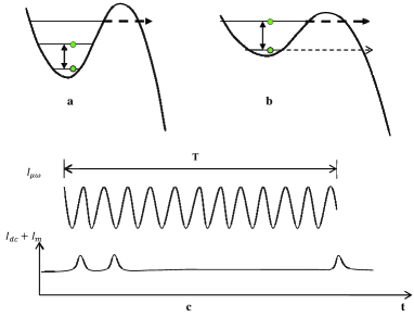
Figure 1: Energy levels in the potential well when measurement pulses is off (a) and on (b); c, indication of the bias of the phase qubit, including microwave driving $I_{\mu w}$ (upper) and dc bias current with measurement pulses (down).

Superconducting phase qubit usually consists of a large current-biased Josephson junction (JJ). When the bias current approaches its critical current, there exist several no-degenerate energy levels in each well of the washboard potential of the qubit, see Fig. 1(a). The lowest two states act as a qubit, which is the so-called phase qubit. Experimentally, it can be easily controlled by bias cunrrent containing both dc and microwave components Martinis .

An advantage of phase qubit over other types of superconducting qubit is its built-in readout. It relies on the possibility that the qubit states in the potential can tunnel through the potential barrier into continuum outside. The tunneling rate of one level usually differ dramatically from the other one at least two orders of magnitude Martinis09 . So the ground and excited state can be mapped to no-tunneling and tunneling case, respectively. Experimentally, one can lower the barrier so that the excited state of the qubit can tunnel through the barrier quickly but the ground state can’t, see Fig. 1(b). Therefore, one can add a pulse to the bias Cooper , see Fig. 1(c), so that the height of the barrier only fitting the excited qubit state.

Now, we begin our pulse measurements scheme. When operating the phase qubit for quantum gates, the bias is tuned to an appropriate value so that there are three or four levels in the potential well as shown in Fig. 1(a). In this case, neither of the qubit states could tunnel outside. Drive the phase qubit with a resonant microwave, the qubit will oscillate between the ground and excited state with a period of $2\pi/\Omega$. If the initial state is the ground state, after half a period, the qubit is driven to the excited state. To demonstrate QZE, we superpose a series of short uniform measurement pulses to the qubit bias, see Fig1. (c). Because the pulse during time $\tau$ is much smaller than the oscillating period, we consider that the probe pulse is instantaneous. To be more specifically, in half a period of Rabi oscillation $T=\pi/\Omega$, there are $n$ evenly distributed pulses with the time interval as $\delta t=T/n$.

According to the Hamiltonian, we can calculate straightforwardly the population of the ground state $|0\rangle$ at $t=\delta t$, before the first pulse, as $P_{0}^{-}(\delta t)=\cos^{2}\left(\pi/2n\right).$ After the first probe, the probability of no-tunneling $P_{0}^{1}$, i.e, the probability of the qubit collapsing to ground state, equals to $P_{0}^{-}(\delta t)$. So, after all the $n$th probes, the survival probability of the initial ground state $|0\rangle$ is $P_{0}^{n}=\left(P_{0}^{1}\right)^{n}=\left[\cos^{2}\left(\pi/2n\right)\right]^{n}.$ When $n\gg 1$, making the proximation of $\cos\left(\frac{\pi}{2n}\right)\approx 1-\left(\pi/2n\right)^{2}$ and using the relation $\underset{n\rightarrow\infty}{\lim}(1-x/n)^{n}=e^{-x},$ one gets

$$P_{0}^{n}=\exp\left({-{{\pi}^{2}\over 4n}}\right).$$ (1)

We have plotted the survival probability with both expressions in Fig. 2, which shows that the approximation to exponential function is perfect when $n>10$. Obviously, with the increasing of $n$, the survival possibility of initial state tends to 1, which is one kind of QZE.

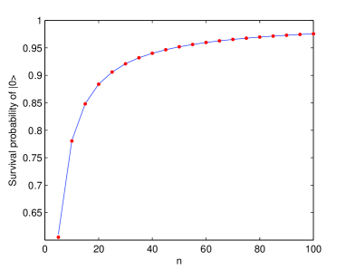
Figure 2: Survival probability of $|0\rangle$ in a half period of Rabi oscillation vs. number of probes. Red dots is plotted with $P_{0}^{n}=\left[\cos^{2}(\pi/2n)\right]^{n}$, and solid line with $P_{0}^{n}=\exp({-{\pi}^{2}/4n})$. The approximation to exponential function is perfect when $n>10$.

Although it is similar with the experiment with trapped ions Itano , there has significant difference between them. In their experiment, they use a series of QND measurements during the Rabi oscillation and measure the final state of the trapped ions at the end of a half oscillating period. Therefore, even if some measurement results are not the initial state, the qubit still evolve according to Hamiltonian after the measurements. Thus, there exist a small probability to return to the initial state at last. Instead, we employ a selective measurement approach to obtain the probability that all the probes get the same result, i.e, the initial ground state. This is achieved by the fact that if the result is other than the initial state, the JJ will switch to a non-zero voltage state, which means that the state of qubit will be destructed and stop evolve after the probe. It should be noted that our scheme exhibit what Misra and Sudarshan first called QZE Misra .

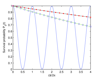
Figure 3: Survival probability of $|0\rangle$ vs. time. Blue solid line is showing Rabi oscillation without any decay. Green and black line is plotted according to $\cos^{2n}(\Omega\delta t/2)$ with $\delta t=\pi/50\Omega$, $\pi/100\Omega$, respectively. Purple circle and red dot denote $\exp((-\Omega^{2}\delta t/4)t)$ with corresponding $\delta t$ as above.

It is well known that when the interval time among the measurement pulses is very small, the survival probability of the initial state reduces exponentially with the increasing of time. Similarly, we can easily get

$$P_{0}(t)=p_{0}^{n}\approx\exp\left[\left(-{\Omega^{2}\delta t\over 4}\right)t\right]$$ (2)

with $t=n\delta t$. We have plotted $P_{0}(t)$ with $\delta t=\pi/50\Omega$, $\pi/100\Omega$ in Fig. 3. Instead of normal Rabi-type oscillation, the initial state $|0\rangle$ decay exponentially with an effective characteristic time $t_{c}$

$${1\over t_{c}}={\Omega^{2}\delta t\over 4}.$$ (3)

It is a very important characteristic parameter showing that to what extent the probes suppress the state transition. When $\delta t=\pi/50\Omega$, $t_{c}=200/\pi\Omega$, which is much larger than the characteristic time of Rabi oscillation $1/\Omega$, we can also see from Eq. (3) that the decay time is inverse function of $\delta t$.

Then, we move to the feasibility of the above pulse measurements scheme. Theoretically, the more frequently a qubit state is observed, the more likely it will be inhibit to transition to other state from the initial state. However, in practice, there are three main obstacles stopping us from beating the QZE limit. Firstly, measurement fidelity is always lower than unit; secondly, each measurement is not instantaneous but inevitably lasts for a finite period of time; and finally, the finite decoherence time of the qubit.

The measurement of phase qubit state is achieved by using its macroscopic quantum tunnel. The imperfect fidelity is induced from the finite ratio of the tunneling rates of $|1\rangle$ and $|0\rangle$ states. It’s believed that the ratio is typically around $200$ Martinis09 . During the measurement pulse, the tunneling possibility from the excited state is close but a little bit lower than 1, while that of the ground state is a small but nonzero quantity. However, this measurement have single shot readout fidelity up to 96% theoretically Martinis09 , which is the highest among all the known readout approaches of superconducting qubits.

The other bothering factor is that the readout can’t be accomplished instantaneously. In a measurement process, the added probe pulse alters the level structure of the qubit, making it detuning from the driving microwave. The question how to judge the suppression of the oscillation comes from QZE or from the reduce of the effective driving time is unavoidable to any experimental scheme of demonstrating QZE. Actually, for larger measuremnt times $n$, the sum of the measurement periods is not negligible compared to the duration of the whole process. Therefore, part of the decrease in the transition probability is due to the decrease in the time during which the qubit is resonant driven. For an extreme case of $n=100$, the sum of the measurement periods is 50% of the total time $T$. Even for this case, the survival probability of the initial state is as high as 97%, which is much higher than that of sole resonant driven. So we can safely conclude that the suppression of the oscillation mainly comes from QZE.

Finally, the decoherence including relaxation and pure dephasing of the qubit is usually considered as bottle-neck for illustrating QZE. From now on, we would clarify why it can be neglected in our scheme. On the one hand, pure dephasing can be ignored after noticing that the interval between two nearest measurements is very short compared with the dephasing time which could be as long as hundreds of $ns$. On the other hand, the lifetime of an average phase qubit is $T_{1}=600$ n$s$. If $T$ can be much smaller than $T_{1}$, to avoid the decay of the excited state, then the experiment will be able to carried out easily. But that is not necessary for observing QZE. The reason is that before each probe, the average population of excited state is much lower than 1, i.e.,

$$P_{1}=\frac{1}{\tau}\int_{0}^{\tau}\sin^{2}(\Omega t/2)dt=\Omega^{2}\tau^{2}/12\ll 1.$$ (4)

To be more specifically, $P_{1}\simeq 0.07$ for $n=32$, i.e., each probe will project the qubit sate to the ground sate subspace with high probability. Therefore, the qubit state can only has a small probability to excite to the excited sate, which means we will have a much longer effective lifetime for the excited state in our scheme. If we conservatively choose $T=T_{1}=600$ n$s$ and each probe pulse lasts $t_{p}=3$ n$s$, then the ratio between the measurement time and the total oscillating time is $T/t_{p}=200$. In the trapped ions experiment, the quantity is about 100. With a larger ratio, one can implement more probes within a half period of Rabi oscillation. So, we strongly believe that QZE can be verified definitely in phase qubit with our pulse measurement method.

Next, we propose to demonstrate QZE in a phase qubit by continuous measurement. Theoretically, Heisenberg uncertainty principal limits how frequently a measurement can be performed. However, one could also adopt continuous measurement approach to observe QZE. The main difference of the continuous measurement approach from the above pulse measurement scheme is that the bias is fixed to only allow the excited state to tunnel outside during the oscillation of the qubit. This is reasonable since the tunneling rate of the excite state is two orders of magnitude larger than that of the ground stateMartinis09 . Furthermore, the tunneling rate of the ground state is also smaller than the Rabi frequency of the qubit in our parameter figuration. Therefore, we do not need to take the rare tunneling event of the ground state into account. The system is initially prepared in the ground state; a resonate microwave is driving the phase qubit between the ground and excited state. The life time of the excited state due to spontaneous decay is much longer because of quantum tunneling is very fast. Neglecting the spontaneous decay term, we get a Hamiltonian describing this dissipative system in interaction picture is

$${{H}_{I}}=\left(\begin{matrix}0&\Omega\\ \ \Omega&-i\Gamma/2\end{matrix}\right).$$ (5)

Before going into QZE, we would like to discuss how continue measurement works. In our case, the excited state has a tunneling rate $\Gamma$, but the ground state can’t tunnel, which means in a short time interval $\delta t$, the excited state tunnel with the possibility of $\Gamma\delta t$. If a tunneling count, we know the qubit state before tunneling is the excited state; otherwise we can’t discern the ground and excite state, but what we can get from the interrogation is that the qubit is more likely in ground state at the end of $\delta t$ than at the beginning. This point is the the essential of Monte Carlo wave-function method, which is developed for simulating open system Blatt ; Molmer ; Yu-Wen . Below we use this method to show QZE and compare it to the analytical result.

Back to the Hamiltonian in Eq. (5). If $\Gamma=0$, the qubit is absolutely populates $|1\rangle$ at $t=T=\pi/2\Omega$. Now, we suppose $\Omega\ll\Gamma$. The non-Hermitian Hamiltonian can be simulated with Monte Carlo wave-function method. The procedure can be summarized as follows: (1). Discretize the time interval $T$ by a very small time step $\delta t$. (2). Determine the probability of tunneling $P=\Gamma\delta t|\langle 1|\psi\rangle|^{2}$, choosing $\delta t$ to make sure $P\ll 1$. (3). Obtain a random number $r$ distributed uniformly between zero and one, and compare it with $P$. (4). If $r<P$, there is a tunneling, the system switch to finite voltage state, and this run is end. Then start next run from step 1. If $r>p$, no tunneling takes place, the qubit evolves under the influence of the non-Hermitian Hamiltonian described by Eq.(5) and the qubit state at the end of $\delta t$ is

$$|\psi(t+\delta t)\rangle=(1-\frac{iH\delta t}{\hbar})|\psi(t)\rangle/||(1-\frac{iH\delta t}{\hbar})|\psi(t)\rangle||$$ (6)

where we have approximately expand the the evolution operator to first order of $\delta t$. (5). Repeating the process, we can get a trajectory of the qubit state.

It is obvious that if no tunneling appears in the whole period $T$, the qubit state will totally stay in the state of $|0\rangle$ at the end of the probed oscillation. So, the survival probability of a initial state is same as that of no tunneling during the period. We simulate many times for a certain $\Gamma$ to obtain survival probability $P_{0}$. Furthermore, we have studied the relation between $P_{0}$ and $\Gamma$ as shown in Fig. 4.

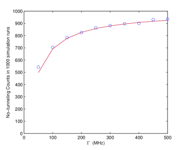
Figure 4: No-tunneling counts vs tunneling rate of the excited state. Monte Carlo wave-function simulation parameters are $\Omega=2\pi\times 1$ MHz, $T=\pi/2\Omega$ and $\Gamma\in[50,500]$ MHz. The blue circles are data from simulation, and the red solid line is plotted according to the analytical expression in Eq. (8).

The Hamiltonian in Eq. (5) can also be solved analytically. The evolution operator of the dissipative two-level system has the form of

$$U=e^{-iH_{I}t}e^{-\frac{\Gamma}{4}t}\left[\cosh(ht)-i\frac{\bm{h}\cdot\bm{\sigma}}{h}\sinh(ht)\right]$$ (7)

where $h=\sqrt{(\Gamma/4)^{2}-\Omega^{2}}$ and we have assumed that $\Gamma/4>\Omega$. If the initial state is $|0\rangle$, then the survival amplitude is function of time and has the form of

$$A_{0}(t) = \langle 0|e^{-iH_{I}t}|0\rangle$$ (8)

$$= e^{-\frac{\Gamma}{4}t}\left[\cosh(ht)+\frac{\Gamma}{2h}\sinh(ht)\right].$$

We have also plotted the survival probability of the initial state with this analytical expression in Fig. 4. We can see the Monte Carlo wave-function simulation is agree with the analytical result perfectly. More importantly, they both imply QZE as explained in the following. With the increasing of the excited state tunneling rate, the no-tunneling counts approaching to 1000, which is the total simulation runs’ number. We conclude that the survival probability of the initial state $|0\rangle$ is more strengthened with larger tunneling rate of the excited state. That is the essential meaning of QZE of a system measured continuously.

Additionally, we can also investigate the relation of pulse and continuous scheme in the future experiment. Theoretically, it could be proved that if the effective decay times of the initial state in the two schemes are the same, the interval between two sequential measurements in pulse scheme and decay rate of the excited state in continuous scheme should satisfy the relation L. S. Schulman of $\delta t\cdot\Gamma=4$. That is an important relationship between the two schemes.

We have proposed two schemes to observe QZE in a superconducting phase qubit: pulse and continuous measurement schemes. They are easy and feasible for up-to-date technique. Our result show that QZE can be demonstrated with the schemes more clearly than the trapped ions experiment. Since QZE is essential in the implementation of quantum information, the generalization of the proposed scheme to other kinds of superconducting qubits Makhlin ; Zhu is desirable.

We thank Prof. S.-L. Zhu for many helpful suggestion. This work was supported by the NSFC (No. 11004065), the SKPBR of China (No. 2011CB922104), the NSF of Guangdong Province (No. 10451063101006312), and the Startup Foundation of SCNU (No. S53005).

References

- (1) B. Misra and E. C. G. Sudarshan, J. Math. Phys. Sci. 18, 756 (1977).
- (2) R. J. Cook, Phys. Scr. T21, 49 (1988).
- (3) W. M. Itano, D. J. Heinzen, J. J. Bollinger, and D. J. Wineland, Phys. Rev. A 41, 2295 (1990).
- (4) V. Frerichs and A. Schenzle, Phys. Rev. A 44, 1962 (1991).
- (5) M. C. Fischer, B. Gutiérrez-Medina, and M. G. Raizen, Phys. Rev. Lett. 87, 040402 (2001).
- (6) A. G. Kofman and G. Kurizki, Nature (London) 405, 546 (2000).
- (7) P. Facchi, H. Nakazato, and S. Pascazio, Phys. Rev. Lett. 86, 2699(2001).
- (8) L. S. Schulman, Phys. Rev. A 57, 1509(1998).
- (9) E. W. Streed, J. Mun, M. Boyd, G. K. Campbell, P. Medley, W. Ketterle, and D. E. Pritchard, Phys. Rev. Lett. 97, 260402 (2006).
- (10) J. Bernu, S. Deléglise, C. Sayrin, S. Kuhr, I. Dotsenko, M. Brune, J. M. Raimond, and S. Haroche, Phys. Rev. Lett. 101, 180402 (2008).
- (11) O. Hosten, M. T. Rakher, J. T. Barreiro, N. A. Peters, and P. G. Kwiat, Nature (London) 439, 949 (2006).
- (12) J. D. Franson, B. C. Jacobs, and T. B. Pittman, Phys. Rev. A 70, 062302 (2004).
- (13) P. Facchi, S. Tasaki, S. Pascazio, H. Nakazato, A. Tokuse, and D. A. Lidar, Phys. Rev. A 71, 022302 (2005).
- (14) B. Nagels, L. J. F. Hermans, and P. L. Chapovsky, Phys. Rev. Lett. 79, 3097 (1997).
- (15) A. Barenco, A. E. Berthiaume, D. Deutsch, A. Ekert, R. Jozsa and C. Macchiavello, SIAM J. Comput 26, 1541 (1997).
- (16) X.-B. Wang, J. Q. You, and F. Nori, Phys. Rev. A 77, 062339(2008).
- (17) L. Zhou, S. Yang, Y.-X. Liu, C. P. Sun, and F. Nori, Phys. Rev. A 80, 062109 (2009).
- (18) J. Gambetta, A. Blais, M. Boissonneault, A. A. Houck, D. I. Schuster, and S. M. Girvin, Phys. Rev. A 77, 012112(2008).
- (19) I. Lizuain, J. Casanova, J. J. Garcia-Ripoll, J. G. Muga, and E. Solano, Phys. Rev. A 81, 062131 (2010).
- (20) Y. Matsuzaki and K. Semba, Phys. Rev. B 82, 180518(R) (2010)
- (21) A. Palacios-Laloy, F. Mallet, F. Nguyen, P. Bertet, D. Vion, D. Esteve, and A. N. Korotkov, Nature Physics 6, 442 (2010).
- (22) J. M. Martinis, S. Nam, J. Aumentado, and K. M. Lang, Phys. Rev. B 67, 094510 (2003).
- (23) J. M. Martinis, Quant. Inf. Process 8, 81 (2009).
- (24) K. B. Cooper, M. Steffen, R. McDermott, R. W. Simmonds, S. Oh, D. A. Hite1, D. P. Pappas, and J. M. Martinis, Phys. Rev. Lett. 93, 180401 (2004).
- (25) M. B. Plenio and P. L. Knight, Rev. Mod. Phys. 70, 101(1998); R. Blatt and P. Zoller, Eur. J. Phys. 9, 250 (1988).
- (26) K. Mølmer, Y. Castin, and J. Dalibard, J. Opt. Soc. Am. B 10, 524 (1993).
- (27) Y. Yu, S. L. Zhu, G. Sun, X. Wen, N. Dong, J. Chen, P. Wu, and S. Han, Phys. Rev. Lett. 101, 157001 (2008); X. Wen, S. L. Zhu, and Y. Yu, Phys. Rev. B 80, 094507 (2009).
- (28) Y. Makhlin, G. Schon, and A. Shnirman, Rev. Mod. Phys. 73, 357 (2001).
- (29) S. L. Zhu, Z. D. Wang, and P. Zanardi, Phys. Rev. Lett. 94, 100502 (2005); S. L. Zhu, Z. D. Wang, ibid. 91, 187902 (2003).