Emergent Criticality Through Adaptive Information Processing in Boolean Networks

Abstract

We study information processing in populations of Boolean networks with evolving connectivity and systematically explore the interplay between the learning capability, robustness, the network topology, and the task complexity. We solve a long-standing open question and find computationally that, for large system sizes $N$, adaptive information processing drives the networks to a critical connectivity $K_{c}=2$. For finite size networks, the connectivity approaches the critical value with a power-law of the system size $N$. We show that network learning and generalization are optimized near criticality, given task complexity and the amount of information provided surpass threshold values. Both random and evolved networks exhibit maximal topological diversity near $K_{c}$. We hypothesize that this diversity supports efficient exploration and robustness of solutions. Also reflected in our observation is that the variance of the fitness values is maximal in critical network populations. Finally, we discuss implications of our results for determining the optimal topology of adaptive dynamical networks that solve computational tasks.

In 1948, Alan Turing proposed several unorganized machines made up from randomly interconnected two-input NAND logic gates turing69 as a biologically plausible model for computing. He also proposed to train such networks by means of a “genetical or evolutionary search.” Much later, random Boolean networks (RBN) were introduced as simplified models of gene regulation Kauffman69 ; Kauffman93 , focusing on a system-wide perspective rather than on the often unknown details of regulatory interactions Bornholdt2001 . In the thermodynamic limit, these disordered dynamical systems exhibit a dynamical order-disorder transition at a sparse critical connectivity $K_{c}$ DerridaP86 . For a finite system size $N$, the dynamics of RBNs converge to periodic attractors after a finite number of updates. At $K_{c}$, the phase space structure in terms of attractor periods AlbertBaraBoolper00 , the number of different attractors SamuelsonTroein03 and the distribution of basins of attraction Bastola98 is complex, showing many properties reminiscent of biological networks Kauffman93 . In cellular automata (CA), complex computation has been hypothesized to occur where the rules show complex dynamics at “the edge of chaos” langton1990 ; packard1988 . This claim was refuted in mitchell93 . However, the argument in mitchell93 rests on symmetric spaces in the CA lattice and rule space. These results therefore do not apply to RBN. Phase transition in information dynamics was studied in lizier2008 . State-topology coevolution in RBNs was studied by Kauffman:1991p959 ; BornholRohlf00 ; liu2006 and it was shown that networks evolved toward a critical connectivity $K_{c}=2$. This letter presents the first study to link complex dynamics, topology, and task solving in an open RBN.

In carnevali87a ; carnevali87b ; patarnello89 ; broeck90 simulated annealing (SA) and genetic algorithms (GAs) were used to train feedforward RBNs and to study the thermodynamics of learning. For a given task with predefined input-output mappings, only a fraction of the input space is required to train networks that generalize perfectly on all input patterns. This fraction depends on the network size and the task complexity. Moreover, the more inputs a task has, the smaller the training set needs to be to obtain full generalization. In this context, learning refers to correctly solving the task for the training samples while generalization refers to correctly solving the task for novel inputs. We use adaptation to refer to the phase where networks have to adapt to ongoing mutations (i.e., noise and fluctuations), but have already learned the input-output mapping. In this Letter, we study adaptive information processing in populations of Boolean networks with an evolving topology. Rewiring of connections and mutations of the functions occur at random, without bias toward particular topologies (e.g., feedforward). We systematically explore the interplay between the learning capability, the network topology, the system size $N$, the training sample $T$, and the complexity of the computational task.

First, let us define the dynamics of RBNs. A RBN is a discrete dynamical system composed of $N$ automata. Each automaton is a Boolean variable with two possible states: $\{0,1\}$, and the dynamics is such that ${\bf F}:\{0,1\}^{N}\mapsto\{0,1\}^{N},$ where ${\bf F}=(f_{1},...,f_{i},...,f_{N})$, and each $f_{i}$ is represented by a look-up table of $K_{i}$ inputs randomly chosen from the set of $N$ automata. Initially, $K_{i}$ neighbors and a look-table are assigned to each automaton at random. For practical reasons we restrict the maximum $K_{i}$ to $8$. An automaton state $\sigma_{i}^{t}\in\{0,1\}$ is updated using its corresponding Boolean function, $\sigma_{i}^{t+1}=f_{i}(\sigma_{i_{1}}^{t},\sigma_{i_{2}}^{t},...,\sigma_{i_{K_{i}}}^{t})$.

The automata are updated synchronously using their corresponding Boolean functions. For the purpose of solving computational tasks, we define $I$ inputs and $O$ outputs. The inputs of the computational task are randomly connected to an arbitrary number of automata. The connections from the inputs to the automata are subject to rewiring and are counted to determine the average network connectivity $\langle K\rangle$. The outputs are read from a randomly chosen but fixed set of $O$ automata. All automata states are initialized to “$0$” for each input pattern before simulating the network.

Methodology.— We evolve the networks by means of a traditional genetic algorithm (GA) to solve three computational tasks of varying difficulty, each of which defined on a $3$-bit input: full-adder (FA), even-odd (EO), and the cellular automata rule $85$ (R85) wolfram83 . The FA task receives two binary inputs $A$, $B$, an input carry bit $C_{in}$, and outputs the binary sum of the three inputs $S=A+B+C_{in}$ on the $2$-bit output and the carry bit $C_{out}$. The EO task outputs a $1$ if there is an odd number of $1$s in the input (independent of the order), a $0$ otherwise. R85 is defined for three binary inputs $A$, $B$, and $C$, and outputs the negation of $C$. The output for R85 task therefore only depends on one input bit. The EO task represents the most difficult task, followed by the FA and R85 task. Task difficulty is the complexity of information integration needed in the input to determine the output. This can be measured through information-theoretical decomposability of a task. We can represent the task itself as the contingency table of its inputs and outputs. Different decomposition models of the task are the different ways that we can calculate the marginal probabilities from the original contingency table zwick2004 . We calculate a weighted sum of the vector of the information content of all possible decomposition models of a task $F$. This can be summarized in: ${{decomposition}_{\text{F}}=\sum_{\text{m}\in Models_{F}}{\text{w}_{m}Inf_{m}}}$, where $Models_{F}$ is the set of all decomposition models of $F$, and the weight $w_{m}$ of a model is proportional to its degrees of freedom. The information content of a model is calculated using $Inf_{m}=1-\frac{\text{H}_{m}-\text{H}_{F}}{\text{H}_{ind}-\text{H}_{F}}$. Here, $H_{m}$ is the entropy of the model, $H_{F}$ is the entropy of $F$, and $H_{ind}$ is the entropy of the independence model (all input and output variables are assumed independent). Higher values for ${decomposition}_{F}$ mean that the task is more decomposable and therefore less difficult.

The genetic algorithm we use is mutation-based only, i.e., no cross-over operation is applied. For all experiments we ran a population of $30$ networks with initial connectivity $\langle K_{in}\rangle=1$ and a mutation rate of $0.8$. Each mutation is decomposed into $1+\alpha$ steps repeated with probability $p(\alpha)=0.5^{\alpha+1}$, where $\alpha\geq 0$. Each step involves flipping a random location of the look-up table of a random automata combined with adding or deleting one link. Each population is run for $30,000$ generations. We repeat each evolutionary run $30$ times and average the results. In each generation and for each tested input configuration, the RBN is run for a convergence time $t\propto N$ updates. Afterward, we run the network for an additional $t\propto N$ updates to record the activity of the output nodes. If the activity of an output node is “1” for at least half of the $t$ time steps, we interpret the output as a “1”, and as “0” otherwise. For an evolutionary run of training size $T$, the training sample set $M$ is randomly chosen at each generation without replacement from the $2^{3}$ possible input patterns. During each generation, the fitness of each individual is determined by $f=1-E_{M}$, where $E_{M}$ is the normalized average error over the $T$ random training samples: $E_{M}=\frac{1}{T}\sum_{i\in M}{\sum_{j\in O}{(a_{ij}-o_{ij})^{2}}}$. $a_{ij}$ is the value of the output automata $j$ for the input pattern $i$, and $o_{ij}$ is the correct value of the same bit for the corresponding task. The generalization score is calculated using the same equation with $M$ including all $2^{3}$ inputs rather than a random sample. Finally, selection is applied to the population as a deterministic tournament. Two individuals are picked randomly from the old population and their fitness values are compared. The better individual is mutated and inserted into the new population, the worse individual is discarded. We repeat the process until we have $30$ new individuals in the new population.

Results.— We observe a convergence of $\langle K\rangle$ close to the critical value $K_{c}=2$ for large system sizes $N$ and training sample sizes larger or equal to $T=4$. For $T=8$, populations always evolve close to criticality for moderate $N$. For smaller $T$, the average over all evolutionary runs is found at slightly higher values of $\langle K\rangle$ (Fig. 1). If the average is taken only over the best individuals, however, $\langle K\rangle$ values close to $K_{c}$ are recovered. This observation can be explained from the fact that for $T<8$, due to the limited information provided for learning, some populations cannot escape local optima, and hence do not reach maximum fitness. Sub-optimal network populations show a large scatter in $\langle K\rangle$ values in the evolutionary steady state, while those with high fitness scores cluster around $K_{c}=2$ (Fig. 1, inset). For the simple R85 task we do not observe any convergence to $K_{c}=2$, independent of the training samples. For the other tasks, the finite size scaling of $\langle K\rangle$ (Fig. 2) exhibits convergence towards $K_{c}$ with a power-law as a function of the system size $N$. For $T=8$, the exponent $b$ of the power-law for the three tasks EO, FA, and R85 is $-1.63$, $-1.11$, and $-0.30$ respectively (Fig. 2). Altogether, these results suggest that the amount of information provided by the input training sample helps to drive the network to a critical connectivity.

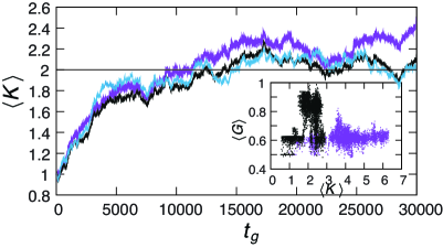
Figure 1: Convergence of the average network connectivity as a function of the GA generations $t_{g}$. FA task with $T=4$ and $N=100$. The curves are averaged over $30$ evolutionary runs (red), only the $22$ best (green), and the $15$ best (light blue) populations, respectively. Inset: scatter plot correlating average $\langle K\rangle(t_{g})$ and average generalization $\langle G\rangle(t_{g})$ of a successful population (black) and a suboptimal population (purple).

Interestingly, the population dynamics in our model follow Fisher’s fundamental theorem of natural selection, which attributes the rate of increase in the mean fitness to the increased fitness variance in the population edwards1994 . It has been shown in GAs that the diversity maximization Bedau94bifurcationstructure makes more configurations of the search space accessible to the genetic search to find optimal solutions carnevali87a ; carnevali87b ; patarnello89 .

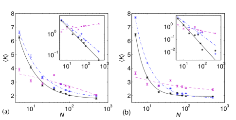
Figure 2: Finite size scaling of $\langle K\rangle$ as a function of $N$ for the three tasks, EO (black), FA (blue), R85 (magenta), and the training sample size $T=4$ (a) and $T=8$ (b). Points represent the data of the evolved networks, lines represent the fits. The finite size scaling for $\langle K\rangle$ shows that it scales with a power-law as a function of the system size $N$. The dashed lines represent the power-law fit of the form $a*x^{b}+c$. We favor the data for larger $N$ by weighting the data according to $N/N_{max}$, where $N_{max}=500$. The insets show $K_{c}-c$ as a function of $N$ on a log-log scale.

Indeed, we find that the standard deviation of the fitness values in the populations has a local maximum near $K_{c}$ (Fig. 4, inset), with a sharp decay toward larger $\langle K\rangle$, indicative of maximum diversity near criticality. Evidently, this diversity helps to maintain a high fitness population in the face of continuous mutations with a fairly high rate ($0.8$ in our study). While the average fitness can be lower (and often is), compared to less diverse populations, the probability to find and maintain high fitness solutions is strongly increased. Indeed, we find that populations where the best mutant has maximum fitness ($f=1$) sharply peak near $K_{c}$ (Fig. 4), as well as populations where the best mutant reaches perfect generalization. To find a possible source of fitness diversity, we determined several topological measures of the networks rubinov2010 : the eccentricity (maximum shortest path between a vertex $v$ and any other vertex in a graph), the betweenness centrality (the average fraction of shortest paths between all vertices in a graph that passes through a vertex $v$), the participation, and the characteristic path length. These measures were calculated for Erdös-Rényi (ER), eXponential Random Graphs (XRG), as well as for the evolved networks (Fig. 3). In fact, we find that the graph-theoretical measures have maximal variance near $K_{c}=2$. Similarly, other authors have shown that dynamical diversity is maximized near $K_{c}$, too Nykter2008 . Our results suggest that evolving RBN can indeed exploit this diversity to optimize learning.

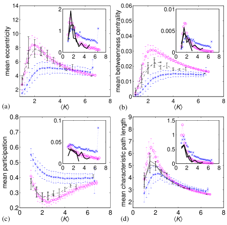
Figure 3: Near $K_{c}$, the topology of the network shows maximal variance. The insets show the standard deviation of the topological measures for initial ER networks (magenta), the evolved networks (black), and the XRG (blue). The solid lines represent the topological measures in random networks. The dotted line represents the same measure in RBNs.

In addition, we find that during the learning process of the networks, the in-degree distribution changes from a Poissonian to an exponential distribution. In particular, we observe that the topological properties of the networks reach a compromise between ER graphs and the XRG. The same observation was made in input- and output-less RBNs that were driven to criticality by using a local rewiring rule BornholRohlf00 . This significant topology change is related to diversity (entropy) maximization during the learning phase RevModPhys.80.1275 . However, this is beyond the scope of this paper and will be discussed in a separate publication.

Finally, we measured the damage spreading in the evolved RBNs DerridaP86 to determine their dynamical regime. The damage spreading $d_{t+1}$ is measured by changing the state of a randomly selected node in two identical networks. The two networks are simulated for a single time step and the damage spreading $\bar{d}$ is then calculated by averaging the ratio $\frac{d_{t+1}}{d_{t}}$ over many trails with random initial network configurations. One observes that for critical networks $\bar{d}=1$, for supercritical networks $\bar{d}>1$, and for subcritical networks $\bar{d}<1$. We see that for networks with a high fitness, $\bar{d}$ peaks around $1$ for all $N$.

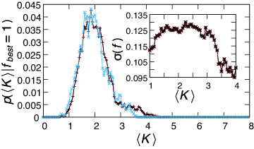
Figure 4: The conditional probability that evolving populations, where the best mutant reaches maximum fitness (i.e., $f_{best}=f_{max}=1$), have average connectivity $\langle K\rangle$ shows a sharp peak near $K_{c}$ (black curve), the same is found for maximum generalization (light blue). Inset: diversity of evolving populations, quantified in terms of the standard deviation $\sigma(f)$ of fitness distributions, has a maximum near $K_{c}=2$. All data sampled over the best $22$ out of $30$ populations for full-adder task with $T=4$ and $N=100$.

Discussion.— We investigated the learning and generalization capabilities in RBNs and showed that they evolve toward a critical connectivity of $K_{c}\approx 2$ for large networks and large input sample sizes. For finite size networks, the connectivity approaches the critical value with a power-law of the system size $N$. We showed that network learning and generalization are optimized near criticality, given task complexity and the amount of information provided surpass threshold values. Furthermore, critical RBN populations exhibit the largest diversity (variance) in fitness values, which supports learning and robustness of solutions under continuous mutations. By considering graph-theoretical measures, we determined that $K_{c}$ corresponds to a region in network ensemble space where the topological diversity is maximized, which may explain the observed diversity in critical populations.

Interestingly, we observe that RBN populations that are optimal with respect to learning and generalization tend to show average connectivity values slightly below $\langle K\rangle=2$. This may be related to previous results indicating that $K_{c}<2$ in finite size RBN RohlfGulbahceTeuscher2007 .

Examination of the attractors of the final population confirms that the computation happens as partitioning of the state-space into disjoint attractors krawitz2007 . During the evolution, the attractor landscape changes so that there are enough attractors to properly process the inputs. The entire task is encoded as a hyper cycle (i.e., a set of mutually reachable attractors) in the network dynamics. The input combinations play the role of a multi-valued switch that pushes the dynamics out of one attractor into the next along the hyper cycle. Emergence of the large attractor basins make the computation highly robust to perturbations in the node state while maintaining sensitivity to input signals. All networks in our final population converge to fixed-point or cyclic attractors.

To summarize, we solved a long-standing question and showed that learning of classification tasks and adaptation can drive RBNs to the “edge of chaos” Kauffman93 , where high-diversity populations are maintained and on-going adaptation and robustness are optimized. Our study may have important implications for determining the optimal topology of a much larger class of complex dynamical networks where adaptive information processing needs to be achieved efficiently, robustly, and with limited connectivity (i.e., resources). This has applications, e.g., in the area of neural networks, complex networks, and more specifically in the area of emerging molecular and nanoscale networks and computing devices, which are expected to be built in a bottom-up way from vast numbers of simple, densely arranged components that exhibit high failure rates, are relatively slow, and connected in an unstructured way.

Acknowledgments. This work was partly funded by NSF grant # 1028120. The first author is grateful for the fruitful discussions with Guy Feldman and Lukas Svec.

References

- (1) A. M. Turing. In Machine Intelligence, edited by B. Meltzer and D. Michie (Edinburgh University Press, Edinburgh, UK, 1969), 3–23.
- (2) S. A. Kauffman, J. Theor. Biol. 22, 437 (1969)
- (3) S. A. Kauffman, The Origins of Order: Self-Organization and Selection in Evolution ( Oxford University Press, New York, 1993).
- (4) S. Bornholdt, Biol. Chem. 382, 1289–1299 (2001)
- (5) B. Derrida and Y., Pomeau, Europhys. Lett., 1, 45–49 (1986).
- (6) R. Albert and A. L. Barabási, Phys. Rev. Lett. 84, 5660 (2000)
- (7) B. Samuelson and C. Troein, Phys. Rev. Lett. 90, 098701 (2003).
- (8) C. G. Langton, Physica D, 42, 12-37 (1990).
- (9) N. H. Packard, in Dynamic Patterns in Complex Systems,, ed. by J. A. S. Kelso, A. J. Mandell, and M. F. Shlesinger (World Scientific, Singapore, 1988), p. 293-301.
- (10) M. Mitchell, J. P. Crutchfield, and P. T. Hraber, Complex Systems, 7, 89-130 (1993).
- (11) J. Lizier, M. Prokopenko, and A. Zomaya, in Proc. Eleventh Int’l Conference on the Simulation and Synthesis of Living Systems (Alife XI), (MIT Press, Cambridge, 2008), p. 374-381.
- (12) S. A. Kauffman, J. Theor. Biol. 149, 4, 467-505 (1991).
- (13) S. Bornholdt and T. Rohlf, Phys. Rev. Lett. 84, 6114, (2000).
- (14) M. Liu and K. E. Bassler, Phys. Rev. E., 74, 4, 41910 (2006).
- (15) U. Bastola and G. Parisi, Physica D 115, 203 (1998).
- (16) A. Patarnello and P. Carnevali. Europhysics Lett., 4, 4, 503–508 (1987).
- (17) P. Carnevali and S. Patarnello. Europhysics Lett., 4, 10, 1199–1204 (1987).
- (18) S. Patarnello and P. Carnevali. In Neural Computing Architectures: The Design of Brain-Like Machines, edited by I. Aleksander (North Oxford Academic, London, 1989), p. 117.
- (19) C. Van den Broeck and R. Kawai. Phys. Rev. A, 42, 10, 6210–6218 (1990).
- (20) S. Wolfram, Rev. Mod. Phys. 55, 601-644 (1983).
- (21) M. Zwick, Kybernetes, 33, 5/6, 877-905 (2004).
- (22) A. W. F. Edwards, Biological Reviews, 69:443–474 (1994).
- (23) M. A. Bedau and A. Bahm, In Artificial Life IV: Proc. of the Int’l Workshop on the Synthesis and Simulation of Living Systems, ed. by Brooks and Maes (MIT Press, Bradford, 1994), p. 258–268.
- (24) M. Rubinov and O. Sporns, NeuroImage 52, 1059–69 (2010).
- (25) M. Nykter et al., Phys. Rev. Lett., 100, 058702, (2008).
- (26) S. N. Dorogovtsev, A. V. Goltsev, and J. F. F. Mendes, Rev. Mod. Phys., 80, 4, 1275–1335 (2008).
- (27) T. Rohlf, N. Gulbahce, and C. Teuscher, Phys. Rev. Lett., 99, 248701 (2007).
- (28) P. Krawitz and I. Shmulevich, Phys. Rev. Lett., 98, 158701 (2007).