Abstract

The Searchlight Scheduling Problem was first studied in 2D polygons, where the goal is for point guards in fixed positions to rotate searchlights to catch an evasive intruder. Here the problem is extended to 3D polyhedra, with the guards now boundary segments who rotate half-planes of illumination.

After carefully detailing the 3D model, several results are established. The first is a nearly direct extension of the planar one-way sweep strategy using what we call exhaustive guards, a generalization that succeeds despite there being no well-defined notion in 3D of planar “clockwise rotation”. Next follow two results: every polyhedron with $r>0$ reflex edges can be searched by at most $r^{2}$ suitably placed guards, whereas just $r$ guards suffice if the polyhedron is orthogonal. (Minimizing the number of guards to search a given polyhedron is easily seen to be NP-hard.) Finally we show that deciding whether a given set of guards has a successful search schedule is strongly NP-hard, and that deciding if a given target area is searchable at all is strongly PSPACE-hard, even for orthogonal polyhedra. A number of peripheral results are proved en route to these central theorems, and several open problems remain for future work.

1 Introduction

Previous work

The Searchlight Scheduling Problem (SSP) was first studied in [8] as a search problem in simple polygons, where some stationary guards are tasked to locate an evasive, moving intruder by hitting him with searchlights. Each guard carries a searchlight, modeled as a 1-dimensional ray that can be continuously rotated, while the intruder runs unpredictably and with unbounded speed, trying to avoid the searchlights. Since the guards cannot know the position of the intruder until they catch him in their lights, the movements of the searchlights must follow a fixed schedule, which should guarantee that the intruder is caught in finite time, regardless of the path he decides to take. The search takes place in a polygonal region, whose sides act as obstacles both for the intruder’s movements and for the guards’ searchlights. In a way, the polygonal boundary benefits the intruder, who can hide behind corners and avoid scanning searchlights. But it can also turn into a cul-de-sac, if the guards manage to force the intruder into an enclosed area from which he cannot escape.

Thus SSP is the problem of deciding if there exists a successful search schedule for a given finite set of guards in a given simple polygon. Figure 1 shows an instance of SSP with a successful schedule.

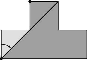
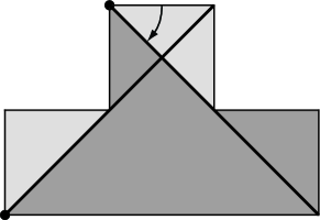
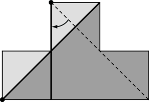
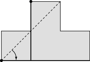
Figure 1: A search schedule for two guards in a polygon. At each stage, the dark area is still “contaminated”, the lighter areas have been cleared.

We will now briefly review some well-known results pertaining SSP in 2-dimensional polygons, before summarizing our results for the 3-dimensional model.

A trivial necessary condition for searchability is that the guard positions should guarantee that no point in the polygon is invisible to all guards. In other words, the guards should at least solve the Art Gallery Problem in the given polygon (see [6]), otherwise the intruder could sit at an uncovered point and never be discovered.

Another simple necessary condition is that every guard lying in the interior of the polygon (thus not on the boundary) should be visible to at least one other guard. Without this, the intruder could remain in a neighborhood of a guard and just avoid its rotating searchlight.

Several sufficient conditions for searchability are detailed in [8], all employing a general search algorithm called the one-way sweep strategy. Most notably, if all the guards lie on a simple polygon’s boundary and collectively see its whole interior, then they also have a successful search schedule.

Concerning the problem of minimizing the number of guards to search a given polygon, [8] contains a characterization of the simple polygons that are searchable by one or two suitably placed guards. A similar characterization for three guards was also found by the same authors, but never published ([10]). On the other hand, [11] contains some upper bounds on the minimum number of guards required to search a polygon (possibly with holes) as a function of the number of guards needed to solve the Art Gallery Problem in the same polygon.

The problem of determining the computational complexity of SSP was not directly addressed in [8], but has acquired more interest over time, and remains open. In [5] it is shown that SSP is solvable in double exponential time, by a discretization process that reduces the space of all possible searchlight schedules to a finite graph, which is then searched exhaustively. It is also straightforward to prove that SSP belongs to PSPACE$=$NPSPACE, because the information contained in a node can be stored efficiently, and the graph can be searched nondeterministically. It is still unknown whether SSP is NP-hard or even in NP. Conjecture 3.1 in [5] states that any searchable instance of SSP is also searchable by rotating each searchlight either exclusively clockwise or exclusively counterclockwise, from some initial position. Should this hold true, it would imply that SSP belongs at least to NP, but we can provide simple counterexamples, such as the one showed in Figure 2: either searchlight has to sweep back and forth, in order to search the polygon.

\psfrag{a}{$\ell_{1}$}\psfrag{b}{$\ell_{2}$}\includegraphics[width=125.74689pt]{fig02a.eps}

\psfrag{a}{$\ell_{1}$}\psfrag{b}{$\ell_{2}$}\includegraphics[width=125.74689pt]{fig02b.eps}

\psfrag{a}{$\ell_{1}$}\psfrag{b}{$\ell_{2}$}\includegraphics[width=125.74689pt]{fig02c.eps}

Figure 2: A searchable instance of SSP with no monotone search schedule. There are several search schedules (only one is depicted), but all of them rotate a searchlight back and forth.

In [9] the author (with M. Monge) extended the basic model to 3-dimensional polyhedra, as opposed to polygons. The traditional point guards then become segment guards, casting half-planes (as opposed to 1-dimensional rays), which can rotate with one degree of freedom. After providing some geometric motivations for the choice of the model and pointing out some of its basic features, the authors considered the optimization problem of searching a polyhedron in the shortest time, and proved its strong NP-hardness.

Our contribution

In this paper we further develop the theory of searching polyhedra by rotating half-planes: we expand on the results contained in [9] and we prove several new theorems. In Section 2 we give a careful and thorough definition of the model, which [9] lacked. In Section 3 we make preliminary observations and discuss the possibility of generalizing the main features of SSP to our model. Section 4 is devoted to algorithms to place guards in a given polyhedron that guarantee searchability, both for orthogonal and for general polyhedra. In Section 5 we show the strong NP-hardness of deciding if a polyhedron is searchable by a given set of guards, which greatly improves on the main result of [9]. Indeed, being able to minimize the search time (where infinite search time means unsearchable) allows a fortiori to decide searchability. We show also that deciding if a given target area is searchable (without necessarily searching the entire polyhedron) is strongly PSPACE-hard, even for orthogonal polyhedra. Section 6 contains concluding remarks and suggestions for further research.

2 Model definition

Polyhedra

For our purposes, a polyhedron will be the union of a finite set of closed tetrahedra (with mutually disjoint interiors) embedded in $\mathbb{R}^{3}$, whose boundary is a connected 2-manifold. As a consequence, a polyhedron is a compact topological space and its boundary is homeomorphic to a sphere or a $g$-torus. $g$ is also called the genus of the polyhedron, and by definition it is 0 if the polyhedron is homeomorphic to a ball. Moreover, the complement of a polyhedron with respect to $\mathbb{R}^{3}$ is connected. Since a polyhedron’s boundary is piecewise linear, the notion of face of a polyhedron is well-defined as a maximal planar subset of its boundary with connected and non-empty relative interior. Thus a face is a plane polygon, possibly with holes, and possibly with some degeneracies, such as hole boundaries touching each other at a single vertex. Any vertex of a face is also considered a vertex of the polyhedron. Edges are defined as minimal non-degenerate straight line segments shared by two faces and connecting two vertices of the polyhedron. Since a polyhedron’s boundary is an orientable 2-manifold, the relative interior of an edge lies on the boundary of exactly two faces, thus determining an internal dihedral angle (with respect to the polyhedron). A notch is an edge whose internal dihedral angle is reflex, i.e., strictly greater than $\pi$. Hence, convex polyhedra have no notches. A polyhedron is said to be orthogonal if each one of its edges is parallel to some axis.

Visibility with respect to a polyhedron $\mathcal{P}$ is a symmetric relation between points in $\mathbb{R}^{3}$: point $x$ sees point $y$ (equivalently, $y$ is visible to $x$) if the straight line segment joining $x$ with $y$ lies entirely in $\mathcal{P}$. Recall that $\mathcal{P}$ is a closed set, therefore such a segment could touch $\mathcal{P}$’s boundary, or even lie on it. When $\mathcal{P}$ is understood, we can safely omit any explicit reference to it.

Searchlight scheduling

Now we can state the problem-specific definitions. For simplicity, we consider only boundary guards, because they already yield a rich and diverse theory, unlike the situation in planar SSP.

Definition 1 (Guard).

A guard in a polyhedron $\mathcal{P}$ is a positive-length straight line segment without its endpoints, lying on the boundary of $\mathcal{P}$.

We exclude guard endpoints, because we don’t want them to see beyond notches or non-convex vertices, as the next definitions will clarify.

A guard is said to lie over edge $e$ if it coincides with the relative interior of $e$.

Definition 2 (Visibility region).

The visibility region $\mathcal{V}(\ell)$ of a guard $\ell$ in a polyhedron $\mathcal{P}$ is the set of points in $\mathcal{P}$ that are visible to at least one point in $\ell$.

Definition 3 (Searchplane).

A searchplane of a guard $\ell$ is the intersection between $\mathcal{V}(\ell)$ and any half-plane whose bounding line contains $\ell$.

Consequently, every guard has a searchplane for every possible direction of the half-plane generating it, and the union of a guard’s searchplanes coincides with its visibility region.

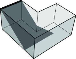
Figure 3: A guard and one of its searchplanes, depicted as a thick line and a dark surface, respectively.

If a searchplane is just a line segment, it’s said to be trivial, and the corresponding direction is said to be blind for its guard. We arbitrarily define a left and right side for each guard, and we call leftmost position the leftmost non-blind direction, for each guard. Similarly, we define the rightmost position of every guard. Observe that the leftmost and rightmost positions are well-defined, because the polyhedron is a closed set, and every direction aiming straight at its exterior is blind for a guard, even if the endpoints of (the topological closure of) the guard lie on reflex edges or vertices. This is because we didn’t include endpoints in Definition 1, a choice motivated also by Theorem 4. Conversely, every other direction is not blind, since the corresponding searchplanes must contain either some internal points of the polyhedron, or some points in the relative interior of a face.

Definition 4 (Schedule).

A schedule for a guard $\ell$ is a continuous function $f_{\ell}:[0,T]\to S^{1}$, where $T\in\mathbb{R}^{+}$ and $S^{1}$ is the unit circle.

Intuitively, $f_{\ell}(t)$ expresses the orientation of the guard at time $t\in[0,T]$, which is the angle at which $\ell$ is aiming its searchlight. In other words, $\ell$ is able to emit a half-plane of light in any desired direction, and to rotate it continuously about the axis defined by $\ell$ itself. We will say that, at time $t$, $\ell$ is aiming its searchlight at point $x$ if the orientation expressed by $f_{\ell}(t)$ corresponds to a searchplane of $\ell$ containing $x$ (assuming that one exists).

For the following definitions, we stipulate that a polyhedron $\mathcal{P}$ is given, along with a finite multiset of guards, each of which is provided with a schedule.

Definition 5 (Illuminated point).

A point is illuminated at a given time if some guard is aiming its searchlight at it.

Definition 6 (Contaminated point, clear point).

A point $x$ is contaminated at time $t$ if there exists a continuous function $g:[0,t]\to\mathcal{P}$ such that $g(t)=x$ and there is no time $t^{\prime}\in[0,t]$ at which $g(t^{\prime})$ is illuminated. A point that is not contaminated is said to be clear.

It follows that a maximal connected region of $\mathcal{P}$ without illuminated points is either all clear or all contaminated.

Definition 7 (Search schedule).

A set of schedules of the form $f_{\ell}:[0,T]\to S^{1}$, where $\ell$ ranges over a finite guard multiset in a polyhedron $\mathcal{P}$, is a search schedule if every point in $\mathcal{P}$ is clear at time $T$.

Next we define the 3-dimensional Searchlight Scheduling Problem (3SSP).

Definition 8 (3SSP).

3SSP is the problem of deciding if a given multiset of guards in a given polyhedron has a search schedule.

An instance of 3SSP is said to be searchable or unsearchable, depending on the existence of a search schedule for its guards.

Occasionally in our constructions we will need two guards to be coincident, hence we consider multisets of guards, as opposed to sets.

It is obvious, from these definitions, that 3SSP is not easier than SSP.

Proposition 1.

$\textsc{SSP}\leqslant_{\textsc{L}}\textsc{3SSP}$.

Proof.

Any polygon can be extruded to a prism, while each point guard can be transformed into a segment guard by stretching it parallel to the prism’s sides.∎

Notice, though, that not all reasonable models of 3-dimensional guards would yield such an immediate reduction.

Since an instance of 3SSP is trivially unsearchable if its guards can’t see the whole polyhedron, we want to exclude those instances.

Definition 9 (Viable instance).

An instance of 3SSP is viable if every point of the polyhedron belongs to the visibility region of at least one guard.

We will see that there are viable but unsearchable instances of 3SSP.

Finally, a relevant role is played by a special type of guard.

Definition 10 (Exhaustive searchplane).

A searchplane of a guard in a polyhedron $\mathcal{P}$ is exhaustive if it is a closed set whose relative boundary lies entirely on $\mathcal{P}$’s boundary.

Consider a guard $\ell$ with a non-trivial searchplane $S$, and let $\alpha$ be the plane containing $S$. Then $S$ is exhaustive if and only if it coincides with the connected component of $\alpha\cap\mathcal{P}$ containing $\ell$. Notice that the searchplane depicted in Figure 3 is not exhaustive, because one of its edges lies in the interior of the polyhedron (plus, it’s not a closed set: recall that guards have no endpoints).

Definition 11 (Exhaustive guard).

A guard is exhaustive if all its searchplanes are exhaustive.

Intuitively, an exhaustive guard is similar to a traditional boundary guard from SSP in simple polygons, in that its searchlight provides at any time an effective barrier which cannot be crossed by the intruder just by walking past its borders. The importance of such guards in developing search algorithms will be clear shortly.

3 Basic results

Counterexamples

The most noteworthy aspect of our guard model is that searchplanes, as opposed to searchlight rays emanating from boundary guards in SSP, may fail to disconnect a polyhedron when aimed at its interior, regardless of its genus. As it turns out, this is the main reason why 3SSP seems harder than SSP, in that exploiting such a property will enable the relatively simple NP-hardness proof in Section 5, as well as the construction of several counterexamples to positive statements about SSP.

For example, the reduction of the search space to sequential schedules (i.e., schedules in which the guards sweep in turns) given in [5] is no longer possible. Figure 4 shows an instance of 3SSP whose two guards are forced to turn their searchlights simultaneously, or else they would create gaps in the illuminated surface which would result in the recontamination of the whole polyhedron.

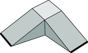
Figure 4: A searchable instance of 3SSP with no sequential search schedule. Thick lines mark guards.

Moreover, in spite of the searchability of all SSP instances whose guards lie on the boundary and collectively see the whole polygon (see [8]), it is easy to construct viable but unsearchable instances of 3SSP, such as those in Figure 5. Indeed, whenever the two guards attempt to clear the center (in either of these two instances), they fail to disconnect the polyhedron, since their searchplanes are not coplanar, which results in the recontamination of the entire instance. In Section 5 we will provide more sophisticated unsearchable but viable instances of 3SSP.

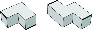
Figure 5: Two unsearchable instances of 3SSP whose guards solve the Art Gallery Problem.

Exhaustive guards

Notice that all the previous counterexamples employ guards that are not exhaustive. Conversely, it comes as no surprise that employing only exhaustive guards yields positive results. To see why, let’s give a characterization of the different shapes a searchplane can take with respect to the surrounding polyhedral environment. The topological closure of a searchplane is always a polygon, perhaps with holes, perhaps with some additional segments sticking out radially, and the whole searchplane is visible to some line segment lying on its external boundary, which would be the guard emanating it (refer to Figure 6). There may be intersections between a searchplane’s relative interior and the polyhedral boundary, which could be collections of polygons, straight line segments, and isolated points. But what’s central for our purposes is the searchplane’s relative boundary, which may entirely lie on the polyhedron’s boundary, or may not. If it does, and the searchplane is a closed set, then the only way an intruder could travel from one side of the searchplane to the other, without crossing the light and being caught, would be to take a detour through a suitable handle of the polyhedron. In particular, in 0-genus polyhedra, that would be impossible. In other words, any exhaustive guard aiming its searchlight at the interior of a 0-genus polyhedron, disconnects it.

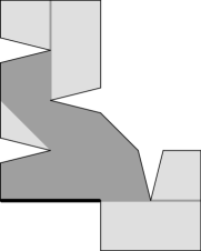
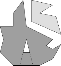
Figure 6: Two sections of polyhedra, with searchplanes represented as dark regions. The searchplane in 6 has two dangling segments, while the searchplane in 6 is exhaustive but not simply connected.

On the other hand, if $\ell\subset\mathcal{P}$ is exhaustive, the topological closure of $\mathcal{V}(\ell)$ is always a polyhedron, perhaps with some dangling polygons. Of course, the boundary of $\mathcal{V}(\ell)$ may contain polygons that do not lie on $\mathcal{P}$’s boundary. But, because $\ell$ is exhaustive, every such polygon is entirely contained in some searchplane of $\ell$, and the corresponding searchlight position will be called critical for $\ell$. Every exhaustive guard has only a finite number of critical positions.

Now, as an exhaustive guard $\ell$ in a 0-genus polyhedron starts turning from its leftmost position toward the right, every point that it illuminates will remain clear forever, unless the illuminated searchplane becomes tangent to some region of the polyhedron which is not in $\mathcal{V}(\ell)$ and which would be responsible for recontamination, once the tangency is crossed by the searchlight. This happens exactly when $\ell$ reaches a critical position.

One-way sweeping

We now have the tools required to generalize the one-way sweep strategy for guards in simple polygons (see [8]) to work with exhaustive guards in simply connected polyhedra.

Theorem 2.

Every viable 0-genus instance of 3SSP whose guards are exhaustive is searchable.

Proof.

We first sketch a search schedule before detailing it further. Select any guard $\ell$ and start turning it rightward from its leftmost position. As soon as it reaches a critical position, it means that some subpolyhedron $\mathcal{R}\subset\mathcal{P}$ has been encountered that is invisible to $\ell$. So stop turning $\ell$ and select another guard to continue the job. Proceed recursively until $\mathcal{R}$ is clear, then turn $\ell$ rightward again, stopping at every critical position, until the entire polyhedron is clear.

At any time, there is a clear region of $\mathcal{P}$ that is steadily growing, and a semiconvex subpolyhedron $\mathcal{R}$ supported by a set of guards $L$ that is being cleared by some guard not in $L$, while the guards in $L$ hold their searchlights fixed. Intuitively, the term “semiconvex” is used because the only points of non-convexity of such a polyhedron lie on $\mathcal{P}$’s boundary. For a formal definition of semiconvex subpolygon and support, refer to [8] or [5]. Extending these definitions to polyhedra is straightforward, since we’re considering only exhaustive guards in 0-genus polyhedra. Thus, part of the boundary of $\mathcal{R}$ coincides with $\mathcal{P}$’s boundary, while the remaining part is determined by the searchplanes of the guards in $L$. Moreover, all the guards in $L$ are in a critical position, waiting for $\mathcal{R}$ (or some larger semiconvex subpolyhedron of $\mathcal{P}$, supported by a subset of $L$) to be cleared. It follows that none of the guards in $L$ can see any point in the interior of $\mathcal{R}$.

Hence, there must be some guards not in $L$ that can see an internal portion of $\mathcal{R}$, otherwise the problem instance wouldn’t be viable. We select one of them, say $\ell^{\prime}$, and start sweeping $\mathcal{R}$ from left to right. Notice that a searchplane bounding $\mathcal{R}$ could have holes, and thus $\mathcal{R}$ itself could have strictly positive genus. But that does not affect our invariants, because every searchplane of $\ell^{\prime}$ passing through $\mathcal{R}$’s interior still disconnects it, or it wouldn’t even disconnect $\mathcal{P}$. As a consequence, the points in $\mathcal{R}$ that are illuminated by $\ell^{\prime}$ never get recontaminated as $\ell^{\prime}$ continues its sweep.

Again, whenever $\ell^{\prime}$ reaches a critical position, it stops there until the semiconvex subpolyhedron $\mathcal{R}^{\prime}\subset\mathcal{R}$ supported by $L\cup\{\ell^{\prime}\}$ has been cleared by some other guard, and so on recursively. Since every guard has only a finite number of critical positions, eventually $\mathcal{P}$ gets cleared.∎

Remarkably enough, the core argument supporting the planar one-way sweep strategy of [8] applies also to our polyhedral model, where there is no well-defined global concept of clockwise rotation.

Sequentiality

In addition to this, a version of the main result of [5] also extends to instances of 3SSP with exhaustive guards. We say that a search schedule is critical and sequential if at most one guard is turning at any given time, and guards stop or change direction only at critical positions, or at their leftmost or rightmost positions.

Corollary 3.

Every searchable 0-genus instance of 3SSP whose guards are exhaustive has a critical and sequential search schedule.

Proof.

Since the instance is searchable, it must be viable. Thus, the search schedule detailed in the proof of Theorem 2 applies, which is indeed critical and sequential.∎

Searching with one guard

As a further application of the concept of exhaustive guard, we characterize the searchable instances of 3SSP having just one guard, which turn out to be all the viable ones.

Theorem 4.

Every viable instance of 3SSP with just one guard is searchable.

Proof.

Since the instance is viable, the visibility region of its only guard $\ell$ coincides with the whole polyhedron $\mathcal{P}$. Let $\ell^{\prime}$ be the maximal straight line segment contained in $\mathcal{P}$ and containing $\ell$. Then $\ell^{\prime}$ entirely belongs to the boundary of $\mathcal{P}$. Indeed, if a point $x\in\ell^{\prime}$ lay strictly in the interior of $\mathcal{P}$, then also some neighborhood of $x$ would. Recall that $\ell$ has a range of blind directions past its leftmost and rightmost position, where all its searchplanes degenerate to the single line $\ell^{\prime}$. In all those directions, part of the neighborhood of $x$ would lie outside $\mathcal{V}(\ell)$, contradicting the viability of the instance.

\psfrag{a}{$\alpha$}\psfrag{x}{$x$}\psfrag{s}{$S$}\psfrag{l}{$\ell$}\psfrag{j}{$\ell^{\prime}$}\includegraphics[scale={0.5}]{fignew1.eps}

Figure 7: An illustration of the proof of Theorem 4.

Consider a searchplane $S$, lying on a half-plane $\alpha$ whose bounding line contains $\ell$ (refer to Figure 7). If a point $x\in\alpha\cap\mathcal{P}$ lay outside $S$, then $x$ would necessarily be covered by another searchplane, because $\mathcal{V}(\ell)=\mathcal{P}$. But the only points in $\alpha$ that could lie on a searchplane different from $S$ would be those in $\ell^{\prime}$, because any two searchplanes of $\ell$ intersect just on $\ell^{\prime}$. Nonetheless, $\ell^{\prime}$ belongs to $S$ too, which yields a contradiction. Hence $S=\alpha\cap\mathcal{P}$ and also $\ell^{\prime}$ lies on the boundary of $\mathcal{P}$, implying that $\ell$ is an exhaustive guard with no critical positions. Moreover, $S$ disconnects $\mathcal{P}$ if it intersects its interior. Suppose by contradiction that an intruder could walk from one side of $S$ to the other side. Since $S=\alpha\cap\mathcal{P}$, the intruder would necessarily have to take the long route around $\ell^{\prime}$ (i.e., opposite to $\alpha$, see Figure 7), and by doing so it would cross all the half-planes in the blind directions of $\ell$. But the only points of $\mathcal{P}$ that belong to such half-planes are those in $\ell^{\prime}$, so the intruder would be caught in any case.

It follows that turning $\ell$ from its leftmost position to its rightmost position produces a search schedule.∎

Notice that the above characterization includes polyhedra of any genus, not just 0. Also notice that, had we included endpoints in Definition 1, the statement of Theorem 4 would have been false. Indeed, the viability assumption would have been satisfied by more 3SSP instances, including unsearchable ones (such as a cube with a “pyramidal well” pointing inside, and a guard over a notch).

Checking exhaustiveness

We conclude this Section by sketching an argument supporting the claim that the conditions of Theorem 2 are practically checkable.

Proposition 5.

The exhaustiveness of a guard $\ell\subset\mathcal{P}$ can be decided in time polynomial in the size of $\mathcal{P}$.

Proof.

First of all, the exhaustiveness of a searchplane $S$ generated by a half-plane $\alpha$ can be efficiently checked by computing the polygonal section $P=\alpha\cap\mathcal{P}$, and then computing the boundary of $S$ by drawing lines through every pair of vertices of $P$. Once the boundary of $S$ is known, its exhaustiveness can be checked easily.

Now, determining if $\ell$ is exhaustive can be carried out by inspecting just a polynomial number of its searchplanes. For every face $F\subset\mathcal{P}$ and every non-parallel edge $e\subset\mathcal{P}$, we call the point of intersection between the plane containing $F$ and the line containing $e$ an event. In particular, every vertex of $\mathcal{P}$ is an event. Imagine turning the searchlight of $\ell$ from its leftmost position to the rightmost: it is straightforward to see that the exhaustiveness of the illuminated searchplane can change only when the searchlight crosses an event. Hence, it suffices to check the exhaustiveness of every searchplane corresponding to an event, plus one searchplane for each interval between two consecutive events. The number of searchplanes to check is thus polynomial.∎

4 Search strategies

In this Section we attempt to solve the problem of efficiently placing guards in a given polyhedron in order to make it searchable, while partially settling Conjecture 1 in [9] (i.e., that any polyhedron with a guard over each notch is searchable). Our general approach employs $r^{2}$ guards for polyhedra with $r>0$ notches, which we believe to be asymptotically suboptimal. However, we also prove that just $r$ guards are sufficient for orthogonal polyhedra. A related goal is to minimize the search time, which is the total time of a search schedule, assuming that the maximum angular speed of every guard is $2\pi~{}\mathrm{rad}/\mathrm{sec}$ (i.e., the set of its legal schedules is restricted to Lipschitz continuous functions, whose Lipschitz constants match an angular speed of $2\pi~{}\mathrm{rad}/\mathrm{sec}$). We will show that occasionally it is possible to trade guards for search speed, to some extent.

Minimizing guards

The problem of minimizing the number of guards required to search a given polyhedron is strongly NP-hard, even for 0-genus orthogonal polyhedra. The problem is strongly NP-hard also if the guards are required to lie over edges, or just over notches. Indeed, the same approach used in [3] to show the strong NP-hardness of the Art Gallery Problem with vertex guards in general polygons can be employed, with some additional adjustments, to construct a simple orthogonal polygon with the same properties. By subsequently extruding the polygon into an orthogonal prism and after some minor modifications, the same hardness result can be obtained for edge guards, as well. Finally, passing from the Art Gallery Problem to 3SSP is almost automatic because, as proved in [8], boundary point guards can search a simple polygon if and only if they solve the Art Gallery Problem.

4.1 Searching general polyhedra

Open edge guarding

We first need to consider a planar Art Gallery Problem for open edge guards (i.e., edge guards without endpoints), which has apparently not been previously explored. Specifically, we want to select some edges of a given polygon $P$, in such a way that each point of $P$ is visible to an internal point of at least one of the selected edges. For technical reasons (see the proof of Theorem 6), we also want to force the selection of a specific edge.

Lemma 1.

Every polygon with $r$ reflex vertices, $h$ holes and a distinguished edge $e$ is guardable by at most $r-h+1$ open edge guards, one of which lies over $e$.

Proof.

Let $P$ be a polygon, select any reflex vertex $v$ and draw the bisector of the corresponding internal angle, until it again hits the boundary of $P$. If the ray hits another vertex, slightly rotate it about $v$, so that it instead hits the interior of an edge. Two situations can occur: either $P$ gets partitioned in two parts, with $r-1$ total reflex vertices and $h$ total holes, or two connected components of the boundary are joined, so that $P$ loses both a hole and a reflex vertex.

\psfrag{e}{$e$}\includegraphics[scale={0.35}]{fig07a.eps}

\psfrag{e}{$e$}\includegraphics[scale={0.35}]{fig07b.eps}

Figure 8: An example of the construction in Lemma 1. In 8 the first step is shown, where the dotted line acts as a degenerate edge of the resulting polygon. In 8 the final partition is shown, with the selected edges represented as thick lines.

Repeat the process inductively on the resulting polygons, until no reflex vertex remains. Notice that polygonal boundaries may be degenerate in the intermediate steps of this construction, meaning that a single segment should occasionally be regarded as two coincident segments (refer to Figure 8). $P$ is now partitioned into convex pieces, which of course have no holes. Thus, during the process, the number of holes decreased $h$ times, while the number of pieces in the partition increased $r-h$ times, resulting in $r-h+1$ convex polygons. Additionally, each polygon has at least one edge lying on $P$’s boundary, and conversely every internal point of each edge of $P$ sees at least one complete region. Place a guard on $e$, thus guarding at least one region of the partition. For each unguarded (or partially guarded) region, choose an edge of $P$ that completely sees it, and place a guard on it. As a result, $P$ is completely guarded and at most $r-h+1$ open edge guards have been placed.∎

The previous bound is asymptotically best possible, because polygons with $r$ reflex vertices can be constructed which require $r$ open edge guards, for every $r$.

Search strategy

Theorem 6.

Any polyhedron with $r>0$ notches can be searched by at most $r^{2}$ suitably placed guards.

Proof.

Let $\mathcal{P}$ be a non-convex polyhedron. We first partition it into convex regions by placing at most $r^{2}$ guards, then we show that some guards can be turned in a certain order to clear every piece of the partition.

First partition.

Let $e$ be a notch of $\mathcal{P}$, and let $\alpha_{e}$ be a plane through $e$, close enough to its angle bisector, but not containing any vertex of $\mathcal{P}$ other than $e$’s endpoints. Let $\mathcal{Q}_{e}$ be the connected component of $\mathcal{\alpha}_{e}\cap\mathcal{P}$ containing $e$. We claim that $\mathcal{Q}_{e}$ is a polygon with at most $r-1$ reflex vertices, possibly with holes. Indeed, $e$ is an edge of $\mathcal{Q}_{e}$, and each reflex vertex of $\mathcal{Q}_{e}$ lies on a notch of $\mathcal{P}$. Moreover, if an endpoint of $e$ is a reflex vertex of $\mathcal{Q}_{e}$, then it belongs at least to another notch of $\mathcal{P}$, different from $e$. But $\alpha_{e}$ intersects every edge of $\mathcal{P}$ other than $e$ in at most one point (otherwise it would contain its endpoints, as well), hence there are at most $r-1$ reflex vertices of $\mathcal{Q}_{e}$, i.e., one for every notch of $\mathcal{P}$ other than $e$.

By Lemma 1, $\mathcal{Q}_{e}$ can be guarded by at most $r$ (2-dimensional) open edge guards, one of which lies over $e$. Equivalently, $\mathcal{Q}_{e}$ can be completely illuminated by at most $r$ suitably placed guards (with searchlights), lying on $\alpha_{e}$ and aimed parallel to it, one of which lies over $e$. By repeating the same construction with every other notch, at most $r^{2}$ guards are placed, and $\mathcal{P}$ is partitioned by illuminated searchplanes into convex polyhedra $\mathcal{C}_{i}$. We remark that, during our construction, previously placed searchplanes are not considered as part of $\mathcal{P}$’s boundary. Hence, every $\mathcal{Q}_{e_{k}}$ is indeed bounded by $\mathcal{P}$. This is because we need to place guards on the boundary of $\mathcal{P}$, and not in its interior.

(A very similar partition technique can be found in [1], under the name of “naive decomposition”.)

A coarser partition.

Consider now a slightly different partition: proceed as above by drawing angle bisectors through notches, but this time every previously drawn splitting polygon acts as a boundary. In other words, as soon as $\mathcal{P}$ splits into several subpolyhedra, we partition them recursively one by one, confining each split to just one subpolyhedron. So, if we consider some intermediate subpolyhedron $\mathcal{P}^{\prime}\subseteq\mathcal{P}$ and select a notch $e^{\prime}\subset\mathcal{P}^{\prime}$, we look at the notch $e$ of $\mathcal{P}$ that contains $e^{\prime}$, and let $\mathcal{R}_{e^{\prime}}$ be the connected component of $\alpha_{e}\cap\mathcal{P}^{\prime}$ (as opposed to $\alpha_{e}\cap\mathcal{P}$) containing $e^{\prime}$. As a result, $\mathcal{P}$ is again partitioned into convex polyhedra $\mathcal{D}_{j}$, in such a way that every $\mathcal{C}_{i}$ is contained in some $\mathcal{D}_{j}$ (i.e., $\{\mathcal{C}_{i}\}$ is a refinement of $\{\mathcal{D}_{j}\}$). Notice that, even though two different splitting polygons $\mathcal{R}_{e^{\prime}}$ and $\mathcal{R}_{e^{\prime\prime}}$ may correspond to the same notch $e$ of $\mathcal{P}$ (because $e$ itself has been split by a previous cut), they are nonetheless coplanar, as they both belong to the same plane $\alpha_{e}$.

(a) $\{\mathcal{C}_{i}\}$

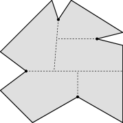
(b) $\{\mathcal{D}_{j}\}$

Figure 9: A comparison of the partitions $\{\mathcal{C}_{i}\}$ and $\{\mathcal{D}_{j}\}$ in a section of a polyhedron. For simplicity, only the splitting planes corresponding to visible notches are shown.

Partition tree.

The point of having this coarser partition is that every $\mathcal{D}_{j}$ contains a subsegment of a notch of $\mathcal{P}$ (see Figure 9). This property can be checked by a straightforward induction on the construction steps. More specifically, we build a tree during the splitting process, whose nodes represent the intermediate subpolyhedra, and whose arcs are marked by the splitting polygons $\mathcal{R}_{e}$ (see Figure 10). Thus, the root of the tree is $\mathcal{P}$ and its leaves are the $\mathcal{D}_{j}$’s. Every time we draw a splitting polygon $\mathcal{R}_{e}$ for a subpolyhedron $\mathcal{P}^{\prime}$ corresponding to some node $v$ of the tree, we could either decrease the genus of $\mathcal{P}^{\prime}$, or we could partition it into two subpolyhedra $\mathcal{P}^{\prime}_{1}$ and $\mathcal{P}^{\prime}_{2}$, one for each side of $\mathcal{R}_{e}$. In the first case we just attach to $v$ an arc labeled $\mathcal{R}_{e}$ with a node labeled as the new polyhedron, say $\mathcal{P}^{\prime\prime}$. In the second case we attach to $v$ two arcs labeled $\mathcal{R}_{e}$, with two sibling nodes labeled $\mathcal{P}^{\prime}_{1}$ and $\mathcal{P}^{\prime}_{2}$. This structure is somewhat reminiscent of a Binary Space Partitioning tree. Again, like in the proof of Lemma 1, we have to slightly extend the notion of polyhedron, to include those with internal polygons acting as faces, resulting from non-disconnecting splits.

\psfrag{a}{$\mathcal{P}$}\psfrag{b}{$\mathcal{P}_{1}$}\psfrag{c}{$\mathcal{P}_{2}$}\psfrag{d}{$\mathcal{P}_{1}^{\prime}$}\psfrag{e}{$\mathcal{P}_{2}^{\prime}$}\psfrag{f}{$\mathcal{P}_{2}^{\prime\prime}$}\psfrag{g}{$\mathcal{D}_{1}$}\psfrag{h}{$\mathcal{D}_{2}$}\psfrag{i}{$\mathcal{D}_{3}$}\psfrag{j}{${}_{\mathcal{R}_{e_{1}}}$}\psfrag{k}{${}_{\mathcal{R}_{e_{2}}}$}\psfrag{l}{${}_{\mathcal{R}_{e_{3}}}$}\includegraphics[scale={1.1}]{fignew3.eps}

Figure 10: A sketch of a partition tree.

Search schedule.

Next we describe a search schedule for the $r^{2}$ guards we placed. We turn only some of the $r$ guards that lie over the notches of $\mathcal{P}$, one by one, while all the other guards stay still. The order of activation of the guards is determined by the above partition tree, and the same guard could be activated more than once. The subpolyhedra of $\mathcal{P}$ are cleared recursively by a depth-first walk of the partition tree, starting from the root. Every time a leaf is reached through an arc labeled $\mathcal{R}_{e}$, its corresponding $\mathcal{D}_{j}$ is swept by the guard lying on $e$. This is feasible because $e$ lies on the boundary of $\mathcal{D}_{j}$, which is convex. After $\mathcal{D}_{j}$ is clear, the guard moves back to its initial position and the depth-first walk proceeds.

Correctness.

It remains to show that no significant recontamination can occur among the $\mathcal{D}_{j}$’s while their bounding searchlights are rotated. Suppose the depth-first walk reaches a leaf of the tree labeled $\mathcal{D}_{j}$, and let $\ell_{e}$ be the guard whose duty is to clear $\mathcal{D}_{j}$. Perhaps the corresponding edge $e$ of $\mathcal{P}$ is divided several times by the partition, so let $E$ be the set of subsegments of $e$ whose corresponding splitting planes actually appear as labels of the edges of the partition tree. Let $e^{\prime}\in E$ be the subsegment of $e$ that is also an edge of $\mathcal{D}_{j}$. On the other side of $\mathcal{R}_{e^{\prime}}$ lies a subpolyhedron $\mathcal{P}^{\prime}$, such that $\mathcal{D}_{j}$ and $\mathcal{P}^{\prime}$ are represented by sibling nodes in the partition tree. In order to clear $\mathcal{D}_{j}$, $\ell_{e}$ turns its searchlight from $\mathcal{R}_{e^{\prime}}$ to sweep over $\mathcal{D}_{j}$, and then back to $\mathcal{R}_{e^{\prime}}$. Since the restriction of $\ell_{e}$ to $\mathcal{D}_{j}$ is exhaustive, no recontamination occurs between $\mathcal{D}_{j}$ and $\mathcal{P}^{\prime}$ during this back-and-forth sweep (see Figure 11).

\psfrag{e}{$\ell_{e}$}\psfrag{r}{${}_{\mathcal{R}_{e^{\prime}}}$}\psfrag{d}{$\mathcal{D}_{j}$}\psfrag{p}{$\mathcal{P}^{\prime}$}\includegraphics[scale={0.6}]{fig08.eps}

Figure 11: $\mathcal{P}^{\prime}$ is not recontaminated while $\ell_{e}$ sweeps $\mathcal{D}_{j}$.

Nonetheless, recontamination could still occur between other subpolyhedra bounded by $\alpha_{e}$. Let $\{e_{1},e_{2}\}\subseteq E$, and let the subpolyhedra $\mathcal{P}_{1}$ and $\mathcal{P}_{2}$ be partitioned by $\mathcal{R}_{e_{1}}$, and $\mathcal{R}_{e_{2}}$, respectively (observe that the relative interiors of $e_{1}$ and $e_{2}$ must be disjoint, by construction). Obviously, no recontamination between $\mathcal{P}_{1}$ and $\mathcal{P}_{2}$ is possible while $\ell_{e}$ sweeps, because $\alpha_{e}$ is not a common boundary (refer to Figure 12). However, recontamination could occur within $\mathcal{P}_{1}$ (or within $\mathcal{P}_{2}$), provided that $e_{1}\neq e^{\prime}$. As it turns out, this type of recontamination is irrelevant, because it would imply that the node labeled $\mathcal{P}_{1}$ (call it $p$) has not been reached yet by the depth-first walk in the partition tree. We set up an induction argument on the partition tree, assuming that all the subpolyhedra corresponding to previously visited leaves are still clear before $\ell_{e}$ sweeps. By construction, $p$ cannot be an ancestor of the node labeled $\mathcal{D}_{j}$, otherwise $\mathcal{D}_{j}$ would be a subpolyhedron of $\mathcal{P}_{1}$, while in fact their interiors are disjoint. So, had the depth-first walk reached $p$, it would have also visited its entire dangling subtree and, by inductive assumption, $\mathcal{P}_{1}$ would still be all clear. Moreover, since $\mathcal{P}_{1}$ is not bounded by $\alpha_{e}$, it cannot get recontaminated while $\ell_{e}$ sweeps. On the other hand, if the walk has not reached $p$ yet, then perhaps some portions of $\mathcal{P}_{1}$ have been accidentally cleared, but can safely be recontaminated, because the systematic clearing process of $\mathcal{P}_{1}$ has yet to start.∎

\psfrag{a}{$\alpha_{e}$}\psfrag{b}{$\mathcal{R}_{e_{1}}$}\psfrag{c}{$\mathcal{R}_{e_{2}}$}\psfrag{d}{$\mathcal{R}_{e^{\prime}}$}\psfrag{e}{$e$}\psfrag{f}{$e_{1}$}\psfrag{g}{$e_{2}$}\psfrag{h}{$e^{\prime}$}\psfrag{p}{$\mathcal{P}_{1}$}\psfrag{q}{$\mathcal{P}_{2}$}\psfrag{r}{$\mathcal{P}^{\prime}$}\psfrag{s}{$\mathcal{D}_{j}$}\includegraphics[scale={0.9}]{fignew4.eps}

Figure 12: A sketch of a splitting plane.

Improving search time

The search time of our schedule could be quadratic in $r$, but we can trivially achieve constant search time by placing $r$ additional guards.

Corollary 7.

Any polyhedron with $r>0$ notches can be searched in less than 1 second by at most $r^{2}+r$ suitably placed guards.

Proof.

Place $r^{2}$ guards as in the proof of Theorem 6 and never move them, so that the partition $\{\mathcal{D}_{j}\}$ is always preserved. Then add a guard over every notch, and turn these additional guards simultaneously, from their leftmost position to the rightmost. Every guard turns by less than $2\pi~{}\mathrm{rad}$, so the search time is less than 1 second.∎

4.2 Searching orthogonal polyhedra

The previous result can be greatly improved if the polyhedron is orthogonal.

We define the vertical direction (or up-down direction) as the direction parallel to the $z$-axis. Accordingly, any direction parallel to the $xy$-plane is called horizontal, and the direction parallel to the $x$-axis (resp. $y$-axis) is called left-right (resp. front-back) direction. Thus, the edges and faces of any orthogonal polyhedron are either vertical or horizontal, and the $x$-orthogonal (resp. $y$-orthogonal) faces are called lateral faces (resp. front faces).

Erecting fences

We first construct a partition of a given orthogonal polyhedron $\mathcal{P}$ into cuboids (i.e., rectangular boxes) by a 3-step process.

1. Each horizontal notch $r$ of $\mathcal{P}$ has a horizontal adjacent face and a vertical adjacent face $F$, going upwards or downwards. From every point on $r$, send a vertical ray in the direction opposite to $F$, until it again reaches the boundary of $\mathcal{P}$. Repeat the process with every horizontal notch, so that each generates a vertical fence, either upwards or downwards. It’s easy to see that $\mathcal{P}$ is partitioned by fences into orthogonal prisms (i.e., extruded polygons) with horizontal bases.

2. Consider a vertical notch $r$ of $\mathcal{P}$ with an internal point lying on a lateral face of a prism $\mathcal{Q}$ generated in Step 1. By construction, $r$ must lie entirely on the boundary of $\mathcal{Q}$. Extend $r$ to a maximal segment $r^{\prime}$ contained in the boundary of $\mathcal{Q}$. If possible, send a horizontal ray from every point of $r^{\prime}$, going through the interior of $\mathcal{Q}$ in the left-right direction, until it reaches $\mathcal{Q}$’s boundary, as shown in Figure 13. Do the same with every vertical notch of $\mathcal{P}$ lying on a lateral face of some prism, so that the initial partition gets further refined by these new fences. Clearly, to every such notch corresponds just one fence, which in turn goes through the interior of just one prism.

   \psfrag{r}{$r$}\psfrag{s}{$r^{\prime}$}\psfrag{q}{$\mathcal{Q}$}\includegraphics[scale={0.7}]{fignew5.eps}

   Figure 13: A fence generated by $r$ during Step 2. Fences are shown as darker regions.

3. The pieces resulting from Step 2 are once again prisms, perhaps with some additional non-disconnecting vertical fences. By construction, each reflex edge of such a prism is vertical, with no edges of $\mathcal{P}$ lying on it. Repeat the procedure in Step 2 also with these reflex edges, sending horizontal rays and thus building vertical fences which extend laterally the front faces of the prisms, as shown in Figure 14. As a result, $\mathcal{P}$ gets partitioned into cuboids.

(The term “fence” is borrowed from [2]).

\psfrag{l}{$\ell$}\psfrag{f}{$F$}\psfrag{g}{$F^{\prime}$}\psfrag{r}{$r$}\psfrag{x}{$x$}\psfrag{c}{$\mathcal{C}$}\psfrag{d}{$\mathcal{C}^{\prime}$}\includegraphics[scale={1}]{fig09.eps}

Figure 14: A fence generated by $r$ during Step 3. Fences are shown as darker regions. The nomenclature comes from Lemmas 2 and 3.

Placing guards

Now place a guard over every notch of $\mathcal{P}$. Aim horizontal guards vertically and aim vertical guards in the left-right direction, in such a way that every guard aims at the interior of $\mathcal{P}$. We first want to prove that the fences in our 3-step construction are coherent with searchlights.

Lemma 2.

Every fence is contained in some illuminated searchplane.

Proof.

The claim is obvious for fences constructed in Step 1 and Step 2. As for fences constructed in Step 3, consider an edge $r$ generating one of them (see Figure 14). Recall that $r$ is a reflex edge of a prism, let it be $\mathcal{Q}$, in the partition obtained in Step 1. By the construction in Step 2, $r$ contains no notch of $\mathcal{P}$. Hence its adjacent front face $F\subset\mathcal{Q}$ has no intersection with the boundary of $\mathcal{P}$, at least in a neighborhood of $r$. But the bases of $\mathcal{Q}$ belong to the boundary of $\mathcal{P}$, because no horizontal fences were constructed. Then, at least a subsegment of a horizontal edge of $F$, sharing an endpoint with $r$, belongs to a notch of $\mathcal{P}$, and hence belongs to a guard $\ell$. As a consequence, $\ell$ illuminates the whole fence generated by $r$ in Step 3.∎

Thus, every fence belongs to one guard. We could also incorporate each fence built in Step 3 into its adjacent vertical fence built in Step 1, which belongs to the same guard. As a result, every guard generates at most one fence.

Lemma 3.

Every cuboid in the partition belongs entirely to the visibility region of any guard whose fence bounds it.

Proof.

If a fence built in Step 1 bounds a cuboid, then it belongs to a guard $\ell$ located, at least partially, on its border. Indeed, fences are vertical and the upper and lower faces of a cuboid belong to faces of $\mathcal{P}$, and therefore $\ell$ cannot lie entirely outside the cuboid. It follows that $\ell$ sees the whole cuboid.

Fences built in Step 2 bound exactly two cuboids each, because the fences built in Step 3 are all parallel to them. Again, any guard generating one such fence belongs to a common edge of the cuboids that it bounds, which of course are entirely visible to the guard.

Also fences built in Step 3 bound exactly two cuboids each. With the same notation as in the proof of Lemma 2, the fence generated by $r$ bounds a cuboid $\mathcal{C}$ that is also bounded by $F$, and therefore contains, at least partially, guard $\ell$ on one of the horizontal edges of $\mathcal{C}$. $\ell$ also shares one endpoint with $r$. Moreover, the other cuboid $\mathcal{C}^{\prime}$ is bounded also by a lateral face $F^{\prime}\subset\mathcal{Q}$ adjacent to $r$. The interior of $F^{\prime}$ has no intersection with the boundary of $\mathcal{P}$. Indeed, if the two had any intersection, then there would be also a vertical notch of $\mathcal{P}$ lying in the interior of $F^{\prime}$, or on $r$. But this disagrees with the construction in Step 2, which eliminates all such notches. Let $x$ be a point in $\ell$ whose distance to $r$ is lower than the minimum positive difference between any two coordinates of vertices of $\mathcal{P}$. $x$ exists due to the finiteness of $\mathcal{P}$’s vertices. Of course, $x$ completely sees $\mathcal{C}$, because it lies on its boundary. But $x$ also sees every point in $\mathcal{C}^{\prime}$, through the fence $F^{\prime}$ (see Figure 14).∎

Search strategy

Theorem 8.

Any non-convex orthogonal polyhedron with a guard over every notch is searchable.

Proof.

Aim the guards as described above, in such a way that every fence is illuminated by some guard, by Lemma 2. Clearly, illuminated searchplanes induce the same partition of $\mathcal{P}$ into cuboids (perhaps even a finer partition). Now pick a guard $\ell$ generating a fence $F$, and let $\mathcal{Q}$ be the union of the cuboids bounded by $F$. Since $F$ is connected and has cuboids on both sides, it follows that $\mathcal{Q}$ is connected as well, and therefore it is a polyhedron. Moreover, by Lemma 3, $\mathcal{Q}$ entirely belongs to $\mathcal{V}(\ell)$. Hence, by Theorem 4, $\mathcal{Q}$ can be cleared by $\ell$ while all the other guards keep their searchlights fixed. Turn $\ell$ to clear $\mathcal{Q}$, put $\ell$ back in its original position, and repeat the procedure for all the other guards, one at a time. Notice that every turning guard clears all the cuboids that it bounds, while the other cuboids cannot be recontaminated, because their boundaries remain fixed. Since $\mathcal{P}$ is both connected and non-convex, every cuboid is bounded by at least a fence, which in turn is generated by some guard. Thus, after the last guard has finished sweeping, $\mathcal{P}$ is completely clear.∎

Improving search time

The search time is linear in the number of notches of $\mathcal{P}$, but once again we can achieve constant search time by doubling the number of guards.

Corollary 9.

Any non-convex orthogonal polyhedron with two guards over every notch is searchable in 0.75 seconds.

Proof.

Half of the guards are positioned as in the proof of Theorem 8 and never move, thus preserving the partition into cuboids. The other guards simultaneously sweep their visibility region from the leftmost position to the rightmost. Since every guard lies on a notch, they all have to turn by an angle of $3/2~{}\pi~{}\mathrm{rad}$, which can be done in 0.75 seconds.∎

5 Complexity of searchability

In this Section we give two complexity theoretic results. First we show that deciding if a polyhedron is searchable by a given multiset of guards is strongly NP-hard. Then we turn to the problem of searching only some specific parts of a polyhedron, and we prove that deciding if a given target area is clearable at all (no matter if the rest of the polyhedron remains contaminated) is strongly PSPACE-hard, even for orthogonal polyhedra.

5.1 NP-hardness of searchability

Next we prove that 3SSP is strongly NP-hard by a reduction from 3SAT, thus converting a formula $\varphi$ in 3-conjunctive normal form into an instance of 3SSP that is searchable if and only if $\varphi$ is satisfiable.

Building blocks

A variable gadget is a cuboid with a guard over one edge. The two faces adjacent to the guard are called A-side and B-side, respectively. The guard itself is called variable guard.

(a) variable gadget

(b) link

Figure 15: Two building blocks of the reduction.

A clause gadget is made of several parts, shown in Figure 16. The first part is a prism, shaped like a wide cuboid with 3 cavities on one side. On its top there is a nook shaped as a triangular prism lying on a side face, with a guard over the upper edge. The guard is called separator, because its searchplanes partition the clause gadget in two regions. One of the two regions contains none of the 3 cavities, and its top face is called A-side. On the other hand, the back face of each cavity is a B-side, and a literal guard lies over the top edge of each B-side. When any literal guard is aiming at the A-side of its clause gadget, it also completely closes the nook containing the separator. We define the leftmost position of the separator to be the one that is closer to the A-side. All 3 cavities are then pairwise connected by V-shaped prisms with vertical bases. When two literal guards from the same clause gadget are both aiming at their B-sides, their searchplanes intersect in an area around the bottom of the V: such area is called C-side. Thus, every clause gadget has 3 B-sides and 3 C-sides, all coplanar.

The A-sides, B-sides and C-sides of all the gadgets are collectively referred as distinguished sides.

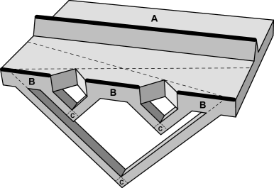
Figure 16: A clause gadget.

To connect together all the different gadgets we use structures called links. A link is a very thin prism with its two bases removed, and with a short link guard lying in the middle of an edge (see Figure 15). When we wish to connect two gadgets, we cut a hole in their surfaces, and we place a link stretching from one hole to the other. We will also make sure that no guard, other than its link guard, can see inside a link. Conversely, we will arrange the links in such a way that every link guard’s searchlight won’t interfere with the gadget guards. So, in every gadget there will be a thin illuminated polygon jutting from each of its links, which will be easily avoidable by the intruder. As a consequence, a link can be cleared by its guard only while both its bases are capped by some guards lying in the adjacent gadgets.

Given a boolean formula $\varphi$ in 3-conjunctive normal form, we construct a row of variable gadgets, one for every variable of $\varphi$, and a row of clause gadgets, one for every clause of $\varphi$. We arrange the variable gadgets so that all the A-sides are coplanar, and all the B-sides are coplanar. We arrange the clause gadgets similarly, and we place the two rows of gadgets in such a way that every distinguished side of every variable gadget can see every distinguished side of every clause gadget. We also associate the $i$-th B-side of a clause gadget to the $i$-th literal in the corresponding clause of $\varphi$, for $1\leqslant i\leqslant 3$.

Finally we add a bridge, which is constructed like a variable gadget, but it is not associated to any variable of $\varphi$. The bridge is shaped as a long, thin pole, whose guard lies over one of the long edges, and it is arranged in such a way that its distinguished sides can see the B-side of every clause gadget.

Connections

Then we connect the distinguished sides of our gadgets by placing links, as follows (refer to Figures 17 and 18).

• Connect the A-side of every clause gadget to both the A-side and the B-side of every variable gadget.

• Connect all the B-sides of every clause gadget to both the A-side and the B-side of the bridge.

• Connect all the C-sides of every clause gadget to both the A-side and the B-side of every variable gadget.

• Connect each B-side of each clause gadget to the A-side (resp. B-side) of the variable gadget corresponding to its associated literal, if that literal is negative (resp. positive) in $\varphi$.

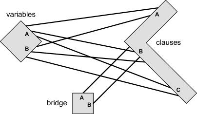
Figure 17: The relative positions of the gadgets and the bridge, with their links.

We can easily position the bridge so that it’s not accidentally hit by any link running between a variable gadget and a clause gadget, such as in Figure 17. We also want links to be pairwise disjoint. To achieve this, we consider any pair of intersecting links, and shrink them while translating them slightly, until their intersection vanishes. This can be accomplished without creating new intersections with other links, for example by making sure that the “new version” of each link is always strictly contained in its “previous version”.

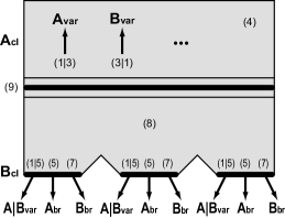
(a) clause gadget, top view

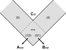
(b) clause gadget, C-side

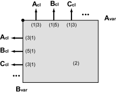
(c) variable gadget

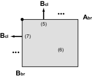
(d) bridge

Figure 18: The connections among gadgets, and their clearing order given in Theorem 10. The abbreviation “$\mathrm{A_{cl}}$” stands for “A-side of a clause gadget”, etc..

Reduction

Theorem 10.

3SSP is strongly NP-hard.

Proof.

Given an instance $\varphi$ of 3SAT, we construct the instance of 3SSP described above. It is indeed a polyhedron, because the bridge and all the variable gadgets are connected to all the clause gadgets. Moreover, the number of links is quadratic in the size of $\varphi$, and we may also assume that the coordinates of every vertex are rationals, with a number of digits that is polynomial in the size of $\varphi$. Removing the intersections between links takes polynomial time as well, hence the whole construction is computable in P.

Positive instances.

If $\varphi$ is satisfiable, we choose a satisfying assignment for its variables and give a search schedule that clears our polyhedron. Initially we aim each variable guard at its A-side (resp. B-side) if the corresponding variable is true (resp. false) in the chosen assignment. By assumption there is at least a true literal in every clause of $\varphi$. For each clause, we pick exactly one true literal, and aim the corresponding literal guard at the A-side of its clause gadget. We aim all the other literal guards at their respective B-sides. As a result, the A-side and the 3 C-sides of every clause gadget have the corresponding links capped by the literal guards. Finally, we aim the bridge guard at its A-side and put every separator in its leftmost position.

From this starting position, we specify a search schedule in 9 steps (refer to Figure 18).

1. Clear all the links that are capped by some variable guard. This is possible because, by construction, the other end of every such link is capped by some literal guard as well.

2. Clear every variable gadget by turning its guard. While this happens, the literal guards retain caps on their own side of the links cleared during Step 1, thus preventing recontamination.

3. Clear the remaining links connected to the A-side or to a C-side of a clause gadget. This is now possible because all the variable guards switched side in Step 2.

4. Aim at its B-side every literal guard that is currently aiming at its A-side. One half of each clause gadget gets cleared as a result, while the separator prevents the still uncapped links on the B-side from recontaminating the clear links on the A-side.

5. Clear the remaining links connected to a variable gadget, and clear the links capped by the bridge guard.

6. Clear the bridge by turning its guard to the B-side.

7. Clear the remaining links that connect the bridge with the clause gadgets.

8. Turn all the literal guards simultaneously, thus clearing the last half of each clause gadget, and capping the upper nooks. Since the three literal guards of a clause gadget are collinear, when they move together they act as a single exhaustive guard.

9. Clear every nook by turning the separators.

When this is done, the whole polyhedron is clear, which proves that the instance of 3SSP is searchable.

Negative instances.

Conversely, assuming that $\varphi$ is not satisfiable, we claim that the variable gadgets can never be all simultaneously clear, no matter what the guards do.

Recall that every A-side of every clause gadget is linked to both sides of every variable gadget. Hence, as soon as the A-side of any clause gadget is not covered by at least one literal guard, all the variable gadgets get immediately recontaminated, unless they were all clear in the first place. For the same reason, no variable gadget can ever be cleared while the A-side of some clause gadget is uncovered. Similarly, if a C-side of any clause gadget is not covered by at least one literal guard, all variable gadgets get recontaminated, and none of them can be cleared.

It follows that, in order for a schedule to start clearing any variable gadget, it must ensure that each clause gadget has exactly one literal guard covering the A-side and exactly two literal guards covering the C-sides. Moreover, the literal guards that cover the A-sides must be chosen once and for all. Indeed, whenever a schedule attempts to “switch gears” in some clause gadget and cover the A-side with a different literal guard, all the variable gadgets become immediately contaminated, and the search must start over.

Suppose that a schedule selects exactly one literal guard for each clause gadget, to cover its A-side. Since $\varphi$ is not satisfiable, there exist two selected literal guards $\ell_{1}$ and $\ell_{2}$ whose corresponding literals in $\varphi$ are a positive occurrence and a negative occurrence of the same variable $x$. Otherwise, if all selected literals were coherent, setting them to true would yield a satisfying assignment for the variables of $\varphi$, which is a contradiction.

But in this case, it turns out that the variable gadget corresponding to variable $x$ is impossible to clear. Indeed, there is a non-illuminated path connecting its A-side with its B-side, passing through the B-side of $\ell_{1}$, the bridge, and the B-side of $\ell_{2}$. Since $\ell_{1}$ and $\ell_{2}$ correspond to incoherent literals, their B-sides are connected to opposite sides of the same variable gadget, by construction.

Summarizing, all the variable gadgets are initially contaminated. In order to clear some of them, a schedule must first select a literal guard from each clause gadget and put it on its A-side. While that position is maintained, there is at least one variable gadget that is impossible to clear. As soon as one literal guard is moved, all the variable gadgets get recontaminated again. It follows that the variable gadgets can never be all clear at the same time, and in particular the polyhedron is unsearchable.

We gave a polynomial time reduction from 3SAT to 3SSP whose generated numerical coordinates are polynomially bounded in size, hence 3SSP is strongly NP-hard.∎

Optimization problems

Obviously, the previous theorem implies that the problems of minimizing search time and minimizing total angular movement are both NP-hard to approximate. The first problem stays NP-hard even when restricted to searchable instances, as proved in [9]. By further inspecting the construction given in that paper, it’s clear that the problem does not even have a PTAS, unless $\mbox{{P}}=\mbox{{NP}}$. Indeed, satisfiable boolean formulas are transformed into polyhedra searchable in $3$ seconds, while the unsatisfiable ones are transformed into polyhedra that are unsearchable in $3+\varepsilon$ seconds, for a suitable small-enough $\varepsilon>0$. On the other hand, similar results can be obtained also for the problem of minimizing total angular movement. There are several ways to rearrange the links in the construction employed in Theorem 10, so that the unsatisfiable boolean formulas are mapped into polyhedra that are indeed searchable, but only with very demanding schedules.

5.2 PSPACE-hardness of partial searchability

Here we introduce a slightly generalized problem: suppose the guards have to clear only a given subregion of the polyhedron, while the rest may remain contaminated. In particular, we stipulate that the target area that needs to be cleared is expressed as a ball, whose center and radius are given as input along with the polyhedron and the multiset of guards. We call the resulting problem 3-dimensional Partial Searchlight Scheduling Problem (3PSSP).

Definition 12 (3PSSP).

3PSSP is the problem of deciding if the guards of a given instance of 3SSP have a schedule that clears a ball with given center and radius.

The terminology defined in Section 2 for 3SSP extends straightforwardly to 3PSSP.

Next we are going to prove that 3PSSP is strongly PSPACE-hard, even restricted to orthogonal polyhedra. To do so, we give a reduction from the edge-to-edge problem for AND/OR constraint graphs in the nondeterministic constraint model described in [4].

Nondeterministic constraint logic machines

Consider an undirected 3-connected 3-regular planar graph, whose vertices can be of two types: AND vertices and OR vertices. Of the three edges incident to an AND vertex, one is called its output edge, and the other two are its input edges. Such a graph is (a special case of) a nondeterministic constraint logic machine (NCL machine). A legal configuration of an NCL machine is an orientation (direction) of its edges, such that:

• for each AND vertex, either its output edge is directed inward, or both its input edges are directed inward;

• for each OR vertex, at least one of its three incident edges is directed inward.

A legal move from a legal configuration to another configuration is the reversal of a single edge, in such a way that the above constraints remain satisfied (i.e., such that the resulting configuration is again legal).

Given an NCL machine with two distinguished edges $e_{a}$ and $e_{b}$, and a target orientation for each, we consider the problem of deciding if there are legal configurations $A$ and $B$ such that $e_{a}$ has its target orientation in $A$, $e_{b}$ has its target orientation in $B$, and there is a sequence of legal moves from $A$ to $B$. In a sequence of moves, the same edge may be reversed arbitrarily many times. We call this problem Edge-to-Edge for Nondeterministic Constraint Logic machines (EE-NCL).

A proof that EE-NCL is PSPACE-complete is given in [4], by a reduction from Quantified Boolean Formulas. Based on that reduction, we may further restrict the set of EE-NCL instances on which we will be working. Namely, we may assume that $e_{a}\neq e_{b}$, and that in no legal configuration both $e_{a}$ and $e_{b}$ have their target orientation.

Asynchrony

For our main reduction, it is more convenient to employ an asynchronous version of EE-NCL. Intuitively, instead of “instantaneously” reversing one edge at a time, we allow any edge to start reversing at any given time, and the reversal phase of an edge is not “atomic” and instantaneous, but may take any strictly positive amount of time. It is understood that several edges may be in a reversal phase simultaneously. While an edge is reversing, its orientation is undefined, hence it is not directed toward any vertex. During the whole process, at any time, both the above constraints on AND and OR vertices must be satisfied. We also stipulate that no edge is reversed infinitely many times in a bounded timespan, or else its orientation won’t be well-defined in the end. With these extended notions of configuration and move, and with the introduction of “continuous time”, EE-NCL is now called Edge-to-Edge for Asynchronous Nondeterministic Constraint Logic machines (EE-ANCL).

Despite its asynchrony, such new model of NCL machine has precisely the same power of its traditional synchronous counterpart.

Proposition 11.

$\textsc{EE-NCL}=\textsc{EE-ANCL}$.

Proof.

Obviously $\textsc{EE-NCL}\subseteq\textsc{EE-ANCL}$, because any sequence of moves in the synchronous model trivially translates into an equivalent sequence for the asynchronous model.

For the opposite inclusion, we show how to “serialize” a legal sequence of moves for an asynchronous NCL machine going from a legal configuration $A$ to configuration $B$ in a bounded timespan, in order to make it suitable for the synchronous model. An asynchronous sequence is represented by a set $S=\{(e_{m},s_{m},t_{m})\mid m\in M\}$, where $M$ is a set of “edge reversal events”, $e_{m}$ is an edge with a reversal phase starting at time $s_{m}$ and terminating at time $t_{m}>s_{m}$. For consistency, no two reversal phases of the same edge may overlap.

Because no edge can be reversed infinitely many times, $S$ must be finite. Hence we may assume that $M=\{1,\cdots,n\}$, and that the moves are sorted according to the (weakly increasing) values of $s_{m}$, i.e., $1\leqslant m<m^{\prime}\leqslant n\implies s_{m}\leqslant s_{m^{\prime}}$. Then we consider the serialized sequence $S^{\prime}=\{(e_{m},m,m)\mid m\in M\}$, and we claim that it is valid for the synchronous model, and that it is equivalent to $S$.

Indeed, each move of $S^{\prime}$ is instantaneous and atomic, no two edges reverse simultaneously, and every edge is reversed as many times as in $S$, hence the final configuration is again $B$ (provided that the starting configuration is $A$). We still have to show that every move in $S^{\prime}$ is legal. Let us do the first $m$ edge reversals in $S^{\prime}$, for some $m\in M$, starting from configuration $A$, and reaching configuration $C$. To prove that $C$ is also legal, consider the configuration $C^{\prime}$ reached in the asynchronous model at time $s_{m}$, according to $S$, right when $e_{m}$ starts its reversal phase (possibly simultaneously with other edges). By construction of $S^{\prime}$, every edge whose direction is defined in $C^{\prime}$ (i.e., every edge that is not in a reversal phase) has the same orientation as in $C$. It follows that, for each vertex, its inward edges in $C$ are a superset of its inward edges in $C^{\prime}$. By assumption on $S$, $C^{\prime}$ satisfies all the vertex constraints, then so does $C$, a fortiori. ∎

Corollary 12.

EE-ANCL is PSPACE-complete.

Proof.

Recall from [4] that EE-NCL is PSPACE-complete, and that $\textsc{EE-NCL}=\textsc{EE-ANCL}$ by Proposition 11. ∎

Building blocks

We realize a given NCL machine in terms of an orthogonal polyhedron consisting of three levels, called basement, floor and attic. The floor contains the actual AND/OR constraint graph, arranged as an orthogonal plane graph, and is completely unsearchable. The attic is reachable from the floor through two stairs, and contains the target ball that has to be cleared. The basement level is just a network of pipes connecting different parts of the floor to the stairs, whose purpose is to recontaminate the stairs and the attic unless the floor guards actually “simulate” the edges of an NCL machine.

It is well-known that any 3-regular planar graph can be embedded in the plane as an orthogonal drawing. For instance, we can employ the algorithm given in [7], which works with 3-connected 3-regular planar graphs, such as the constraint graphs of our NCL machines. The resulting drawing is orthogonal, in the sense that every edge is a sequence of horizontal and vertical line segments, which will be called subedges. For our construction, we turn every subedge into a thin-enough cuboid, then we place a subedge guard in the middle of each cuboid, on the bottom face, as depicted in Figure 19. The dotted squares between consecutive subedges are called trapdoors, and denote areas that will be attached to pipes and connected to other regions, as described later.

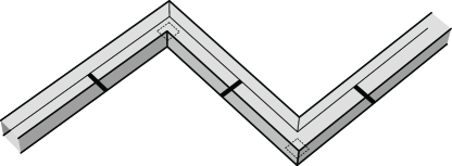
Figure 19: An edge, made of three orthogonal subedges.

Next we model OR vertices like in Figure 20. The three incoming cuboids carrying guards are subedges constructed in the previous paragraph. Again, the dotted square in the middle is a trapdoor that will be attached to pipes. Notice that the trapdoor completely belongs to the visibility region of each of the three guards, as the dotted lines suggest. Moreover, the two subedges coming from opposite directions are displaced, so they do not interfere with each other, in the sense that none of their two guards can see the opposite subedge through the end.

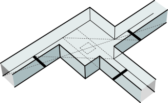
Figure 20: An OR vertex.

We model the AND vertices as shown in Figure 21. The output edge is the one whose guard sees both trapdoors, while the guards in the two input edges can see only one trapdoor each. We can always arrange the drawing of our graph by further bending its edges, in such a way that this construction is feasible (i.e., the output edge is located “between” the input edges), as suggested in Figure 22.

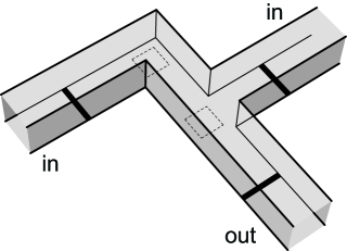
Figure 21: An AND vertex.

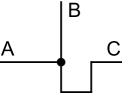
Figure 22: Rearranging the edges of an orthogonal drawing.

Recall that an instance of EE-ANCL comes with two distinguished edges $e_{a}$ and $e_{b}$, each of which is embedded in our construction as a sequence of cuboidal subedges. We select an internal subedge $s_{a}$ of $e_{a}$ (i.e., not the first, nor the last subedge of $e_{a}$) and an internal subedge $s_{b}$ of $e_{b}$, such that $s_{a}$ and $s_{b}$ run in two orthogonal directions. If no such subedges exist in our construction, we can further subdivide $e_{a}$ and $e_{b}$ into more small-enough “redundant” subedges, in order to obtain internal ones running in the desired directions. Recall also that both $e_{a}$ and $e_{b}$ come in EE-ANCL with a target orientation, which we want them to reach in order to solve the problem instance. Such target orientation is therefore naturally “inherited” by $s_{a}$ and $s_{b}$, too.

Let $\ell_{a}$ and $\ell_{b}$ be the two subedge guards lying in $s_{a}$ and $s_{b}$, respectively. We add two stairs going up to the attic, one for $\ell_{a}$ and one for $\ell_{b}$. Figure 23 shows a close-up of one end of $\ell_{a}$, where we have attached a stair (the two “incomplete” rectangles represent faces of $s_{a}$). Observe that, besides adding the polyhedral model of the stair to $s_{a}$, we also extend $\ell_{a}$ to the stair itself. The arrow attached to $\ell_{a}$ indicates the target orientation of $s_{a}$, inherited from the instance of EE-ANCL. There are two trapdoors, depicted as horizontal and vertical dotted squares. The horizontal trapdoor (marked as H in the picture) lies on the bottom face of an enclosed cuboidal region called alcove, whose opening is indicated by a darker vertical square. The alcove completely belongs to $\mathcal{V}(\ell_{a})$, and it can also be capped by the vertical guard showed in the picture, called stair guard. While the stair guard caps the alcove, it also covers the vertical trapdoor (marked as V). On the other hand, $\ell_{a}$ is able to cover the horizontal trapdoor. The top cuboid with dotted edges belongs to the attic, and is not considered part of the stair. The darker horizontal square that separates the attic from the stair is called attic entrance.

A similar construction is then repeated for $\ell_{b}$, and analogous remarks hold.

\psfrag{a}{$\ell_{a}$}\psfrag{b}{${}_{\alpha}$}\includegraphics[scale={1.75}]{figpspace8.eps}

Figure 23: A stair.

The whole attic is illustrated in Figure 24, where the darker squares denote the two attic entrances mentioned in the above paragraph, and the underlying cuboids with dotted edges belong to the stairs. A long L-shaped corridor, made of two orthogonal branches, connects the two entrances, and each entrance can be covered by an attic guard located at one end of the corridor. The small dot in the picture, in the middle of the corridor, denotes the target ball that has to be cleared by the guards. There is also a widening on one side of the corridor, which is not fully visible to the guards, and hence is a perpetual source of recontamination.

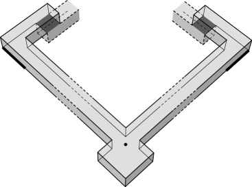
Figure 24: The attic.

To make sure that the floor is really unsearchable, we add a groove all around an end of each subedge guard, including $\ell_{a}$ and $\ell_{b}$, like in Figure 25. Every groove is always a source of recontamination, because some parts of it can never be seen by any guard, and cannot be isolated from the rest of the floor, either.

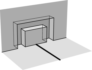
Figure 25: A close-up of a subedge guard, with its groove.

Finally, at the basement level, we add pipes, i.e., twisted chains of very thin cuboids, to connect pairs of trapdoors. We connect each trapdoor in each stair to every trapdoor in the floor (i.e., the trapdoors in the AND/OR vertices and the trapdoors between subedges). Since there are two different types of trapdoors in the stairs (horizontal and vertical), while the trapdoors in the floor are all horizontal, we need two types of pipes, as Figure 26 suggests. The end of a pipe that is marked as A goes into a stair trapdoor, whereas the end marked as B goes into a floor trapdoor. Observe that a pipe shaped like in Figure 26 can always connect a vertical stair trapdoor with any floor trapdoor, except when the latter lies exactly “behind” the former, and the lower part of the stair gets in the way. This can be easily prevented, for example by constructing a “thinner” version of the stair itself, such that no floor trapdoor lies completely behind the lower part of the stair (i.e., the part with the vertical trapdoor). In general, all pipes lie below the floor level, and their mutual intersections can be resolved by shrinking them, as already discussed in Subsection 5.1 for links.

\psfrag{a}{$\ell_{1}$}\psfrag{b}{$\ell_{2}$}\includegraphics[scale={0.9}]{figpspace2.eps}

\psfrag{a}{$\ell_{1}$}\psfrag{b}{$\ell_{2}$}\includegraphics[scale={0.9}]{figpspace9.eps}

Figure 26: Two pipes. The pipe in 26 connects two horizontal trapdoors, the pipe in 26 connects a vertical and a horizontal trapdoor.

Notice that two very small extra cuboids are attached to each pipe: these are called pits. Pits are unsearchable regions, but each pit can indeed be capped by a pipe guard. Such guards are also responsible for clearing the rest of the pipe, when both its ends A and B are capped by external searchplanes (belonging to a stair guard and to a subedge guard, respectively). Thus, by clearing a pipe we will mean clearing its chain of four bigger cuboids connecting A with B, disregarding the two pits.

Lemma 4.

While both its A and B ends are completely illuminated by external guards, a pipe can be cleared.

Proof.

A similar schedule works for both types of pipe. Referring to Figure 26, guard $\ell_{1}$ covers the darker square, allowing $\ell_{2}$ to clear two of the four cuboids. Then $\ell_{2}$ keeps capping its pit, while $\ell_{1}$ sweeps the remaining two cuboids, and caps the other pit. ∎

On the other hand, an uncapped pipe acts as a “one-way recontaminator” from B to A.

Lemma 5.

If neither A nor B is illuminated by external guards, then A is (partly) contaminated.

Proof.

If $\ell_{1}$ does not cap its pit, then it contaminates A. If $\ell_{1}$ caps its pit but $\ell_{2}$ does not, then the second pit contaminates A. If both guards cap both pits, then B contaminates A. ∎

Reduction

Theorem 13.

3PSSP is strongly PSPACE-hard, even restricted to orthogonal polyhedra.

Proof.

We give a reduction from EE-ANCL to 3PSSP, by proving that the target ball in the above construction is clearable if and only if the two distinguished edges $e_{a}$ and $e_{b}$ can be oriented in their target directions one after the other, by a legal sequence of asynchronous moves. Observe that our construction is obviously a polyhedron (it is indeed connected) whose vertices’ numerical coordinates may be chosen to be polynomially bounded in size, with respect to the size of the constraint graph. Moreover, the orthogonal drawing of the constraint graph can be obtained in linear time, as explained in [7].

Positive instances.

Suppose that the given instance of EE-ANCL is solvable. Then there exists a legal sequence $S$ of asynchronous moves that, starting from a configuration $A$ in which $e_{a}$ is in its target direction, ends in a configuration $B$ in which $e_{b}$ is in its target direction. By the assumptions we made on constraint graphs, $e_{a}\neq e_{b}$ and both $e_{a}$ and $e_{b}$ are reversed by $S$.

We start by “replicating” configuration $A$ on the subedge guards in our construction: if an edge has an orientation in $A$, then all its subedges in the drawing inherit its orientation, and all the corresponding subedge guards are oriented accordingly. As a result, every trapdoor in the floor (not the four trapdoors in the stairs) is covered by a guard, since $A$ is a legal configuration. Indeed, the structure of the AND/OR vertices that we built implies that the NCL constraints on a vertex are satisfied if and only if all the trapdoors in its polyhedral model are covered. Also the trapdoors between subedges happen to be covered, because all the guards in a subedge chain are oriented in the same “direction”. Incidentally, $\ell_{a}$ covers the horizontal trapdoor in its corresponding stair, as well. Next we cover the vertical trapdoors in both stairs with the stair guards, thus incidentally also capping both alcoves. Finally, we cover both attic entrances with the two attic guards.

In order to clear the target ball in the attic, our schedule proceeds as follows.

1. Clear the pipes that are attached to the stair trapdoors corresponding to $s_{a}$. This is feasible by Lemma 4, because both ends of such pipes are capped.

2. Replicate all the moves of $S$, with the correct timing. If a move reverses edge $\{u,v\}$ by turning it from vertex $u$ toward vertex $v$, we first reverse the guard corresponding to the subedge incident to $u$, then we reverse all the other subedge guards one by one in order, until we reverse the last guard in the chain, whose subedge is incident to $v$. By doing so, no trapdoor is ever uncovered, hence no pipe is recontaminated. Moreover, both $\ell_{a}$ and $\ell_{b}$ reverse during the process, incidentally clearing both alcoves, which are still capped by the stair guards.

3. Clear the pipes attached to the stair trapdoors corresponding to $s_{b}$, again by Lemma 4. Indeed, after Step 2, these pipes are all capped.

4. Clear the regions underlying the two attic entrances, by turning both stair guards by $\alpha$ (refer to Figure 23). Angle $\alpha$ is such that, in the end, both attic entrances are separated from the contaminated floor by the illuminated searchplanes of the stair guards. No contamination is possible through the stair trapdoors either, because all the pipes are still clear (their B ends are still capped).

5. Turn the two attic guards in concert, until they clear the target ball. No recontamination may occur through the attic entrances, whose underlying regions have effectively been cleared in Step 4, whereas the contaminated widening of the corridor is always separated from the portion of corridor that has been swept.

Negative instances.

Conversely, suppose that no legal sequence of asynchronous moves solves the given instance of EE-ANCL, and let us prove that the target ball in the attic is unclearable.

In order to clear the target ball, both attic guards have to turn in concert, away from the attic entrances. Indeed, just one guard is insufficient to clear anything. On the other hand, the attic guards cannot sweep toward the entrances, because of the unavoidable recontaminations from the widening in the corridor.

Therefore, while the attic guards operate, recontamination has to be avoided from the attic entrances. It follows that both stair guards must keep the attic separated from the unsearchable floor. Referring to Figure 23, each stair guard’s angle has to be at least $\alpha$.

When in that position, the stair guards cannot cover the vertical trapdoors, nor cap the alcoves. This means that all the pipes attached to a vertical trapdoor and both alcoves have to be simultaneously clear at some time $t$. According to Lemma 5, since the stair guards are not capping the A ends of those pipes, then their B ends have to be capped. In other words, all the trapdoors in the floor (not in the stairs) have to be covered. Equivalently, the subedge guards’ orientations must correspond to a legal configuration of an asynchronous NCL machine in the given constraint graph. If the orientations of the subedge guards in the chain corresponding to a same edge do not agree with each other, then that edge is considered in a reversal phase.

Recall that, in any legal configuration of the constraint graph, at least one of the two distinguished edges must be oriented opposite to its target direction (it cannot even be in a reversal phase), hence at least one horizontal trapdoor in a stair (say, the stair attached to $s_{a}$, without loss of generality) must be uncovered at time $t$. However, its alcove and attached pipes must indeed be clear, which means that $\ell_{a}$ has capped the pipes for some time, allowing them to clear themselves, and then has left the alcove for the last time at $t^{\prime}$, with $t^{\prime}<t$. Between time $t^{\prime}$ and time $t$, the orientation of the subedge guards must always correspond to a legal configuration of the constraint graph, otherwise the alcove just cleared by $\ell_{a}$ would be recontaminated by its pipes, again by Lemma 5.

Observe that, since at time $t^{\prime}$ guard $\ell_{a}$ is not oriented strictly opposite to its (inherited) target direction, then $\ell_{b}$ must be. But, at time $t$, also the alcove corresponding to $s_{b}$ must be clear, hence there must be some time $t^{\prime\prime}$, with $t^{\prime\prime}<t$, when $\ell_{b}$ last touched that alcove. Once again, between time $t^{\prime\prime}$ and time $t$, all the subedge guards must be oriented according to some legal configuration of the contraint graph.

Between time $t^{\prime}$ and time $t^{\prime\prime}$ (no matter which comes first), the search schedule must simulate an asynchronous legal sequence of moves between a configuration in which $e_{a}$ has its target orientation (more appropriately, $e_{a}$ is in a reversal phase), and one in which $e_{b}$ does. By hypothesis on the given constraint graph, such sequence of moves does not exist: notice in fact that a sequence of moves from $A$ to $B$ is legal if and only if its reverse sequence from $B$ to $A$ is legal.

This concludes the reduction. As a result, because EE-ANCL is PSPACE-complete by Corollary 12, 3PSSP is strongly PSPACE-hard. ∎

Observe that the above construction, regarded as an instance if 3SSP, is not viable, as in Definition 9. As a matter of fact, the presence of grooves around some guards, a widening in the attic’s corridor and pits in the pipes makes this polyhedron trivially unsearchable. Building a region that is never clear is certainly an effective way to force the recontamination of other critical regions when certain conditions are met. However, if we want our constructions to be viable instances of 3SSP, perhaps in order to prove its PSPACE-hardness, no such expedient is of any use, and cleverer tools have to be devised.

6 Concluding remarks

Summary

We modeled the 3-dimensional Searchlight Scheduling Problem as a searching problem in polyhedra, where guards are line segments emanating orientable half-planes of light. We showed that exhaustive guards act as the natural counterparts of boundary guards in the 2-dimensional version of the problem, in that the main positive results about SSP still hold for 3SSP restricted to instances with just exhaustive guards. By further exploiting the concept of exhaustive guard, we characterized the searchable instances of 3SSP with just one guard. Then we proved that $r^{2}$ guards are sufficient to search any polyhedron with $r>0$ notches, and that just $r$ guards lying over notches are sufficient to search an orthogonal polyhedron, thus partially settling Conjecture 1 in [9]. We also discussed some methods to speed up the search time by placing additional guards. Next we proved that deciding searchability of a polyhedron is strongly NP-hard, and briefly discussed the hardness of approximation of two related optimization problems. Finally, we showed that deciding if a given target area of an orthogonal polyhedron is searchable is strongly PSPACE-hard.

Further work

Several problems remain open. Settling Conjecture 1 in [9] would be the main priority. This has been accomplished for orthogonal polyhedra in Theorem 8, but for general polyhedra it turns out to be a surprisingly deep problem. One way to lower the quadratic bound on the number of guards would be to slightly modify the partition used in Theorem 6. Instead of aiming the guards at the angle bisectors of the notches, we could aim them in any direction, cut the polyhedron with the “extended” searchplanes, and still eliminate all the notches. The advantage would be that, by carefully choosing a plane for each notch that minimizes the intersections with other notches, the overall number of intersections could be significantly less than quadratic. Even if it is still quadratic in the worst case, it is likely much lower on average, with respect to any reasonable probability measure over polyhedra.

In the case of orthogonal polyhedra, the upper bound of $r$ guards given by Theorem 8 is also not known to be optimal. In fact, we believe that it can still be lowered by a constant factor.

The search time of the schedules given in Theorems 6 and 8 could be dramatically reduced by clearing several regions in parallel. For instance, in Theorem 8 we could turn in concert two guards whose fences do not bound a same cuboid. Generalizing, we could construct a graph $G$ on the set of notches, with an edge for every pair of notches whose fences bound a same cuboid. Then the search time would be proportional to the chromatic number $\chi(G)$, which is likely sublinear, at least on average.

The complexity of 3SSP could be considered also for a restricted set of instances, such as 0-genus polyhedra or orthogonal polyhedra. Moreover, the technique used for Theorem 10 could perhaps suggest a way to prove the NP-hardness of SSP. Adding new elements to SSP in order to increase its expressiveness, while preserving its 2-dimensional nature, could be an intermediate step. For example, we could introduce curtains, i.e., line segments that block visibility but don’t block movement. Then we could attempt to replicate the construction of Theorem 10 for this extension of SSP.

Similarly, we may try to modify the construction used in Theorem 13 to prove the PSPACE-hardness of 3SSP as well.

Acknowledgements

The author wishes to thank J. O’Rourke for his insightful comments.

This work was supported in part by MIUR of Italy under project AlgoDEEP prot. 2008TFBWL4.

References

[1]
B. Chazelle.
Convex partitions of polyhedra: a lower bound and worst-case optimal algorithm.
SIAM Journal on Computing, 13:488–507, 1984.
[2]
B. Chazelle and L. Palios.
Triangulating a nonconvex polytope.
Discrete and Computational Geometry, 5:505–526, 1990.
[3]
D. T. Lee and A. K. Lin.
Computational complexity of art gallery problems.
IEEE Transactions on Information Theory, 32:276–282, 1986.
[4]
R. A. Hearn and E. D. Demaine.
PSPACE-completeness of sliding-block puzzles and other problems through the nondeterministic constraint logic model of computation.
Theoretical Computer Science, 343:72–96, 2005.
Special issue “Game Theory Meets Theoretical Computer Science”.
[5]
K. J. Obermeyer, A. Ganguli, and F. Bullo.
A complete algorithm for searchlight scheduling.
International Journal of Computational Geometry & Applications, 21:101–130, 2011.
[6]
J. O’Rourke.
Art gallery theorems and algorithms.
Oxford University Press, 1987.
[7]
M. S. Rahman, S. Nakano, and T. Nishizeki.
A linear algorithm for optimal orthogonal drawings of triconnected cubic plane graphs.
In Proceedings of the Fifth Annual Symposium on Graph Drawing, pages 99–110, 1997.
[8]
K. Sugihara, I. Suzuki, and M. Yamashita.
The searchlight scheduling problem.
SIAM Journal on Computing, 19:1024–1040, 1990.
[9]
G. Viglietta and M. Monge.
The 3-dimensional searchlight scheduling problem.
In Proceedings of the 22nd Canadian Conference on Computational Geometry, pages 9–12, 2010.
[10]
M. Yamashita.
Private communication.
2010.
[11]
M. Yamashita, I. Suzuki, and T. Kameda.
Searching a polygonal region by a group of stationary -searchers.
Information Processing Letters, 92:1–8, 2004.