Photon echo quantum memories in inhomogeneously broadened two level atoms
Abstract
Here we propose a solid-state quantum memory that does not require spectral holeburning, instead using strong rephasing pulses like traditional photon echo techniques. The memory uses external broadening fields to reduce the optical depth and so switch off the collective atom-light interaction when desired. The proposed memory should allow operation with reasonable efficiency in a much broader range of material systems, for instance Er3+ doped crystals which have a transition at 1.5 . We present analytic theory supported by numerical calculations and initial experiments.
pacs:
3.67.Lx,82.53.Kp,78.90.+tI Introduction
Photon echo based techniques, particularly in rare earth ion dopants, have been long investigated for classical signal processing Mossberg (1982). More recently they have found use in quantum memory applications and are now leading the field with the longest storage times Fraval et al. (2005); Longdell et al. (2005), the highest efficiencies Hedges et al. (2010), broadest bandwidths Saglamyurek et al. (2010) and the highest time-bandwidth products Bonarota et al. (2010). The photon echo techniques used for quantum information applications differ from those used in the classical domain. Classical information processing using rare earth ion dopants relies on strong optical pulses to cause rephasing of the atomic coherences. Applying a similar approach in the quantum realm would be highly desirable, but analysis has shown that the basic techniques, namely the two-pulse Ledingham et al. (2010); Ruggiero et al. (2009) and three-pulse Sangouard et al. (2010) photon echo sequences, will not work as quantum memories.
This work proposes low noise photon echo techniques based on optical rephasing pulses that could be useful as quantum memories. We present analytical theory and initial experiments.
The two approaches currently used for photon echo quantum memories techniques, controlled reversible inhomogeneous broadening (CRIB)Moiseev and Kröll (2001); Kraus et al. (2006); Alexander et al. (2006); Longdell et al. (2008); Hétet et al. (2008); Hedges et al. (2010) and atomic frequency combs (AFC)de Riedmatten et al. (2008); Afzelius et al. (2009) both require spectral holeburning. This is the process where the inhomogeneously broadened absorption profile is modified by frequency selective optical pumping to shelving states.
For CRIB, spectral holeburning is used to create a spectrally narrow absorption feature. This is then broadened with a field gradient to accept the input light. The inverse spectral-width of the initial feature determines the storage time, and how far it is broadened determines the bandwidth. The light is then recalled by reversing the field gradient. To do this with high efficiency, significant optical thickness is required for the broadened feature, which means that extremely large optical thicknesses are required for the unbroadened feature. Hedges et al.Hedges et al. (2010) started with an absorption of -130 dB in the initial feature to achieve 69% efficiency with a time-bandwidth product only large enough to faithfully store one pulse.
In AFC protocols the material is prepared in a similar way to CRIB except that a number of narrow absorption features are created. Using this technique large bandwidth delays Bonarota et al. (2010) and reasonable efficiencies have also been demonstrated Sabooni et al. (2010).
With both CRIB and AFC methods, high efficiencies require efficient optical pumping and this requires long-lived shelving states. To date this has meant using shelving states in the dopant ions’ hyperfine structure. Our proposal does not rely on spectral holeburning, and the removal of this restriction is very appealing. The hyperfine splittings are generally less than 100 MHz, which makes large bandwidth operation for the AFC and CRIB protocols problematic. Saglamyurek et al. Saglamyurek et al. (2010) used a trick to overcome the problem of hyperfine structure and bandwidth with AFC memories. By choosing the correct comb spacing, they had the anti-holes that result from spectral holeburning appearing on top of the comb teeth. The downside of this approach is that high finesse frequency combs are not possible, severely limiting the efficiency.
Another reason to avoid spectral holeburning is the requirement of efficient holeburning limits the choice of material systems. For example, while single photon memories have been demonstrated at telecommunication wavelengths using erbium Lauritzen et al. (2010), the lack of an efficient holeburning mechanism severely limited the memory efficiency.
Ensemble quantum memories rely on the fact that the collective interaction with an optical field is greatly enhanced for systems with reasonable optical depths. The problem with optically rephased memories is that the strong optical rephasing pulses necessarily invert the population, this causes gain and the associated noise.
Here we propose avoiding this problem by using a perturbing field to spectrally broaden the ensemble while in the excited state to the point where it is optically thin. This removes the collective enhancement and stops the unwanted noise processes. We call this method where both reversible inhomogeneous broadening and optical rephasing methods are used hybrid photon echo rephasing (HYPER).
Another approach that avoids the use of spectral holeburning by using Raman echoes has also been proposed Moiseev (2011).
II Description
The hybrid photon echo rephasing technique uses a combination of broadening field pulses and optical pulses to rephase a small optical input pulse. For what follows we shall assume that the broadening field is an electric field gradient which causes inhomogeneous broadening due to the atom’s linear Stark effect. Using a linear electric field gradient is not a fundamental requirement of the HYPER protocol. As long as the broadening is completely reversed any applied field will be acceptable. The case of a linear field gradient is considered here as this is what was used in the experimental work.
Using two -pulses allows the ions to rephase near the ground state, forming an echo of the normal two pulse echo (2PE). This is beneficial as an echo forming in the excited state is inherently noisy. The electric field gradients are applied at appropriate times to eliminate excited state noise on the output.
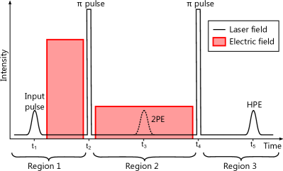
The pulse sequence, shown in Fig. 1, has three time regions. In the first region () one or more input pulses are applied followed by the application of a broadening field. A pulse is applied at . The -pulse creates gain which a 2PE would ordinarily propagate through and thus undergo amplification. The effect of broadening the ensemble is to reduce the gain, and the two pulse echo, to an arbitrarily low level. In doing so the troublesome collective interaction between the light and the atoms is effectively turned off while the atoms are in the excited state.
While the dephasing caused by the applied broadening stops the two pulse echo forming, so long as the broadening applied before and after the first -pulse are balanced an echo of the 2PE will form after a second -pulse. This is the output from the memory. We call this type of echo, which involves both static and controlled inhomogeneous broadening a hybrid photon echo (HPE).
III Analytical Theory
Here we use the same theoretical description that was developed for rephased amplified spontaneous emission Ledingham et al. (2010). It is assumed that the input light to all regions is weak compared to a -pulse and that the rephasing pulses are ideal -pulses.
Figure 1 shows the pulse sequence with three different time regions. The equations of motion for time region 1 before the Stark shift is applied are as follows,
| (1a) | ||||
| (1b) | ||||
Here, is the quantum optical (atomic) field operator, subscript 1 indicates region 1, is the optical depth parameter and represents the detuning of the atom. The solution for the atomic field (Eq. 1a) is given by
| (2) |
To obtain the solution for the optical field we Fourier transform Eq. 2 with respect to time and substitute into the transformed version of Eq. 1b. The solution in the time domain is found to be
| (3) |
where is defined as . We now have the complete solution in region 1 for before the Stark shifting fields are applied.
We now assume that the Stark shifting field is turned on just before the first -pulse and is strong and temporally short, allowing the dynamics of the optical field to be ignored. The Stark shifting field alters an atom’s detuning dependent on its position by such that , whereas the -pulse inverts the atoms leading to . The Stark shift and -pulse result in the following transformation on the atomic field at the region 2 () boundary,
| (4) |
where . Here, is the intensity of the Stark shifting field and is the duration of that field.
Under the small input pulse approximation the atoms in region 2 are all near the excited state.
A temporally long Stark shifting pulse is applied during all of region 2. The equations of motion are given by
| (5a) | ||||
| (5b) | ||||
where again the subscript denotes region. It is noted that these equations are similar in form to the region 1 equations, with the atomic fields daggered due to the -pulse and the detuning is shifted with a field intensity such that . Also, a sign change in front of the optical field in the atomic equation of motion is present.
The atomic field solution for region 2 is given by
| (6) |
Using the region 2 boundary condition stated earlier, the optical field solution for region 2 is found in a similar fashion as for region 1:
| (7) |
where we have defined the following operators
This completes the solution for region 2. It is noted that when the Stark fields are set to zero, the two pulse photon echo solutions are retained with efficiency as expected.
We can now form the region 3 boundary condition, in a similar fashion to the region 2 boundary condition, namely .
The equations of motion that describe the dynamics of region 3 are exactly those stated for region 1, Eqs. 1a and 1b. Hence the optical solution for region 3 is identical in form to Eq. 3, with subscript and . For balanced Stark fields, the output optical solution in region 3 is
| (8) |
where we have defined the operator
In the limit of large Stark shift, Eq. III becomes
| (9) |
The solution has three terms. The first term is the inevitable optical vacuum input at the region 3 time boundary which decays as a function of the optical depth. The second term is the HYPER echo which forms at a time with . This echo has a maximum efficiency of at . The third term contains the atomic degrees of freedom. If counter-propagating -pulses are used, causing the echo to be emitted in the backward direction, 100% efficiency is possible (see appendix).
It can be seen that the Stark shifting field over region 2 eliminates contributions from region 2 on the region 3 output. Taking the limit of infinite Stark shift is physically equivalent to decoupling the optical and atomic fields in the equations of motion in region 2, thus ‘switching off’ the collective atom-light interaction in this region and reducing the noise on the output field. In the decoupled regime, the atomic boundary condition at region 3 is found by propagating the region 2 boundary condition forward in time by . The result obtained for the output field in region 3 is identical to Eq. III.
IV Echo demonstration
The experimental setup used is shown in Fig. 2, a modified Coherent 699 dye laser with sub 5 kHz linewidth drives the 3H4 1D2 transition, at 605.977 nm, in a Pr3+:Y2SiO5 crystal. The sample is oriented such that the laser propagates along the crystal b-axis, and is linearly polarized along the D2-axis.
The crystal is surrounded by four electrodes in a quadrupole arrangement that enabled an electric field gradient to be produced along the direction of propagation. The electric fields used in region 1 varied from V/cm over the optical path length, and were directed parallel to the b-axis. Using the tabled value of the Stark shiftGraf et al. (1998), this results in detunings of approximately MHz. The direction of the applied electric field was parallel to the crystals b-axis. The entire sample/electrode setup is mounted inside a cryostat and cooled to . Two acousto-optic modulators (AOMs) were used to gate the laser beam to produce the input pulses. The AOMs also introduce a net 10 MHz frequency shift, enabling the light exiting the crystal to be detected with phase sensitive heterodyne detection.
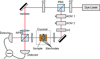
Figure 3 shows the intensity of the light exiting the sample during a hybrid photon echo sequence. Three optical pulses are applied, the input pulse and two -pulses. The input pulse is a Gaussian with a full width at half maximum (FWHM) power of , and the transmitted portion appears at (i). In the absence of the Stark field, the first -pulse (ii) causes a 2PE (iii). The 2PE is rephased to form the hybrid photon echo at (vi). The two -pulses were not placed symmetrically about the 2PE so that the three pulse photon echo (3PE) at (v), due to the input and two -pulses, is separated in time from the HPE.
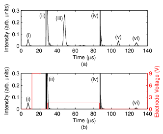
The amplitude of the pulses were calibrated by applying a 2PE sequence with the first pulse half the length of the second. The lengths that maximised the size of the echo were taken as being a pulse and pulse.
Applying the electric field to the sample causes the intensity of the 2PE to be reduced by through the mechanism explained earlier. The 3PE also experiences a large reduction in intensity, which can be explained using similar reasoning. The HPE is still formed albeit with reduced efficiency. We believe this reduction in efficiency is most likely due to imperfect balancing of the broadening applied before and after the first -pulse.
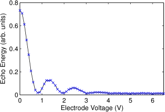
Figure 4 shows the intensity of the 2PE as the size of the broadening field is increased. The electric field varies linearly along the propagation axis, resulting in a top-hat distribution of frequency shifts. Thus the phase shifts of the ions will have a top-hat distribution as the 2PE forms. This leads to a sinc-squared behaviour in the energy of the 2PE, analogous to a single slit diffraction pattern.
Due to optical pumping distributing population amongst the hyperfine levels Pr3+:Y2SiO5 exhibits spectral holeburning Holliday et al. (1993). Optical repumping was used so that the number of ions and thus the optical depth remained consistent between shots. The laser was first scanned over the spectral region of interest to burn a wide spectral hole. This hole was then filled using laser light pulses detuned by a specific combination of the hyperfine splittings. Varying the number of these repumping pulses allowed for variation of the optical depth.
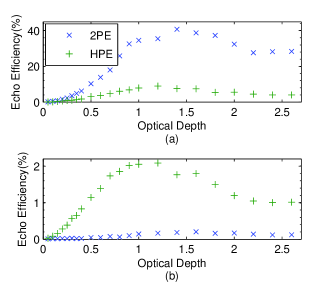
The efficiency of the 2PE and HPE was measured over a range of optical depths (see Fig. 5). The maximum efficiency for the 2PE occurs at an optical depth of around 1.5, while the maximum efficiency of the HPE is at an optical depth of around 1.2. This is independent of whether the electric field was on or off. The maximum 2PE efficiency reduces from 40% to less than 0.3% when 9 V was applied to the electrodes.
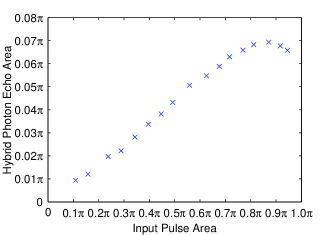
In order to verify the linearity and determine the efficiency of the HPE, the area of the input pulse was compared to the area of the output pulse (see Fig. 6). The length of the input pulse was set to (FWHM), whilst the amplitude of the pulse was altered by adjusting the radio frequency power applied to AOM2. The optical depth for this experiment was set to 1. As shown in Fig. 6, the relationship between input pulse and output pulse is linear for input pulses small compared to a -pulse and then flattens off for more intense pulses.
V Noise Measurements
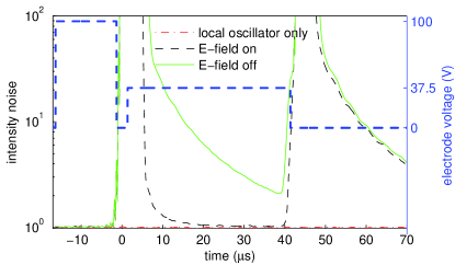
To characterize the noise properties, the heterodyne signal of the HYPER pulse sequence was recorded with no input pulse, both with and without the electric field applied. The Pr3+:Y2SiO5 sample used for the noise measurements was 4x4x20 mm (20 mm along the beam propagation direction), doped at 0.005%. Before the initial -pulse, 100 V is applied to the two electrodes. In this alternate sample geometry this results in an electric field varying from -30 V/cm to +30 V/cm along the 20 mm axis, corresponding to a frequency shift of approximately MHz. This voltage is decreased to 37.5 V for the longer period between the -pulses to maintain a zero net Stark shift such that an input pulse would be rephased as a HPE.
The noise was calculated as follows. For each of 30 000 shots, the time-domain signal was multiplied by the temporal envelope of the would-be 2PE (FWHM of 1.8 s, centered 15 s after the first -pulse), numerically heterodyned (optical beat frequency here was 6 MHz) down to DC and summed. This quantifies the field amplitude in the 2PE mode for each shot. Taking the variance across all shots yields a value related to the average field intensity in this specific mode. For normalization purposes, the shot-noise (noise level with local oscillator on, but signal beam blocked) was measured as the variance in an equivalent mode, but with the temporal envelope shifted to before the first -pulse.
At an optical depth of 0.15, the quadrature variances in the echo mode without the electric field applied were measured as 8.648% normalized to the shot-noise level. With the electric field applied, the noise reduces approximately two orders of magnitude to 1.0454%, a level indistinguishable from the vacuum. Figure 7 shows the averaged time dependence of the noise in the spectral mode of the echo. The experiment was repeated for larger optical depths of 0.36 and 0.98, where the noise was similarly reduced by factors of 150 and 160 respectively.
There are three mechanisms through which the applied field gradient decreases the noise. Firstly, the gain feature created by the initial -pulse is broadened in frequency, and therefore the number of excited ions generating amplified spontaneous emission in the original frequency window is reduced. Secondly, there are ground-state ions Stark-shifted into the detection frequency window which increases the absorption. Assuming a perfect -pulse with a 1 MHz width, and an optical depth of 1, the expected reduction of noise due to these two effects is only 5. However, in practice the -pulse is far from perfect and most of the ions in the ensemble see a pulse area greater or less than (due largely to the Gaussian spatial profile of the pulse intensity). This and structure on the inhomogeneous line results in a large free induction decay (FID). The third and most significant effect of the applied electric field is the reduction of this FID.
VI Discussion and Classical Simulation
There are two areas where these initial experiments need to be improved before the proposed memory can fulfil its theoretical promises. The demonstrated memory is of low efficiency and noisy. The noise measurements, Fig. 7, show that the broadening field is successful in decoupling excited atoms from the output field while they are inverted, but there is excess noise in the time region where the light would be recalled from the memory.
The predominant reason for this noise is the imperfect -pulses resulting in random FIDs due to structure in the inhomogeneous line. In systems that have long lived spectral holes like Pr3+:Y2SiO5 this structure is hard to avoid. A four-level echo protocol provides a way around this problem Beavan et al. (2011). Experiments involving Tm3+:YAG, which has short lived holes, have achieved -pulses without measurable random FIDs led .
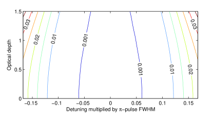
Even in the absence of structure on the inhomogeneous line, this HYPER quantum memory scheme is still reliant on doing -pulses well, but less sensitively. In the output region the solution for the time domain is an expression like Eq. 3, but with the subscript 1 replaced by 3, for region 3. Here represents the light incident on the crystal during the recall of the light (usually the vacuum). The term that includes represents that light emitted from the sample due to any excitation in the crystal after the second -pulse. In the case of perfect -pulses and vacuum input, will represent ground state atoms. In the case of imperfect -pulses the atoms will have some unwanted excitation resulting in noise. The ability to apply accurate -pulses has already received careful study Zafarullah et al. (2007); Ruggiero et al. (2010). Semi-classical 1-D numerical calculations, presented in Fig. 8, show that in the case of no transverse variation in the optical intensity, atomic population very close to the ground can be achieved over a significant fraction of the bandwidth of the pulses. This in turn means that the amount of noise in the output would be reduced to much lower than one photon per spatio-temporal mode. The fact that there will be spontaneous emission while the atoms are excited will be another noise process, but like the effect of imperfect -pulses this noise would not be phase matched with the echo. As long as the population is predominantly in the ground state when the echo is retrieved, the amount of noise will be much less than one photon per spatio-temporal mode.
VII Conclusion
We propose and present initial experiments for a new quantum memory protocol. The proposal uses strong rephasing pulses rather than structure in the inhomogeneous line made with spectral holeburning. Noise associated with echoes forming in the excited state is avoided by using electric field gradients to generate artificial inhomogeneous broadening while the media is in the excited state. We present a demonstration of these echoes as well as initial noise measurements. In these experiments the echoes were noisy due to random FIDs arising from structure on the inhomogeneous line rather than amplified spontaneous emission from the excited state atoms. In order to make the memory quiet these random FIDs must be avoided. Furthermore to ensure the atoms form the echo while close to the ground state accurate -pulses will be required. Both of these steps should be technically feasible.
Note added: Recently, a new proposal has been developed that uses some of these ideas rose . This new proposal is attractive in that it removes the need for auxiliary broadening fields.
VIII Acknowledgments
We thank the referee who suggested we look at backward retrieval which led to the material in the appendix.
DLM, PML, WRN and JJL were supported by the New Zealand Foundation for Research Science and Technology under Contract No. NERF-UOOX0703.
SEB, MPH, and MJS were supported by the Australian Research Council Centre of Excellence for Quantum Computation and Communication Technology (Project No. CE11E0096).
*
Appendix A Backward Retrieval
Here we show that similar to other proposals Moiseev and Kröll (2001); Afzelius et al. (2009); rose , in the limit of large optical depth the memory has perfect efficiency when the echo is retrieved from the sample in the backward direction.
Here we consider a sample that lies from to . Equations 1a and 1b are equations of motion for the atomic () and optical () modes propagating in the forward direction, toward larger values of . For clarity the labels and will be used for these quantities. The equations of motion for the counter-propagating, ‘backward’ fields are the same as the forward case except for a minus sign in Eq. 1b
| (10) |
The treatment in this appendix is semi-classical. This simplifies the expressions greatly because the amplitudes of modes with no excitation can be set to zero, and then ignored. A quantum treatment will yield the same results, but with the appropriate addition of vacuum modes to preserve the commutation relations in the presence of loss.
We consider an input field that is zero for , and atomic modes that are initially in the ground state. In this case, we can see from Eqs. 2 and 3 that the forward propagating atomic modes at are given by
| (11) | |||||
Here is the Fourier transform of . The upper limit on the integral can be changed to infinity because the input field is zero for .
We reduce the dynamics during the rephasing period, the time period between when the broadening field is first turned on and the second rephasing pulse, to an instantaneous operation at . For the case of counter-propagating -pulses this has the effect
| (12) |
The time delay, , is the difference between how long the atoms are in the excited state and the ground state, during the rephasing period. Analogous to Eq. 3 we have for
| (13) |
The first term on the right-hand side can be ignored because no light is incident on the end of the crystal during the retrieval process. The integral can easily be computed, resulting in a value for of
| (14) |
or alternatively
| (15) |
leading to an efficiency that varies with optical depth as . This is equal to 1 for large .
References
- Mossberg (1982) T. W. Mossberg, Opt. Lett. 7, 77 (1982).
- Fraval et al. (2005) E. Fraval, M. J. Sellars, and J. J. Longdell, Phys. Rev. Lett. 95, 030506 (2005).
- Longdell et al. (2005) J. J. Longdell, E. Fraval, M. J. Sellars, and N. B. Manson, Phys. Rev. Lett. 95, 063601 (2005).
- Hedges et al. (2010) M. P. Hedges, J. J. Longdell, Y. Li, and M. J. Sellars, Nature (London) 465, 1052 (2010).
- Saglamyurek et al. (2010) E. Saglamyurek, N. Sinclair, J. Jin, J. A. Slater, D. Oblak, F. Bussiéres, M. George, R. Ricken, W. Sohler, and W. Tittel, Nature (London) 469, 512 (2010).
- Bonarota et al. (2010) M. Bonarota, J.-L. Le Gouët, T. Chaneliére, New J. Phys. 13, 013013 (2011).
- Ledingham et al. (2010) P. M. Ledingham, W. R. Naylor, J. J. Longdell, S. E. Beavan, and M. J. Sellars, Phys. Rev. A 81, 012301 (2010).
- Ruggiero et al. (2009) J. Ruggiero, J.-L. Le Gouët, C. Simon, and T. Chanelière, Phys. Rev. A 79, 053851 (2009).
- Sangouard et al. (2010) N. Sangouard, C. Simon, J. Minár, M. Afzelius, T. Chanelière, N. Gisin, J.-L. Le-Gouët, H. de Riedmatten, and W. Tittel, Phys. Rev. A 81, 062333 (2010).
- Moiseev and Kröll (2001) S. A. Moiseev and S. Kröll, Phys. Rev. Lett. 87, 173601 (2001).
- Kraus et al. (2006) B. Kraus, W. Tittel, N. Gisin, M. Nilsson, S. Kröll, and J. I. Cirac, Phys. Rev. A 73, 020302(R) (2006).
- Alexander et al. (2006) A. L. Alexander, J. J. Longdell, M. J. Sellars, and N. B. Manson, Phys. Rev. Lett. 96, 043602 (2006).
- Longdell et al. (2008) J. J. Longdell, G. Hétet, P. K. Lam, and M. J. Sellars, Phys. Rev. A 78, 032337 (2008).
- Hétet et al. (2008) G. Hétet, J. J. Longdell, A. L. Alexander, P. K. Lam, and M. J. Sellars, Phys. Rev. Lett. 100, 023601 (2008).
- de Riedmatten et al. (2008) H. de Riedmatten, M. Afzelius, M. U. Staudt, C. Simon, and N. Gisin, Nature (London) 456, 773 (2008).
- Afzelius et al. (2009) M. Afzelius, C. Simon, H. de Riedmatten, and N. Gisin, Phys. Rev. A 79, 052329 (2009).
- Sabooni et al. (2010) M. Sabooni, F. Beaudoin, A. Walther, N. Lin, A. Amari, M. Huang, S. Kröll, Phys. Rev. Lett. 105, 060501 (2010).
- Lauritzen et al. (2010) B. Lauritzen, J. Minár, H. de Riedmatten, M. Afzelius, N. Sangouard, C. Simon, and N. Gisin, Phys. Rev. Lett. 104, 080502 (2010).
- Moiseev (2011) S. A. Moiseev, Phys. Rev. A 83, 12307 (2011).
- Graf et al. (1998) F. R. Graf, A. Renn, G. Zumofen, and U. P. Wild, Phys. Rev. B 58, 5462 (1998).
- Holliday et al. (1993) K. Holliday, M. Croci, E. Vauthey, and U. P. Wild, Phys. Rev. B 47, 14741 (1993).
- Beavan et al. (2011) S. E. Beavan, P. M. Ledingham, J. J. Longdell, and M. J. Sellars, Opt. Lett. 36, 1272 (2011).
- (23) P. M. Ledingham et al. (unpublished).
- Zafarullah et al. (2007) I. Zafarullah, M. Tian, T. Chang, and W. R. Babbitt, J. Lumin. 127, 158 (2007).
- Ruggiero et al. (2010) J. Ruggiero, T. Chanelière, and J.-L. Le Gouët, J. Opt. Soc. Am. B 27, 32 (2010).
- (26) V. Damon, M. Bonarota, A. Louchet-Chauvet, T. Chanelière, and J.-L. Le Gouët, ArXiv quant-ph/1104.4875.