030001 2011 G. C. Barker B. Blasius, ICBM, University of Oldenburg, Germany. 030001

We study the propagation of an SIR (susceptible–infectious–recovered) disease over an agent population which, at any instant, is fully divided into couples of agents. Couples are occasionally allowed to exchange their members. This process of couple recombination can compensate the instantaneous disconnection of the interaction pattern and thus allow for the propagation of the infection. We study the incidence of the disease as a function of its infectivity and of the recombination rate of couples, thus characterizing the interplay between the epidemic dynamics and the evolution of the population’s interaction pattern.

SIR epidemics in monogamous populations with recombination

99 inst1 Consejo Nacional de Investigaciones Científicas y Técnicas, Centro Atómico Bariloche e Instituto Balseiro, 8400 Bariloche, Río Negro, Argentina.

1 Introduction

Models of disease propagation are widely used to provide a stylized picture of the basic mechanisms at work during epidemic outbreaks and infection spreading [1]. Within interdisciplinary physics, they have the additional interest of being closely related to the mathematical representation of such diverse phenomena as fire propagation, signal transmission in neuronal axons, and oscillatory chemical reactions [2]. Because this kind of model describes the joint dynamics of large populations of interacting active elements or agents, its most interesting outcome is the emergence of self-organization. The appearance of endemic states, with a stable finite portion of the population actively transmitting an infection, is a typical form of self-organization in epidemiological models [3].

Occurrence of self-organized collective behavior has, however, the sine qua non condition that information about the individual state of agents must be exchanged between each other. In turn, this requires the interaction pattern between agents not to be disconnected. Fulfilment of such requirement is usually assumed to be granted. However, it is not difficult to think of simple scenarios where it is not guaranteed. In the specific context of epidemics, for instance, a sexually transmitted infection never propagates in a population where sexual partnership is confined within stable couples or small groups [4].

In this paper, we consider an SIR (susceptible–infectious–recovered) epidemiological model [3] in a monogamous population where, at any instant, each agent has exactly one partner or neighbor [4, 5]. The population is thus divided into couples, and is therefore highly disconnected. However, couples can occasionally break up and their members can then be exchanged with those of other broken couples. As was recently demonstrated for SIS models [6, 7], this process of couple recombination can compensate to a certain extent the instantaneous lack of connectivity of the population’s interaction pattern, and possibly allow for the propagation of the otherwise confined disease. Our main aim here is to characterize this interplay between recombination and propagation for SIR epidemics.

In the next section, we review the SIR model and its mean field dynamics. Analytical results are then provided for recombining monogamous populations in the limits of zero and infinitely large recombination rate, while the case of intermediate rates is studied numerically. Attention is focused on the disease incidence –namely, the portion of the population that has been infectious sometime during the epidemic process– and its dependence on the disease infectivity and the recombination rates, as well as on the initial number of infectious agents. Our results are inscribed in the broader context of epidemics propagation on populations with evolving interaction patterns [4, 5, 8, 9, 10, 11].

2 SIR dynamics and mean field description

In the SIR model, a disease propagates over a population each of whose members can be, at any given time, in one of three epidemiological states: susceptible (S), infectious (I), or recovered (R). Susceptible agents become infectious by contagion from infectious neighbors, with probability $\lambda$ per neighbor per time unit. Infectious agents, in turn, become recovered spontaneously, with probability $\gamma$ per time unit. The disease process S $\to$ I $\to$ R ends there, since recovered agents cannot be infected again [3].

With a given initial fraction of S and I–agents, the disease first propagates by contagion but later declines due to recovery. The population ends in an absorbing state where the infection has disappeared, and each agent is either recovered or still susceptible. In this respect, SIR epidemics differs from the SIS and SIRS models, where –due to the cyclic nature of the disease,– the infection can asymptotically reach an endemic state, with a constant fraction of infectious agents permanently present in the population.

Another distinctive equilibrium property of SIR epidemics is that the final state depends on the initial condition. In other words, the SIR model possesses infinitely many equilibria parameterized by the initial states.

In a mean field description, it is assumed that each agent is exposed to the average epidemiological state of the whole population. Calling $x$ and $y$ the respective fractions of S and I–agents, the mean field evolution of the disease is governed by the equations

$$\begin{array}[]{lll}\dot{x}&=&-k\lambda xy,\\ \dot{y}&=&k\lambda xy-y,\end{array}$$ (1)

where $k$ is the average number of neighbors per agent. Since the population is assumed to remain constant in size, the fraction of R–agents is $z=1-x-y$. In the second equation of Eqs. (1), we have assigned the recovery frequency the value $\gamma=1$, thus fixing the time unit equal to $\gamma^{-1}$, the average duration of the infectious state. The contagion frequency $\lambda$ is accordingly normalized: $\lambda/\gamma\to\lambda$. This choice for $\gamma$ will be maintained throughout the remaining of the paper.

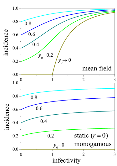
Figure 1: SIR epidemics incidence (measured by the final fraction of recovered agents $z^{*}$) as a function of the infectivity (measured by the product of the mean number of neighbors times the infection probability per time unit per infected neighbor, $k\lambda$), for different initial fractions of infectious agents, $y_{0}$. Upper panel: For the mean field equations (1). Lower panel: For a static (non-recombining) monogamous population, described by Eqs. (3) with $r=0$.

The solution to Eqs. (1) implies that, from an initial condition without R–agents, the final fraction of S–agents, $x^{*}$, is related to the initial fraction of I–agents, $y_{0}$, as [1]

$$x^{*}=1-(k\lambda)^{-1}\log[(1-y_{0})/x^{*}].$$ (2)

Note that the final fraction of R–agents, $z^{*}=1-x^{*}$, gives the total fraction of agents who have been infectious sometime during the epidemic process. Thus, $z^{*}$ directly measures the total incidence of the disease.

The incidence $z^{*}$ as a function of the infectivity $k\lambda$, obtained from Eq. (2) through the standard Newton–Raphson method for several values $y_{0}$ of the initial fraction of I–agents, is shown in the upper panel of Fig. 1. As expected, the disease incidence grows both with the infectivity and with $y_{0}$. Note that, on the one hand, this growth is smooth for finite positive $y_{0}$. On the other hand, for $y_{0}\to 0$ (but $y_{0}\neq 0$) there is a transcritical bifurcation at $k\lambda=1$. For lower infectivities, the disease is not able to propagate and, consequently, its incidence is identically equal to zero. For larger infectivities, even when the initial fraction of I–agents is vanishingly small, the disease propagates and the incidence turns out to be positive. Finally, for $y_{0}=0$ no agents are initially infectious, no infection spreads, and the incidence thus vanishes all over parameter space.

3 Monogamous populations with couple recombination

Suppose now that, at any given time, each agent in the population has exactly just one neighbor or, in other words, that the whole population is always divided into couples. In reference to sexually transmitted diseases, this pattern of contacts between agents defines a monogamous population [5]. If each couple is everlasting, so that neighbors do not change with time, the disease incidence should be heavily limited by the impossibility of propagating too far from the initially infectious agents. At most, some of the initially susceptible agents with infectious neighbors will become themselves infectious, but spontaneous recovery will soon prevail and the disease will disappear.

If, on the other hand, the population remains monogamous but neighbors are occasionally allowed to change, any I–agent may transmit the disease several times before recovering. If such changes are frequent enough, the disease could perhaps reach an incidence similar to that predicted by the mean field description, Eq. (1) (for $k=1$, i.e. with an average of one neighbor per agent).

We model neighbor changes by a process of couple recombination where, at each event, two couples $(i,j)$ and $(m,n)$ are chosen at random and their partners are exchanged [6, 7]. The two possible outcomes of recombination, either $(i,m)$ and $(j,n)$ or $(i,n)$ and $(j,m)$, occur with equal probability. To quantify recombination, we define $r$ as the probability per unit time that any given couple becomes involved in such an event.

A suitable description of SIR epidemics in monogamous populations with recombination is achieved in terms of the fractions of couples of different kinds, $m_{\rm SS}$, $m_{\rm SI}$, $m_{\rm II}$, $m_{\rm IR}$, $m_{\rm RR}$, and $m_{\rm SR}=1-m_{\rm SI}-m_{\rm II}-m_{\rm IR}-m_{\rm RR}$. Evolution equations for these fractions are obtained by considering the possible transitions between kinds of couples due to recombination and epidemic events [7]. For instance, partner exchange between two couples (S,S) and (I,R) which gives rise to (S,I) and (S,R), contributes positive terms to the time derivative of $m_{\rm SI}$ and $m_{\rm SR}$, and negative terms to those of $m_{\rm SS}$ and $m_{\rm IR}$, all of them proportional to the product $m_{\rm SS}m_{\rm IR}$. Meanwhile, for example, contagion can transform an (S,I)–couple into an (I,I)–couple, with negative and positive contributions to the variations of the respective fractions, both proportional to $m_{\rm SI}$.

The equations resulting from these arguments read

$$\begin{array}[]{lll}\dot{m}_{\rm SS}&=&rA_{\rm SIR},\\ \dot{m}_{\rm SI}&=&rB_{\rm SIR}-(1+\lambda)m_{\rm SI},\\ \dot{m}_{\rm II}&=&rA_{\rm IRS}+\lambda m_{\rm SI}-2m_{\rm II},\\ \dot{m}_{\rm IR}&=&rB_{\rm IRS}+2m_{\rm II}-m_{\rm IR},\\ \dot{m}_{\rm RR}&=&rA_{\rm RSI}+m_{\rm IR},\\ \dot{m}_{\rm SR}&=&rB_{\rm RSI}+m_{\rm SI}.\end{array}$$ (3)

For brevity, we have here denoted the contribution of recombination by means of the symbols

$$A_{ijh}\equiv(m_{ij}+m_{ih})^{2}/4-m_{ii}(m_{jj}+m_{jh}+m_{hh}),$$ (4)

and

$$B_{ijh}\equiv(2m_{ii}+m_{ih})(2m_{jj}+m_{jh})/2$$

$$\ \ \ \ \ -m_{ij}(m_{ij}+m_{ih}+m_{jh}+m_{hh})/2,$$ (5)

with $i$, $j$, $h$ $\in\{{\rm S,I,R}\}$. The remaining terms stand for the epidemic events. In terms of the couple fractions, the fractions of S, I and R–agents are expressed as

$$\begin{array}[]{lll}x&=&m_{\rm SS}+(m_{\rm SI}+m_{\rm SR})/2,\\ y&=&m_{\rm II}+(m_{\rm SI}+m_{\rm IR})/2,\\ z&=&m_{\rm RR}+(m_{\rm SR}+m_{\rm IR})/2.\\ \end{array}$$ (6)

Assuming that the agents with different epidemiological states are initially distributed at random over the pattern of couples, the initial fraction of each kind of couple is $m_{\rm SS}(0)=x_{0}^{2}$, $m_{\rm SI}(0)=2x_{0}y_{0}$, $m_{\rm II}(0)=y_{0}^{2}$, $m_{\rm IR}(0)=2y_{0}z_{0}$, $m_{\rm RR}(0)=z_{0}^{2}$, and $m_{\rm SR}(0)=2x_{0}z_{0}$, where $x_{0}$, $y_{0}$ and $z_{0}$ are the initial fractions of each kind of agent.

It is important to realize that the mean field–like Eqs. (3) to (6) are exact for infinitely large populations. In fact, first, pairs of couples are selected at random for recombination. Second, any epidemic event that changes the state of an agent modifies the kind of the corresponding couple, but does not affect any other couple. Therefore, no correlations are created by either process.

In the limit without recombination, $r=0$, the pattern of couples is static. Equations (3) become linear and can be analytically solved. For asymptotically long times, the solution provides –from the third of Eqs. (6)– the disease incidence as a function of the initial condition. If no R–agents are present in the initial state, the incidence is

$$z^{*}=(1+\lambda)^{-1}[1+\lambda(2-y_{0})]y_{0}.$$ (7)

This is plotted in the lower panel of Fig. 1 as a function of the infectivity $k\lambda\equiv\lambda$, for various values of the initial fraction of I–agents, $y_{0}$. When recombination is suppressed, as expected, the incidence is limited even for large infectivities, since disease propagation can only occur to susceptible agents initially connected to infectious neighbors. Comparison with the upper panel makes apparent substantial quantitative differences with the mean field description, especially for small initial fractions of I–agents.

Another situation that can be treated analytically is the limit of infinitely frequent recombination, $r\to\infty$. In this limit, over a sufficiently short time interval, the epidemiological state of all agents is virtually “frozen” while the pattern of couples tests all possible combinations of agent pairs. Consequently, at each moment, the fraction of couples of each kind is completely determined by the instantaneous fraction of each kind of agent, namely,

$$\begin{array}[]{ll}&m_{\rm SS}=x^{2},\ \ m_{\rm SI}=2xy,\ \ m_{\rm II}=y^{2},\\ &m_{\rm IR}=2yz,\ \ m_{\rm RR}=z^{2},\ \ m_{\rm SR}=2xz.\end{array}$$ (8)

These relations are, of course, the same as quoted above for uncorrelated initial conditions.

Replacing Eqs. (8) into (3) we verify, first, that the operators $A_{ijh}$ and $B_{ijh}$ vanish identically. The remaining of the equations, corresponding to the contribution of epidemic events, become equivalent to the mean field equations (1). Therefore, if the distributions of couples and epidemiological states are initially uncorrelated, the evolution of the fraction of couples of each kind is exactly determined by the mean field description for the fraction each kind of agent, through the relations given in Eqs. (8).

For intermediate values of the recombination rate, $0<r<\infty$, we expect to obtain incidence levels that interpolate between the results presented in the two panels of Fig. 1. However, these cannot be obtained analytically. We thus resort to the numerical solution of Eqs. (3).

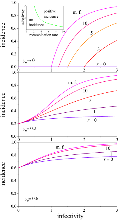
Figure 2: SIR epidemics incidence as a function of the infectivity for three initial fractions of infectious agents, $y_{0}$, and several recombination rates, $r$. Mean field (m. f.) results are also shown. The insert in the upper panel displays the boundary between the phases of no incidence and positive incidence for $y_{0}\to 0$, in the parameter plane of infectivity vs. recombination rate.

4 Numerical results for recombining couples

We solve Eqs. (3) by means of a standard fourth-order Runge-Kutta algorithm. The initial conditions are as in the preceding section, representing no R–agents and a fraction $y_{0}$ of I–agents. The disease incidence $z^{*}$ is estimated from the third equation of Eqs. (6), using the long-time numerical solutions for $m_{\rm RR}$, $m_{\rm SR}$, and $m_{\rm IR}$. In the range of parameters considered here, numerical integration up to time $t=1000$ was enough to get a satisfactory approach to asymptotic values.

Figure 2 shows the incidence as a function of infectivity for three values of the initial fraction of I–agents, $y_{0}\to 0$, $y_{0}=0.2$ and $0.6$, and several values of the recombination rate $r$. Numerically, the limit $y_{0}\to 0$ has been represented by taking $y_{0}=10^{-9}$. Within the plot resolution, smaller values of $y_{0}$ give identical results. Mean field (m. f.) results are also shown. As expected from the analytical results presented in the preceding section, positive values of $r$ give rise to incidences between those obtained for a static couple pattern ($r=0$) and for the mean field description. Note that substantial departure from the limit of static couples is only got for relatively large recombination rates, $r>1$, when at least one recombination per couple occurs in the typical time of recovery from the infection.

Among these results, the most interesting situation is that of a vanishingly small initial fraction of I–agents, $y_{0}\to 0$. Figure 3 shows, in this case, the epidemics incidence as a function of the recombination rate for several fixed infectivities. We recall that, for $y_{0}\to 0$, the mean field description predicts a transcritical bifurcation between zero and positive incidence at a critical infectivity $\lambda=1$, while in the absence of recombination the incidence is identically zero for all infectivities. Our numerical calculations show that, for sufficiently large values of $r$, the transition is still present, but the critical point depends on the recombination rate. As $r$ grows to infinity, the critical infectivity decreases approaching unity.

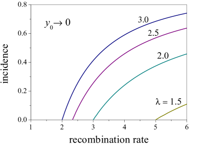
Figure 3: SIR epidemics incidence as a function of the recombination rate $r$ for a vanishingly small fraction of infectious agents, $y_{0}\to 0$, and several infectivities $\lambda$.

Straightforward linearization analysis of Eqs. (3) shows that the state of zero incidence becomes unstable above the critical infectivity

$$\lambda_{c}=\frac{r+1}{r-1}.$$ (9)

This value is in excellent agreement with the numerical determination of the transition point. Note also that Eq. (9) predicts a divergent critical infectivity for a recombination rate $r=1$. This implies that, for $0\leq r\leq 1$, the transition is absent and the disease has no incidence irrespectively of the infectivity level. For $y_{0}\to 0$, thus, the recombination rate must overcome the critical value $r_{c}=1$ to find positive incidence for sufficiently large infectivity. The critical line between zero and positive incidence in the parameter plane of infectivity vs. recombination rate, given by Eq. (9), is plotted in the insert of the upper panel of Fig. 2.

5 Conclusions

We have studied the dynamics of SIR epidemics in a population where, at any time, each agent forms a couple with exactly one neighbor, but neighbors are randomly exchanged at a fixed rate. As it had already been shown for the SIS epidemiological model [6, 7], this recombination of couples can, to some degree, compensate the high disconnection of the instantaneous interaction pattern, and thus allow for the propagation of the disease over a finite portion of the population. The interest of a separate study of SIR epidemics is based on its peculiar dynamical features: in contrast with SIS epidemics, it admits infinitely many absorbing equilibrium states. As a consequence, the disease incidence depends not only on the infectivity and the recombination rate, but also on the initial fraction of infectious agents in the population.

Due to the random nature of recombination, mean field–like arguments provide exact equations for the evolution of couples formed by agents in every possible epidemiological state. These equations can be analytically studied in the limits of zero and infinitely large recombination rates. The latter case, in particular, coincides with the standard mean field description of SIR epidemics.

Numerical solutions for intermediate recombination rates smoothly interpolate between the two limits, except when the initial fraction of infectious agents is vanishingly small. For this special situation, if the recombination rate is below one recombination event per couple per time unit (which equals the mean recovery time), the disease does not propagate and its incidence is thus equal to zero. Above that critical value, a transition appears as the disease infectivity changes: for small infectivities the incidence is still zero, while it becomes positive for large infectivities. The critical transition point shifts to lower infectivities as the recombination rate grows.

It is worth mentioning that a similar transition between a state with no disease and an endemic state with a permanent infection level occurs in SIS epidemics with a vanishingly small fraction of infectious agents [6, 7]. For this latter model, however, the transition is present for any positive recombination rate. For SIR epidemics, on the other hand, the recombination rate must overcome a critical value for the disease to spread, even at very large infectivities.

While both the (monogamous) structure and the (recombination) dynamics of the interaction pattern considered here are too artificial to play a role in the description of real systems, they correspond to significant limits of more realistic situations. First, the monogamous population represents the highest possible lack of connectivity in the interaction pattern (if isolated agents are excluded). Second, random couple recombination preserves the instantaneous structure of interactions and does not introduce correlations between the individual epidemiological state of agents. As was already demonstrated for SIS epidemics and chaotic synchronization [7], they have the additional advantage of being analytically tractable to a large extent. Therefore, this kind of assumption promises to become a useful tool in the study of dynamical processes on evolving networks.

- [1] R M Anderson, R M May, Infectious Diseases in Humans, Oxford University Press, Oxford (1991).
- [2] A S Mikhailov, Foundations of Synergetics I. Distributed active systems, Springer, Berlin (1990).
- [3] J D Murray, Mathematical Biology, Springer, Berlin (2003).
- [4] K T D Eames, M J Keeling, Modeling dynamic and network heterogeneities in the spread of sexually transmitted diseases, Proc. Nat. Acad. Sci. 99, 13330 (2002).
- [5] K T D Eames, M J Keeling, Monogamous networks and the spread of sexually transmitted diseases, Math. Biosc. 189, 115 (2004).
- [6] S Bouzat, D H Zanette, Sexually transmitted infections and the marriage problem, Eur. Phys. J B 70, 557 (2009).
- [7] F Vazquez, D H Zanette, Epidemics and chaotic synchronization in recombining monogamous populations, Physica D 239, 1922 (2010).
- [8] T Gross, C J Dommar D’Lima, B Blasius, Epidemic dynamics in an adaptive network, Phys. Rev. Lett. 96, 208 (2006).
- [9] T Gross, B Blasius, Adaptive coevolutionary networks: a review, J. R. Soc. Interface 5, 259 (2008).
- [10] D H Zanette, S Risau–Gusman, Infection spreading in a population with evolving contacts, J. Biol. Phys. 34, 135 (2008).
- [11] S Risau–Gusman, D H Zanette, Contact switching as a control strategy for epidemic outbreaks, J. Theor. Biol. 257, 52 (2009).