W+Jets at CDF: Evidence for Top Quarks

Abstract

Recently, an anomaly of $W$+jets events at large invariant masses has been reported by CDF. Many interpretations as physics beyond the Standard Model are being offered. We show how such an invariant mass peak can arise from a slight shift in the relative normalization of the top and $WW$ backgrounds.

In recent years, the Tevatron experiments have run a successful search program studying weak gauge boson and top quarks we well as searching for a Higgs boson and for new physics. A specific search for $V$+jets production $(V=W,Z)$ cdf_ww ; cdf_tc ; theo_wjets follows a long list of motivations review : we can test QCD effects such as the so-called staircase scaling of $n$-jet production theo_scaling , we can search for triple gauge boson couplings in $W^{+}W^{-}$ and $W^{\pm}Z$ production cdf_ww ; theo_ww , we can search for technicolor signals exis_tc ; theo_tc , or in the case of two bottom jets we can look for $WH$ associated production exis_wh . Some of these channels include a study of the invariant mass of the two leading jets recoiling against a leptonically decaying $W$ boson

$$p\bar{p}\to(W\to\ell\nu)\,+\text{2 jets}\,+X\qquad\qquad\qquad\qquad(\ell=\mu,e)$$ (1)

In their published study of $WV$ production based on an integrated luminosity of $3.9~{}{\rm fb^{-1}}$ and focused on an invariant mass regime $m_{jj}=50-130$ GeV the CDF collaboration has started to observe a slight excess of events in the region of $m_{jj}=150-180$ GeV cdf_ww . A D0 search based on the lower luminosity of $1.1~{}{\rm fb^{-1}}$ does not show any excess in this mass range d0_ww .

More recently, the CDF collaboration has published a dedicated study of the same anomaly cdf_tc with harder background rejection cuts and reports a $3.2~{}\sigma$ anomaly in the $m_{jj}$ spectrum. The excess is compatible with a resonance around 150 GeV. Many papers have since been published, explaining this observation, including technicolor bsm_tc , supersymmetric bsm_susy , lepto-phobic $Z^{\prime}$ boson bsm_zprime , color octets bsm_octet , and other interpretations bsm_other . In this paper we suggest an explanation of the excess based on a slight relative shift of the weight of different background contributions on the $WV$ pole an in the higher-mass region. While it is certainly possible to relieve the tension of the measurement and the background prediction for example by a shift in $m_{jj}$ or through the heavy flavor content of the proton, to our knowledge ours is the only way to explain the observed kinematic feature within the Standard Model.

A second peak from top decays

One of the backgrounds to $W$+jets production is the production of top quarks. Unlike to all other Standard Model channels, top quarks lead to a second peak in the $m_{jj}$ distribution, in addition to the $W$ mass peak. The angular correlation behind this second peak is between the bottom and the up-type quark $q_{\uparrow}$ from the $W$-decay. In the $W$ rest frame the distribution is given by

$$P(\cos\theta)=\frac{3}{8}\,\left(1+\cos\theta\right)^{2}\;F_{R}+\frac{3}{8}\,\left(1-\cos\theta\right)^{2}\;F_{L}+\frac{3}{4}\,\sin^{2}\theta F_{0}\;.$$ (2)

In the Standard Model the relative size of these contributions is $F_{0}:F_{L}:F_{R}\simeq 0.7:0.3:0$ top_kin . The corresponding invariant mass $m_{bq_{\uparrow}}$ is

$$P(m_{bq_{\uparrow}})=\frac{f_{R}(r)F_{R}+f_{L}(r)F_{L}+f_{0}(r)F_{0}}{m_{bj}^{\max}}\qquad\qquad\text{with}\quad r=\frac{m_{bq_{\uparrow}}}{m_{bj}^{\text{max}}}=\sqrt{\frac{1-\cos\theta}{2}}\;,$$ (3)

$f_{R}(r)=6r(1-r^{2})^{2}$, $f_{L}(r)=6r^{5}$, and $f_{0}(r)=12r^{3}(1-r^{2})$. Its upper endpoint is $m_{bj}^{\text{max}}=\sqrt{m_{t}^{2}-m_{W}^{2}}=154.6$ GeV, neglecting the bottom mass.

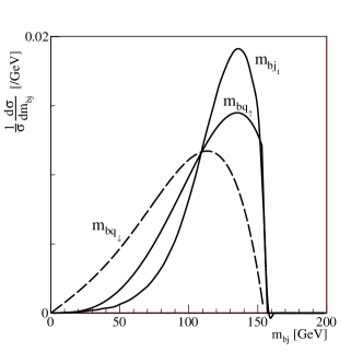
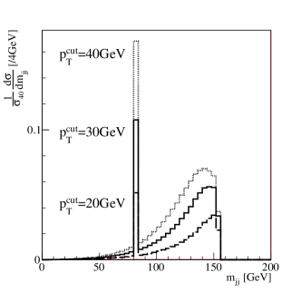
Figure 1: Left: theory predictions for the $m_{bq_{\uparrow}}$, $m_{bq_{\downarrow}}$ and $m_{bj_{1}}$ distributions at the parton level, simulated for top pair production. Right: $m_{j_{1}j_{2}}$ distribution with $p_{T,{j_{3}}}<20$ GeV (dashed), 30 GeV (solid) and 40 GeV (dotted).

The theory prediction for the $m_{bq_{\uparrow}}$ distribution we show in Fig. 1. Because of the left-handed $W$ interaction $m_{bq_{\uparrow}}$ gets contributions from $f_{L}$ and $f_{0}$; $m_{bq_{\downarrow}}$ corresponds to exchanging $f_{L}$ and $f_{R}$. Experimentally, we cannot distinguish between $q_{\uparrow}$ and $q_{\downarrow}$, so instead we define the invariant mass $m_{bj_{1}}$ with the harder of the two $W$ decay jets. This distribution is harder than $m_{bq_{\uparrow}}$. Without $b$ tagging the only observable distribution is $m_{j_{1}j_{2}}$, using the hardest two jets from the top decay. It shows a double peak structure from the sum of the $W$ peak and the $m_{bj_{1}}$ distribution. In Fig. 1 we also show how a stricter jet veto not only reduces the number of events but also produces a harder second peak in $m_{jj}$.

Loose cuts

In this first part of our paper we look at the original $WV$ analysis with the less significant but nevertheless clearly visible excess, shown in the left panel of Fig. 2 cdf_ww ; thesis . The basic acceptance and background rejection cuts are on one lepton and at least two jets plus missing transverse energy with

$$E_{T,\ell} >20~{}{\rm GeV}\qquad\qquad \hbox to0.0pt{\hbox to5.03125pt{\hfil/\hfil}\hss}p_{T} <25~{}{\rm GeV}\qquad\qquad M_{T,W} >30~{}{\rm GeV}$$

$$E_{T,j} >20~{}{\rm GeV}\qquad\qquad |\eta_{j}| <2.4\qquad\qquad |\Delta\phi_{\hbox to0.0pt{\hbox to3.52188pt{\hfil/\hfil}\hss}p_{T},j_{1}}| >0.4$$

$$p_{T,jj} >40~{}{\rm GeV}\qquad\qquad |\Delta\eta_{jj}| <2.5\;.$$ (4)

The main background is $W$+jets production with a variable normalization which can be fixed from the shape of the $m_{jj}$ distribution. This background shows essentially no structure. The second background is QCD jet production faking a lepton and missing transverse energy. For a $W$ decaying to an electron this background is about four times the size of the muon decay signature thesis . Again, this background has no visible structure in $m_{jj}$.

Of roughly similar size is the top background, consisting of top pairs and of single top production. As discussed above, this background has a distinct shape, namely two peaks including a Jacobian peak around 140 GeV. We see this shape in the right panel of Fig. 2. The peak arises if we combine the $b$ jet with one of the two light-flavor jets from the $W$ decay, which means it gets contributions from top pair production and from single top production with a $W$ boson. In the analysis, this background is normalized to the theory predictions $\sigma_{t\bar{t}}=7.5$ pb and $\sigma_{\text{single}\,t}=2.9$ pb theo_tops . The signal in this analysis is $WV$ production. It has a clear peak dominated by $W^{+}W^{-}$ production at $m_{jj}=80$ GeV, smeared by the experimental resolution. Its extracted rate, corrected to the total cross section without any detector effects or branching ratios is $13.5\pm 4.4$ pb for electrons and $23.5\pm 4.9$ pb for muons. In combination this gives $18.1\pm 3.3(\text{stat})\pm 2.5(\text{syst})$ pb. This combined number is compatible with the theory prediction.

However, the two significantly different results for the electron and the muon analyses with their different background compositions mostly in the $Z$+jets and QCD jets channels raise the question how well we actually know the total composition of all backgrounds. For backgrounds which do not have a distinct $m_{jj}$ shape this question is not very relevant, but for the top background and the $WV$ signal it matters. In the right panel of Fig. 2 we first show the individual templates for the top background and for the $WV$ channel. Our simulation is based on Alpgen alpgen + Pythia pythia at the particle level. To model the measured $m_{jj}$ distribution we apply a Gaussian smearing. Our template $m_{jj}$ distributions reproduce the CDF results thesis . The normalization we fix to the $4.3~{}{\rm fb^{-1}}$ of Ref. thesis , to properly take into account detector effects and efficiencies. This means that whenever we discuss the normalization of different cross sections we refer to the total rate after efficiencies and detector effects.

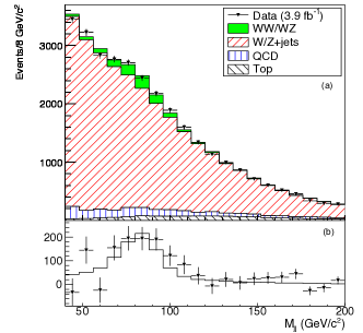
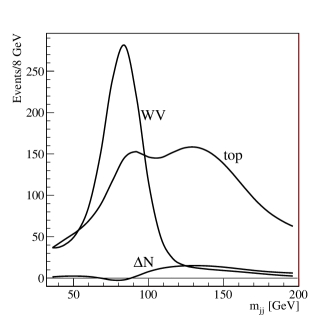
Figure 2: Left: excess in the $m_{jj}$ distribution above the $WV$ peak, as reported by CDF cdf_ww . The electron and muon decay channels are added. Right: $m_{jj}$ templates for the $WV$ and top samples individually. The normalization is chosen to match the CDF data. We also show the difference between the two samples for a 10% change of $\sigma_{\text{top}}$ and a corresponding shift in $\sigma_{WV}$, as described in the text.

The difference between the two templates becomes relevant if we change the relative contributions of the top and $WV$ backgrounds. The difference clearly matches the slight observed excess. To quantify this effect we compute the change in event numbers associated with a shift of the integrated rate or efficiency. We independently consider the peak region and the high mass regime

$$\Delta N_{[64,96]} =\;926\;\frac{\Delta\sigma_{WV}}{\sigma_{WV}} + \;542\;\frac{\Delta\sigma_{\text{top}}}{\sigma_{\text{top}}}$$

$$\Delta N_{[120,170]} =\;88\;\frac{\Delta\sigma_{WV}}{\sigma_{WV}} + \;915\;\frac{\Delta\sigma_{\text{top}}}{\sigma_{\text{top}}}\;.$$ (5)

These event numbers correspond to the CDF analysis thesis . Requiring that the sensitive normalization of the $WV$ mass peak $m_{jj}=64-96$ GeV be unchanged relates the two shifts as $(\Delta\sigma_{WV})/\sigma_{WV}=-0.59\,(\Delta\sigma_{\text{top}})/\sigma_{\text{top}}$, assuming efficiencies do not vastly vary between the two mass windows. Using this relation we find a net shift in the high mass region

$$\Delta N_{[120,170]}=\;863\;\frac{\Delta\sigma_{\text{top}}}{\sigma_{\text{top}}}\;.$$ (6)

Throughout this paper $\sigma$ really means the cross section after cuts and efficiencies, i.e.  $\sigma\times\epsilon_{\text{cuts}}\times\epsilon_{\text{rec}}$. The shape of the difference we show in Fig. 2 for $(\Delta\sigma_{\text{top}})/\sigma_{\text{top}}=10\%$. The experimentally observed excess for the loose set of cuts has the same shape. In Fig. 2 the mass window $m_{jj}=120-170$ GeV includes roughly 100 events which usually are attributed to the $WV$ contribution and any kind of new physics. If we conservatively neglect possible $WV$ contributions, according to Eq.(6) this corresponds to an $\mathcal{O}(10\%)$ shift in the combined top rate.

For the sum of top pairs and single top production with its different hard processes this shift could arise from a combination of experimental efficiencies and distributions mostly of the many jets involved. For example, the number of events which we expect from the combined top sample is very sensitive to the $p_{T,j}$ requirements we apply. Moreover, from the CDF publications cdf_ww ; thesis it is not clear how exactly the $tW$ single top channel has been computed pdf . Its size before cuts ranges around 1% of the top pair cross section single_top , but after the cuts Eq.(4) it could well account for a larger fraction of the shift in relative normalization.

The compensating shift in the $WV$ rate is even smaller and clearly within the sizable uncertainties of up to $\mathcal{O}(30\%)$ for the individual decay channels. In short, a very slight shift of the top sample normalization after cuts and efficiencies compensated for by a shift of the $WV$ rate completely explains the observed high-$m_{jj}$ anomaly. We should, however, remark that this loose cuts analysis is not a serious challenge to Standard Model explanations. It only serves as a way to illustrate and check our approach before we apply it to the more challenging dedicated analysis cdf_tc .

Hard cuts

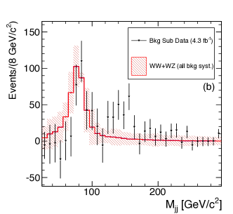
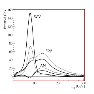
Figure 3: Left: excess in the $m_{jj}$ distribution above the $WV$ peak, as reported by CDF cdf_tc . The electron and muon decay channels are added. Right: $m_{jj}$ templates for the $WV$ and top samples individually. The dark lines assume $E_{T,j}=30$ GeV for the jet criteria, the lighter lines 40 GeV. We also show the difference between the two samples for a 40% change of $\sigma_{\text{top}}$ and a corresponding shift in $\sigma_{WV}$, as described in the text.

After observing the $m_{jj}$ anomaly in their $WV$ analysis CDF performed a dedicated analysis of this shape. To focus on the high-mass regime and to remove backgrounds they change some of the cuts shown in Eq.(4) to

$$\text{(1) exactly two jets with}\;E_{T,j} >30~{}{\rm GeV}\qquad\qquad\qquad\qquad\text{(2) additional dilepton veto}\;.$$ (7)

As we will see later, the veto on three or more jets makes a big difference, both in the extraction of the signal and in the uncertainties on the background estimates. Unlike for the loose cuts this experimental analysis show a distinct excess in Fig. 3. The additional requirements affects the relative composition of all channels in the $m_{jj}=[28,200]$ GeV window thesis . For example, $WV$ production now contributes 6.4% of all events, compared to 3.4% for the loose cuts. The top contribution very slightly decreases from 6.0% to 5.8%. For the two mass windows we now find

$$\Delta N_{[64,96]} =\;475\;\frac{\Delta\sigma_{WV}}{\sigma_{WV}} + \;137\;\frac{\Delta\sigma_{\text{top}}}{\sigma_{\text{top}}}$$

$$\Delta N_{[120,170]} =\;45\;\frac{\Delta\sigma_{WV}}{\sigma_{WV}} + \;244\;\frac{\Delta\sigma_{\text{top}}}{\sigma_{\text{top}}}.$$ (8)

Again, we use $\sigma$ for the cross section after cuts and efficiencies, i.e.  $\sigma\times\epsilon_{\text{cuts}}\times\epsilon_{\text{rec}}$. The relative normalization is fixed by the $WV$ peak region, giving us $(\Delta\sigma_{WV})/\sigma_{WV}=-0.29\,(\Delta\sigma_{\text{top}})/\sigma_{\text{top}}$ and

$$\Delta N_{[120,170]}=\;231\;\frac{\Delta\sigma_{\text{top}}}{\sigma_{\text{top}}}\;.$$ (9)

Naively, we see around 230 events in the high mass region $m_{jj}=120-170$ GeV. From this number we have to subtract the number of events which are described by the $WV$ channel, including systematic uncertainties. This leaves us with around 150 events which can for example be explained by a Gaussian new physics contribution.

However, this number of events changes after a more careful study of the $m_{jj}$ distribution. First, in the $m_{jj}=170-250$ GeV range we see a significant tail, consistently 10 to 20 events above the $WV$ expectations. They might be explained by some kind of continuous background which would also contribute to the $m_{jj}=170-250$ GeV window. Secondly, under the $WV$ peak of Fig. 3 there are clearly events missing, of the order of 50. Our simple compensation of the $WV$ and top channels cannot account for them because they are missing in the left side of the peak. Standard Model channels which rapidly drop towards larger $m_{jj}$ values should help explaining them. This way we would slightly decrease the number of events missing in the higher mass regime.

Nevertheless, explaining an excess of more than 100 events in the $m_{jj}=120-170$ GeV requires a sizable shift in the normalization of the top sample. Eq.(9) implies $\Delta\sigma_{\text{top}}\gtrsim 0.43\,\sigma_{\text{top}}$ and a compensating shift in the $WV$ rate of the order of $\mathcal{O}(10\%)$.

Of course, this does not mean a $43\%$ shift in the theoretically predicted total cross section for top production. Almost a third of the the combined top sample is single top production. For the jet veto survival probability the CDF analysis includes neither a reliable experimental cdf_single nor a reliable theoretical estimate single_top . Thus, we expect a very large error bar on the single top rate after cuts and efficiencies. Top pair production might not be quite as critical because the parton shower approximation should describe jets properly skands ; theo_scaling .

All efficiencies very strongly depend on the detailed simulation of the QCD jet activity and the $p_{T}$ requirements. For example, if we increase the detection and veto threshold from 30 GeV to 40 GeV the over-all efficiency increases quite dramatically for the top sample, as shown in Fig. 3 and expected from Fig. 1. In addition, it changes the shape of the top template. A reduced efficiency for $WV$ events means that instead of Eq.(9) we find $(\Delta\sigma_{WV}/\sigma_{WV})=-0.68\,(\Delta\sigma_{\text{top}})/\sigma_{\text{top}}$ and makes it easier to explain the second peak. This indicates large theory and systematic uncertainties associated with the jet veto. The fact that it is challenging to describe the top sample after jet related cuts is illustrated by the poor separation of different single top channels in the corresponding CDF analysis cdf_single . We check that the corresponding uncertainty for loose cuts without a jet veto is very well under control.

Taking our 40 GeV templates at face value the required change in the combined top rate drops significantly, entirely due to a strong dependence on the poorly understood jet veto survival probability. In essence, subtracting combined top backgrounds after a jet veto combines too many caveats which have to be taken into account as correspondingly large systematic and theoretical uncertainties.

Summary

We have shown that the apparent excess in $W$+jet events can be explained by Standard Model top backgrounds. Hadronically decaying top quarks generically produce two peaks in the $m_{jj}$ distribution. To explain the CDF measurements we have to enhance the normalization of the combined top pair and single top templates after cuts and detector efficiencies. Given the inherent difficulties in quantifying jet veto survival probabilities, such a shift in the $10\%$ (for the $WW$ analysis without a jet veto) or the $40\%$ (for the high-mass analysis with a jet veto) range appears reasonable and expected from QCD considerations. To maintain the measured event numbers under the $WW$ peak we compensate for this shift in the top template with another shift in the $WW$ normalization. The latter does not exceed 10% and is well within the uncertainties indicated by the different CDF results for the individual electron and muon channels.

Note added: after this work was finished, another paper with very similar conclusions appeared zack .

References

- (1) T. Aaltonen et al. [CDF Collaboration], Phys. Rev. Lett. 104, 101801 (2010) [arXiv:0911.4449 [hep-ex]].
- (2) T. Aaltonen et al. [CDF Collaboration], arXiv:1104.0699 [hep-ex].
- (3) M. L. Mangano, S. J. Parke, Phys. Rev. D41, 59-64 (1990); J. M. Campbell, R. K. Ellis, Phys. Rev. D65, 113007 (2002); J. M. Campbell, R. K. Ellis, D. L. Rainwater, Phys. Rev. D68, 094021 (2003); R. K. Ellis, K. Melnikov, G. Zanderighi, JHEP 0904, 077 (2009); C. F. Berger et al., Phys. Rev. Lett. 106, 092001 (2011).
- (4) D. E. Morrissey, T. Plehn and T. M. P. Tait, arXiv:0912.3259 [hep-ph].
- (5) see e.g. S. D. Ellis, R. Kleiss, W. J. Stirling, Phys. Lett. B154, 435 (1985); C. Englert, T. Plehn, P. Schichtel, S. Schumann, [arXiv:1102.4615 [hep-ph]].
- (6) see e.g. J. M. Campbell, R. K. Ellis, Phys. Rev. D60, 113006 (1999).
- (7) S. Mrenna, J. Womersley, Phys. Lett. B451, 155-160 (1999).
- (8) see e.g. C. T. Hill, E. H. Simmons, Phys. Rept. 381, 235-402 (2003).
- (9) M. S. Carena et al. [ Higgs Working Group Collaboration ], [hep-ph/0010338].
- (10) V. M. Abazov et al. [D0 Collaboration], Phys. Rev. D 80, 053012 (2009).
- (11) E. J. Eichten, K. Lane, A. Martin, [arXiv:1104.0976 [hep-ph]].
- (12) R. Sato, S. Shirai and K. Yonekura, arXiv:1104.2014 [hep-ph].
- (13) M. R. Buckley, D. Hooper, J. Kopp, E. Neil, [arXiv:1103.6035 [hep-ph]]; F. Yu, arXiv:1104.0243 [hep-ph]; K. Cheung and J. Song, arXiv:1104.1375 [hep-ph]; L. A. Anchordoqui, H. Goldberg, X. Huang, D. Lüst and T. R. Taylor, arXiv:1104.2302 [hep-ph]; M. Buckley, P. F. Perez, D. Hooper and E. Neil, arXiv:1104.3145 [hep-ph].
- (14) X. P. Wang, Y. K. Wang, B. Xiao, J. Xu and S. h. Zhu, arXiv:1104.1917 [hep-ph]; B. A. Dobrescu and G. Z. Krnjaic, arXiv:1104.2893 [hep-ph].
- (15) C. Kilic and S. Thomas, arXiv:1104.1002 [hep-ph]; J. A. Aguilar-Saavedra and M. Perez-Victoria, arXiv:1104.1385 [hep-ph]; A. E. Nelson, T. Okui and T. S. Roy, arXiv:1104.2030 [hep-ph]; S. Jung, A. Pierce and J. D. Wells, arXiv:1104.3139 [hep-ph].
- (16) G. L. Kane, G. A. Ladinsky and C. P. Yuan, Phys. Rev. D 45, 124 (1992); M. M. Nojiri and M. Takeuchi, JHEP 0810, 025 (2008).
-
(17)
V. Cavaliere,
Fermilab Ph.D Thesis 2010-51,
www.slac.stanford.edu/spires/find/hep/www?r=FERMILAB-THESIS-2010-51. - (18) M. L. Mangano, M. Moretti, F. Piccinini, R. Pittau, A. D. Polosa, JHEP 0307, 001 (2003).
- (19) T. Sjostrand, S. Mrenna, P. Z. Skands, JHEP 0605, 026 (2006).
- (20) B. W. Harris, E. Laenen, L. Phaf, Z. Sullivan and S. Weinzierl, Phys. Rev. D 66, 054024 (2002); M. Cacciari, S. Frixione, M. L. Mangano, P. Nason and G. Ridolfi, JHEP 0809, 127 (2008).
- (21) see e.g. T. M. P. Tait, Phys. Rev. D61, 034001 (2000); Z. Sullivan, Phys. Rev. D70, 114012 (2004); Q. -H. Cao, R. Schwienhorst, C. -P. Yuan, Phys. Rev. D71, 054023 (2005); Q. -H. Cao, R. Schwienhorst, J. A. Benitez, R. Brock, C. -P. Yuan, Phys. Rev. D72, 094027 (2005); T. Plehn, M. Rauch, M. Spannowsky, Phys. Rev. D80, 114027 (2009); S. Alioli, P. Nason, C. Oleari, E. Re, JHEP 0909, 111 (2009).
- (22) X. G. He and B. Q. Ma, arXiv:1104.1894 [hep-ph].
- (23) T. Aaltonen et al. [CDF Collaboration], Phys. Rev. D 82, 112005 (2010).
- (24) T. Plehn, D. Rainwater, P. Z. Skands, Phys. Lett. B645, 217-221 (2007); T. Plehn, T. M. P. Tait, J. Phys. G G36, 075001 (2009); J. Alwall, S. de Visscher, F. Maltoni, JHEP 0902, 017 (2009).
- (25) Z. Sullivan and A. Menon, arXiv:1104.3790 [hep-ph].