$AdS_{5}\times S^{5}$ mirror TBA equations from Y-system and discontinuity relations

Abstract:

Using the recently proposed set of discontinuity relations we translate the AdS/CFT Y-system to TBA integral equations and quantization conditions for a large subset of excited states from the ${\mathfrak{sl}(2)}$ sector of the $AdS_{5}\times S^{5}$ string $\sigma$-model. Our derivation provides an analytic proof of the fact that the exact Bethe equations reduce to the Beisert-Staudacher equations in the asymptotic limit. We also construct the corresponding T-system and show that in the language of T-functions the energy formula reduces to a single term which depends on a single T-function.

1 Introduction

An important problem in the AdS/CFT correspondence [1] is the calculation of anomalous dimensions in the planar ${\cal{N}}=4$ super Yang-Mills theory (SYM) or equivalently the energies of the dual $AdS_{5}\times S^{5}$ string sigma-model.

The integrability discovered on both sides of the correspondence provided us with an efficient mathematical apparatus to compute the exact spectrum of the planar AdS/CFT models. As the central object of integrability the 2-particle S-matrix of the model [3, 4, 5] plays a prominent role and is indispensable for the methods which enable us to compute the exact spectrum.

First, the spectrum of long operators or equivalently states with large R-charge $J$ was determined by the asymptotic Bethe Ansatz (ABA) [6, 7], which describes all polynomial corrections in $1/J$.

Later, the leading exponentially small corrections in $J$ could be taken into account by means of the generalized Lüscher formulae [9, 10, 11]. For the Konishi field their small coupling expansion led to beautiful agreement with direct 4-loop field theoretical computations [12, 13]. For a certain class of states in the ${\mathfrak{sl}(2)}$ sector the 4- and 5-loop expansion of these formulae [14, 15, 16] also satisfy nontrivial consistency checks dictated by perturbation theory considerations in the planar ${\cal{N}}=4$ SYM [17, 18].

The exact energies, which resum all wrapping corrections in $J$, can be obtained by the application of the Thermodynamic Bethe Ansatz method [19] to the doubly Wick rotated $AdS_{5}\times S^{5}$ string sigma-model called the mirror model [20, 21].

Strictly speaking the TBA method provides only the ground state energy of the model in finite volume and its extension to excited states is only a conjecture even if in most of the cases it rests on solid grounds. Based on the corresponding string-hypothesis [22] the ground state TBA equations of the $AdS_{5}\times S^{5}$ mirror model were constructed in [23, 24, 25] and simplified in [26]. In AdS/CFT the ground state TBA equations do not give much information about the spectrum since the ground state is protected by supersymmetry, i.e. $E_{0}(L)=0$.

The ground state equations are important nevertheless because they serve as starting point for the excited state equations. An important further discovery is that the Y-functions of the mirror TBA equations satisfy the so called Y-system functional equations [27]. The Y-functions can be rephrased in the language of T-functions satisfying the so-called T-system. The T-system of AdS/CFT lives on a T-hook [27]. The discovery of the Y- and T-systems (see Figs. 1, 2) made it possible to determine the asymptotic (large $J$) solutions of the excited state TBA problem. The asymptotic solution is constructed so that the ABA and the generalized Lüscher formulae are reproduced.

Based on previously elaborated examples in lattice models [28, 29] and in relativistic quantum field theory (QFT) [30, 31, 32, 33], the common experience is that excited state TBA equations differ from the ground state ones only in source terms and in quantization conditions imposed on objects appearing in the arguments of these terms. These source terms can be found by various methods like analytic continuation in some parameter of the model [30], deforming the integration contour of the ground state equations [28, 34] or transforming the Y-system functional relations to integral equations [28, 29, 32, 33]. In AdS/CFT the analytic continuation [24, 35] and contour deformation [34] methods together with requiring consistency with the large $J$ asymptotic solution were successfully applied to find the excited state TBA equations for certain states of the ${\mathfrak{sl}(2)}$ sector of the model. In [36] a general strategy to construct the TBA equations for all states of the model by the contour deformation method is outlined.

Since the TBA equations in AdS/CFT still cannot be derived from first principles it is important to test them carefully. In the strong coupling limit it was shown [37, 38] that the TBA equations reproduce the 1-loop string energies in the semi-classical limit and the strong coupling expansion of the energy of the Konishi state fitted from numerical TBA computations [35, 39] was found to be consistent with direct string theory computations [40]. At weak coupling 5-loop TBA results for the twist-2 states agree [41, 42, 43] with those based on the generalized Lüscher formula.

Though the analytic continuation and contour deformation methods provide the TBA equations for excited states it is important to derive the TBA equations from the Y-system functional relations as well. The main advantage of the Y-system based method is that the infinite Y-system can be solved via the T-system and the related T-Q relations, thus it opens the way towards the NLIE formulation of the AdS/CFT spectral problem.

However, until ref. [44] appeared, the Y-system based derivation of the TBA equations was impossible because the Y-functions are not meromorphic functions like in the relativistic models and have nontrivial discontinuity structure. The main discovery of ref. [44] was that this extra difficulty can be overcome for the ground state if the Y-system equations are supplemented by appropriate functional relations for the square-root discontinuities of the Y-functions. The Y-system equations supplemented by the discontinuity functional relations plus some analyticity assumption on the distribution of zeroes and poles of the Y-functions are sufficient to transform the Y-system to TBA integral equations. In this spirit the ground state TBA equations (including the dressing kernel) were derived [44] assuming that none of the Y-functions have local singularities in the entire complex plane.

It was conjectured in ref. [44] that the form of the discontinuity functional relations is state independent. If true, this allows us to derive excited state TBA equations from the Y-system as well. In this paper we carry out the Y-system based derivation of the excited state TBA equations. We consider states consisting of fundamental particles only, i.e. we assume all particle rapidities are real. As a first step we have checked that the conjecture is true in the asymptotic limit and found that the asymptotic solutions given in appendix C satisfy the discontinuity relations nontrivially.

Furthermore we show that we do not need to know the “local” analyticity properties of the Y-functions in the entire complex plane, it is sufficient to know their behaviour in certain regions near the real line. This means that the assumption of ref. [44] concerning the “local” singularities of the ground state Y-functions is too restrictive. Indeed, in [45] it has been shown numerically that the ground state Y-functions do have local singularities in the complex plane. Reconsidering the derivation it turned out that the local singularities are arranged in “complexes” (see ref. [45]), lie outside the physical strip and do not modify the form of the TBA equations.

Throughout the paper we assume that within certain regions of the complex plane the excited state Y-functions are smooth deformations of the asymptotic solution given in [27]. More precisely, we only discuss that part of the parameter space where the exact solution has (qualitatively) the same analytic properties as the corresponding asymptotic solution. In practice, if the size of the system ($J$) together with other quantum numbers are fixed, this is realized for small enough coupling $g$. For larger $g$ the TBA equations for the given state may undergo phase transitions similarly to what was found in [34, 39]. In this paper we restrict our attention to the form of the TBA equations valid in the vicinity of the asymptotic solution. Then assuming that the solution of the Y-system is found we construct the T-functions in an appropriate gauge. These T-functions are also smooth deformations of their asymptotic forms.

The benefit of introducing the T-functions is 2-fold. On the one hand they serve as internal variables in terms of which the discontinuity relations and the derivation of the TBA equations simplifies drastically. On the other hand T-functions seem to be more fundamental objects from the point of view of the AdS/CFT spectral problem. For example we show that the complicated TBA energy formula becomes a very simple expression containing the single T-function $T_{1,0}$. This fact indicates that there is an integrable $psu(2,2|4)$ spin-chain in the background such that the Hamiltonian is related to a transfer matrix of the model similarly to the cases of lattice models and lattice regularizations [46] of integrable QFTs [47, 48] studied previuosly.

Our final equations agree with previous results of [34]. Our derivation is based on functional relations and analyticity assumptions which we know are satisfied exactly in the asymptotic limit. Hence as a by-product our results prove analytically that the asymptotic solution satisfies the large $J$ limit of the TBA equations and also that the large $J$ limit of the exact Bethe equations coincide with the ABA equations. This fact, although it played an important role in the extraction of the 5-loop Lüscher terms from TBA [41, 42, 43], has not been proven analytically so far.

The organization of the paper is as follows. In the next section we introduce our starting relations and assumptions. Section 3 contains important lemmas and the transformation of the Y-system to TBA integral equations leaving the necessary discontinuities temporarily unspecified. In section 4 we construct the T-system in a partially fixed special gauge which turns out to be very useful to simplify the derivation of the TBA equations. In section 5 and 6 we compute the so far undetermined discontinuities $Y_{-}^{(\alpha)}/Y_{+}^{(\alpha)}$ and $\Delta$ from dispersion relations and we fix completely our gauge choice for the T-functions. In section 7 we derive the simplified version of the TBA equations, while section 8 contains their canonical and hybrid form. In section 9 we discuss the quantization conditions and the exact Bethe equations. Finally, in section 10 we discuss a simplified energy formula. The paper is closed by our conclusions. Appendix A contains the definitions of frequently used objects and kernels, appendix B the discussion of the branch cut discontinuities of the dressing part of the discontinuity function $\Delta$. In appendix C the asymptotic solution of the Y- and T-system equations are presented, in appendix D the precise definition of the discontinuity relations is given and finally in appendix E we discuss the meaning of the exact Bethe quantization conditions.

2 Starting relations and assumptions

Our starting point in this paper is the hypothesis that the same Y-system describes all excited states in the planar AdS/CFT spectral problem [27]. The Y-system of AdS/CFT takes the standard form

$$Y_{a,s}^{+}\,Y_{a,s}^{-}=\frac{(1+Y_{a,s-1})\,(1+Y_{a,s+1})}{(1+1/{Y_{a-1,s}})\,(1+1/{Y_{a+1,s}})},$$ (1)

but it lives on an $(a,s)$ lattice represented in Fig. 1. This is equivalent to imposing the boundary conditions $Y_{0,s}\to\infty$, $Y_{2,|s|>2}\to\infty$ and $Y_{a>2,\pm 2}\to 0$ while the product $Y_{3,\pm 2}\,Y_{2,\pm 3}$ should be kept finite in order to $Y_{2,\pm 2}$ be finite. This last requirement shows that the Y-system defined in the domain of Fig. 1 cannot form a closed set of equations because the new functions $Y_{3,\pm 2}\,Y_{2,\pm 3}$ enter the problem and we need additional equations (independent of the Y-system) to complete the system.

The Y-system is equivalent to a T-system defined on a T-hook of Fig. 2:

$$T_{a,s}^{+}\,T_{a,s}^{-}=T_{a+1,s}\,T_{a-1,s}+T_{a,s+1}\,T_{a,s-1},$$ (2)

where the relation to the $Y_{a,s}$ functions is given by

$$Y_{a,s}=\frac{T_{a,s+1}\,T_{a,s-1}}{T_{a+1,s}\,T_{a-1,s}},\qquad 1+Y_{a,s}=\frac{T_{a,s}^{+}\,T_{a,s}^{-}}{T_{a+1,s}\,T_{a-1,s}},\qquad 1+1/Y_{a,s}=\frac{T_{a,s}^{+}\,T_{a,s}^{-}}{T_{a,s-1}\,T_{a,s+1}}.$$ (3)

The T-equations can be extended to the infinite $(a,s)$ lattice by imposing the boundary conditions that all $T_{a,s}=0$ outside the T-hook. The T-system is a more fundamental set of equations than the Y-system because it forms a closed set of functional equations which determines all the Y-functions together with the supplementary combination $Y_{3,\pm 2}\,Y_{2,\pm 3}$. The T-equations and the Y-functions given by (3) are invariant with respect to the gauge transformations

$$T_{a,s}\rightarrow g_{1}^{[a+s]}\,g_{2}^{[a-s]}\,g_{3}^{[s-a]}\,g_{4}^{[-s-a]}\,T_{a,s},$$ (4)

with $g_{1,2,3,4}$ being arbitrary functions. In this paper we will choose a gauge where $T_{0,s}=1$. This fixes $g_{1}g_{3}=g_{2}g_{4}=1$.

It is known that in AdS/CFT the Y-functions have square root branch cuts and live on an infinite genus Riemann surface [25, 26, 44, 49]. The different sheets of the Riemann surface are connected through square-root branch cuts starting from the branch points with real parts $\pm 2$ and run to infinity along the lines with integer (in $1/g$ units) imaginary parts. To avoid the complications connected to using different sheets we will use a convention where all our functions are assumed to be defined on the first Riemann sheet, defined as the entire complex plane excluding the above cuts. In our convention if we analytically continue a function through one of the cuts, this becomes a new function, which can also be continued to the entire first Riemann sheet. We will often use the operation $f(u)\rightarrow f_{*}(u)$ corresponding to analytic continuation of the function $f(u)$ through the real cut $|u|\geq 2$. The construction of $f_{*}(u)$ consists of the two steps of analytic continuation of $f(u)$ through the real cut followed by analytic extension of the new function to the entire first Riemann sheet. Our functions are assumed to be meromorphic in the first Riemann sheet: they have discontinuities along some (but not necessarily all) of the cuts of the first Riemann sheet and cannot have other discontinuities but may have local singularities (zeroes and/or poles) in the sheet (and in some cases even on the cuts).

Restricting the Y-functions to the first Riemann sheet the Y-system equations supplemented by some analyticity information on the local singularities are not enough to derive the TBA integral equations. Some additional information on the discontinuities is needed as well. According to the proposal of ref. [44] this missing piece of information is a set of functional equations relating the discontinuities in a state independent way. These discontinuity equations translated to dispersion relations determine the extra $Y_{3,2}\,Y_{2,3}$ functions as well.

We will use the conventions of ref. [34] throughout the paper. The Y-functions in these conventions are related to the $Y_{a,s}$ variables as follows:

$$Y_{-}^{(\alpha)}=-1/Y_{1,\alpha 1},\qquad Y_{+}^{(\alpha)}=-Y_{2,\alpha 2},\quad\alpha=\pm\qquad Y_{Q}=Y_{Q,0}\quad\quad Q=1,2,...$$ (5)

$$Y_{m|vw}^{(\alpha)}=1/Y_{m+1,\alpha 1}\qquad Y_{m|w}^{(\alpha)}=Y_{1,\alpha(m+1)}\qquad\alpha=\pm\quad m=1,2,...$$ (6)

From the ground state equations we obtain the following structure for the locations of the branch cuts:

• $Y_{\pm}^{(\alpha)}(u):\qquad u+i\,2\,m/g\quad\quad m\in\mathbb{Z}$,

• $Y_{m}(u),\quad Y_{m|vw}^{(\alpha)}(u),\quad Y_{m|w}^{(\alpha)}(u):\qquad u\pm i\,(m+2\,j)/g,\qquad j=1,2,...,\infty$,

where $u\in(-\infty,-2)\cup(2,\infty)$. One of our main assumptions is that this structure remains valid for the excited states as well. For later convenience we rewrite the discontinuity relations proposed in [44] for the square-root branch cuts in the conventions we are using in this paper. We introduce the symbol $[f]_{Z}$ with $Z\in\mathbb{Z}$ to denote the discontinuity of the function $f(u)$:

$$[f(u)]_{Z}=\lim_{\epsilon\to 0^{+}}\left(f(u+i\,Z/g+i\epsilon)-f(u+i\,Z/g-i\epsilon)\right),\qquad u\in(-\infty,-2)\cup(2,\infty)$$ (7)

and define

$$\Delta=[\ln Y_{1}]_{+1}.$$ (8)

The discontinuity relations relate the “jumps” of this function and those of some other Y-functions. They take the form

$$[\Delta]_{\pm 2N}=\pm\sum_{\alpha}\left(\left[\ln\!\left(1-\frac{1}{Y_{\mp}^{(\alpha)}}\right)\right]_{\pm 2N}\!+\sum\limits_{m=1}^{N}\,\left[\ln\!\left(1+\frac{1}{Y_{m|vw}^{(\alpha)}}\right)\right]_{\pm(2N-m)}\!\!\!\!\!\!\!\!+\!\ln\!\left(\frac{Y_{-}^{(\alpha)}}{Y_{+}^{(\alpha)}}\right)\right)$$ (9)

$$\left[\ln\!\left(\frac{Y_{-}^{(\alpha)}}{Y_{+}^{(\alpha)}}\right)\right]_{\pm 2N}=-\sum\limits_{Q=1}^{N}\,\left[\ln\!\left(1+Y_{Q}\right)\right]_{\pm(2N-Q)}$$ (10)

with $N=1,2,...$ and

$$\left[\ln\!Y_{1|vw}^{(\alpha)}\right]_{\pm 1}=\ln\!\left(\frac{1-Y_{-}^{(\alpha)}}{1-Y_{+}^{(\alpha)}}\right),\qquad\left[\ln\!Y_{1|w}^{(\alpha)}\right]_{\pm 1}=\ln\!\left(\frac{1-1/Y_{-}^{(\alpha)}}{1-1/Y_{+}^{(\alpha)}}\right).$$ (11)

In the sequel $[f(u)]_{Z}$ means the analytic extension of the discontinuity (7) to generic values of $u$. Using the notation defined earlier in this section we can write $[f(u)]_{Z}=f^{[+Z]}(u)-(f^{[+Z]})_{*}(u)$ where $(f^{[+Z]})_{*}(u)$ is the function obtained by analytic continuation of $(f^{[+Z]})(u)$ through the cut lying along the real line (crossing it from below) and then extended to the first Riemann sheet.

Some important remarks on the interpretation of the discontinuity relations (8-11) are in order. As they stand, (8-11) are valid if the Y-function combinations appearing in them have no logarithmic discontinuities crossing the lines of the square-root discontinuities. In order to get rid of the difficulties caused by the logarithmic discontinuities we use the derivative of the discontinuity relations (8-11) as our starting point and apply dispersion relations for the derivatives of $\Delta$ and $\ln Y_{-}^{(\alpha)}/Y_{+}^{(\alpha)}$. Then a second subtlety appears if there are local singularities of the Y-function combinations lying exactly on the lines of square-root discontinuities. Such local singularities do not modify the discontinuity relations, but they contribute to the corresponding dispersion relation through the residue theorem. To cure this problem a finer interpretation of the discontinuity relations is necessary in which the contribution of such local singularities are taken into account as well.

To find the correct interpretation we can invoke the asymptotic solution. It can be shown that only (9) at $N=1$ and at the positions of real poles of $1-1/Y_{\pm}^{(\alpha)}$ must be refined. The term which causes the trouble is $\left[\ln\left(1+{1}/{Y_{1|vw}^{(\alpha)}}\right)\right]_{\pm 1}$ on the right hand side of (9), because its derivative has poles sitting right on the discontinuities with $\mbox{Im}u=\pm 1/g$. This refined interpretation of (8-11) is necessary only when they are translated to dispersion relations. In order for the dispersion relation applied for the derivative of (9) give the correct formula for $\Delta$ the following replacement must be done on the right hand side of (9) at $N=1$:

$$\left[\ln\left(1+\frac{1}{Y_{1|vw}^{(\alpha)}(u)}\right)\right]_{\pm 1}\rightarrow\left[\ln\left\{\left(1+\frac{1}{Y_{1|vw}^{(\alpha)}(u)}\right)\frac{1}{p_{2}^{(\alpha)\mp}(u)}\right\}\right]_{\pm 1},$$ (12)

where $p_{2}^{(\alpha)}(u)$ is the polynomial having zeroes at the positions of the real zeroes of $Y_{-}^{(\alpha)}$ with absolute values larger than $2$. In other words the poles corresponding to the zeroes of $p_{2}^{(\alpha)}(u)$ must be ignored. For a proof of this formula for the most general state of the model see appendix D.

We note that as a consequence of the definition (8), and the fact that going around twice a square root branch point gives back the original function, we have the relation

$$\Delta(u)=-\Delta_{*}(u).$$ (13)

The Y-system (1) and the discontinuity relations (8-11) are not sufficient to derive the TBA equations. Some more information is needed about the discontinuities lying along the real axis. Based on the properties of the solution for the ground state TBA equations and the similar properties of the asymptotic solution for excited states, we require that the “fermionic” Y-functions $Y^{(\alpha)}_{\pm}$ are analytic continuations of each other:

$$Y_{-}^{(\alpha)}(u)=(Y_{+}^{(\alpha)})_{*}(u).$$ (14)

We will also assume that all Y-functions are real analytic. This assumption is based on the observations that the Y-functions are real analytic functions for the ground state solution of the TBA equations and also in the asymptotic limit for excited state solutions. Since we consider the AdS/CFT Y-functions as smooth deformations of their asymptotic counterparts we restrict ourselves to deformations that preserve the property of real analyticity. We note that in the absence of this assumption several TBA integral equations could be set up (such that their asymptotic limit coincides).

To summarize we assume that

• Y-functions satisfy the Y-system equations (1).

• The discontinuities are related by the modified relations (8-11),(12).

• $Y_{-}^{(\alpha)}(u)$ and $Y_{+}^{(\alpha)}(u)$ are related by (14).

• The Y-functions are real analytic functions.

• The Y-functions are smooth deformations of their asymptotic limit.

If one assumes that both $\Delta$ and $Y_{-}^{(\alpha)}/Y_{+}^{(\alpha)}$ are analytic and bounded near $\pm 2$ then their discontinuities must be zero at the branching points $\pm 2$. From this requirement and from (13), (14) it follows that the combinations $\Delta(u)/\sqrt{4-u^{2}}$ and $\ln(Y_{-}^{(\alpha)}/Y_{+}^{(\alpha)})/\sqrt{4-u^{2}}$ have no square root branch cuts along the real axis. These properties have been used in the derivation given in ref. [44] and we think it is important to emphasize them since they play very important role also in our considerations.

The form of the discontinuity relations (8-11) and (14) have been conjectured to be independent of the particular excited state of the $AdS_{5}\times S^{5}$ sigma-model under consideration. Using the formulae and results of appendices A, B, and C this conjecture can be proven to be valid for the asymptotic solutions. Here we will verify the relations (10),(11) and (14) in the asymptotic limit. The (asymptotic) justification of (9) will be presented in section 6.

With the help of the T-function representation of $Y_{-}^{(0)}/Y_{+}^{(0)}$ and the formulae of appendix C it can be shown that asymptotically:

$$\ln\left(Y_{-}^{(0)}/Y_{+}^{(0)}\right)=\ln\frac{R_{p}\,B_{m}}{R_{m}\,B_{p}},$$ (15)

from which $\left[\ln\left(Y_{-}^{(0)}/Y_{+}^{(0)}\right)\right]_{\pm 2N}=0$, the asymptotic $(Y_{Q}\to 0)$ limit of (10), follows immediately.

Next we write

$$\left(1-\frac{1}{Y^{(0)}_{-}}\right)_{*}=(1+Y_{1,1}^{(0)})_{*}=\frac{{\cal F}^{(0)+}{\cal G}^{(0)-}}{T_{2,1}^{(0)}}=\frac{T_{2,2}^{(0)+}T_{2,2}^{(0)-}}{T_{2,1}^{(0)}T_{2,3}^{(0)}}=1+\frac{1}{Y_{2,2}^{(0)}}=1-\frac{1}{Y_{+}^{(0)}},$$ (16)

where we have used the identity

$$T_{2,2}^{(0)+}\,T_{2,2}^{(0)-}={\cal F}^{(0)+}\,{\cal G}^{(0)-}T_{2,3}^{(0)}$$ (17)

and this proves (14) asymptotically.

The asymptotic verification of (11) goes as follows. Using the T-representation:

$$\left[\ln Y_{1|vw}^{(0)}\right]_{\pm 1}=-\left[\ln Y_{2,1}^{(0)}\right]_{\pm 1}=\left[\ln\frac{T_{1,1}^{(0)}}{T_{2,2}^{(0)}}\right]_{\pm 1}.$$ (18)

With the help of (327)-(335) it can be shown that:

$$\left[\ln\frac{T_{1,1}^{(0)}}{T_{2,2}^{(0)}}\right]_{\pm 1}=\ln\frac{T_{1,1}^{(0)+}\,T_{1,1}^{(0)-}}{{\cal F}^{(0)+}\,{\cal G}^{(0)-}}\frac{T_{3,2}^{(0)}}{T_{2,3}^{(0)}}=\ln\frac{1+1/Y_{1,1}^{(0)}}{1+Y_{2,2}^{(0)}}=\ln\frac{1-Y_{-}^{(0)}}{1-Y_{+}^{(0)}}.$$ (19)

Formulae (18) and (19) together verify the first relation of (11) while the second relation follows from (19) and the following two relations:

$$\left[\ln Y_{1|w}^{(0)}\right]_{\pm 1}=\left[\ln Y_{1,2}^{(0)}\right]_{\pm 1}=\left[\ln\frac{T_{1,1}^{(0)}}{T_{2,2}^{(0)}}\right]_{\pm 1}+\left[\ln T_{1,3}^{(0)}\right]_{\pm 1},$$ (20)

$$\left[\ln T_{1,3}^{(0)}\right]_{\pm 1}=\ln Y_{1,1}^{(0)}Y_{2,2}^{(0)}=\ln\frac{Y_{+}^{(0)}}{Y_{-}^{(0)}}.$$ (21)

In the derivation of the excited state TBA equations we can avoid the technical problems coming from dealing with branch cuts of the $\log$ functions if we first derive equations for the derivatives of the $\log Y$-functions. To this end we use the logarithmic derivative of the Y-system (1), and the derivative of the discontinuity relations (8-11), (13) and (14). Qualitative information about the local singularities of the Y-functions can be read off from their asymptotic form. Finally we integrate the equations for the derivatives.

In order to be able to extract the necessary analyticity information on the local singularities of the Y-functions we will make use of the assumption that the exact Y-functions are smooth deformations of the asymptotic ones. This however cannot be satisfied in the whole complex plane, but only in certain strips (similarity regions). We will show that analyticity information regarding the behavior of our functions in these strips are enough to derive the TBA equations and to determine the exact Y-functions.

The Y-functions are smooth deformations of their asymptotic counterparts as long as the $Y_{Q}^{(0)}$ functions are small. From (347) it follows that this condition is satisfied in the region ${{\Omega}}_{\varepsilon_{Q}}=\{u\in\mathbb{C}:\quad|\mbox{Im}\,u|<Q/g,\quad|u-u_{j}^{[\pm(Q-1)]}|>\varepsilon_{Q}\}$, where $\varepsilon_{Q}$ is a small but not infinitesimal positive parameter for $Q\geq 2$ and zero for $Q=1$. Then the Y-system equations (1) imply for the other Y-functions the following similarity regions:

• $Y_{Q}(u)\sim Y_{Q}^{(0)}(u)=Y_{Q,0}^{(0)}(u)\qquad\,u\in\Omega_{\varepsilon_{Q}},\qquad Q=1,2,...,$

• $Y_{m|vw}^{(\alpha)}(u)\sim Y_{m|vw}^{(\alpha)(0)}(u)=1/Y_{m+1,\alpha 1}^{(0)}(u)\qquad|\mbox{Im}\,u|<m/g,\qquad m=1,2,...,$

• $Y_{m|w}^{(\alpha)}(u)\sim Y_{m|w}^{(\alpha)(0)}(u)=Y_{1,\alpha(m+1)}^{(0)}(u)\qquad|\mbox{Im}\,u|<m/g,\qquad m=1,2,...,$

• $Y_{-}^{(\alpha)}(u)\sim Y_{-}^{(\alpha)(0)}(u)=-1/Y_{1,\alpha 1}^{(0)}(u),\qquad|\mbox{Im}\,u|<2/g,\qquad\alpha=\pm,$

• $Y_{+}^{(\alpha)}(u)\sim Y_{+}^{(\alpha)(0)}(u)=-Y_{2,\alpha 2}^{(0)}(u),\qquad|\mbox{Im}\,u|<2/g,\qquad\alpha=\pm.$

The discontinuity relations (8-11) simplify considerably in the language of T-functions. The complicated products of Y-functions in the argument of the $\log$ function become a product of a few T-functions only. In section 4 we will show that there is a particular choice for the gauge where the exact T-functions are smooth deformations of the asymptotic ones and due to their simple square-root branch cut structure the right hand sides of (8-11) simplify drastically.

Figure 1: The ${\rm AdS}_{5}{\rm/CFT}_{4}$ Y-system. Full circles on the $a$ axis correspond to massive nodes with $s=0$. The $s$ axis corresponds to nodes with $a=1$.

Figure 2: The ${\rm AdS}_{5}{\rm/CFT}_{4}$ T-system. The $s$ axis corresponds to nodes with $a=0$.

3 TBA equations with cuts

In this section we transform the Y-system equations (1) into TBA integral equations. This transformation is not as complete here as for the case of integrable relativistic models because of the presence of cuts (discontinuities) in the analytic extension of some of the Y-functions. The Y-system equations are of the universal form

$$y^{+}y^{-}={\cal R},$$ (22)

but the details of the corresponding integral equation depend on the analytic properties of the “unknown” function $y$.

3.1 TBA lemma 1a

Assume that the set of zeroes [poles] of $y(u)$ inside the physical strip ($-1/g<{\rm Im}\,u<1/g$) is $\{\xi_{j}\}$ $[\{\eta_{k}\}]$. We also assume that there may be discontinuities along the cuts with imaginary part $\frac{i}{g}$:

$$\frac{y(u+\frac{i}{g}+i\epsilon)}{y(u+\frac{i}{g}-i\epsilon)}={\rm e}^{V(u+i\epsilon)},\qquad|u|\geq 2,\qquad V(\pm 2)=0.$$ (23)

Further we assume the large $u$ asymptotic behaviour

$$y(u)\approx y_{0}\,u^{M_{0}},\qquad u\longrightarrow\infty$$ (24)

below the cut and

$$y(u)\approx y_{+}\,u^{M_{+}},\qquad u\longrightarrow\infty+\frac{i}{g}+i\epsilon$$ (25)

just above the cut. (If there is no discontinuity then of course $y_{0}=y_{+}$, $M_{0}=M_{+}$.) The Y-system equation (22) implies that ${\cal R}(u)$ behaves asymptotically as

$${\cal R}(u)\approx y_{+}y_{0}u^{M_{0}+M_{+}},\qquad u\longrightarrow\infty+i\epsilon.$$ (26)

The function

$$\tau(u)=\frac{\prod_{j}t(u-\xi_{j})}{\prod_{k}t(u-\eta_{k})},$$ (27)

where

$$t(u)=\tanh\frac{\pi gu}{4}$$ (28)

has the same zeroes [poles] (in the physical strip) as $y(u)$ and satisfies $\tau^{+}\tau^{-}=1$. Using this function and the universal TBA kernel function

$$s(u)=\frac{g}{4\cosh\frac{\pi gu}{2}}$$ (29)

the solution of (22) which has the analytic properties detailed above is

$$y={\rm sgn}(y_{0})\tau\exp\{\ln{\cal R}^{\epsilon}\star s-V^{\epsilon}\ \check{\star}\ s\}.$$ (30)

Here ${\cal R}^{\epsilon}(u)={\cal R}(u+i\epsilon)$ and $V^{\epsilon}(u)=V(u+i\epsilon)$ and this notation indicates that the integration contour in (30) goes just above the real line. Our definition of the log (ln) function is the standard one: we always assume that the cut of this function is along the negative real axis.

The result (30) can be proven directly by substituting this expression into the functional equation (22).

3.2 TBA lemma 1b

In one of the TBA equations the Y-function has no cuts near the physical strip but singular points right at its boundaries. In this case we assume again that the set of zeroes [poles] of $y(u)$ inside the physical strip is $\{\xi_{j}\}$ $[\{\eta_{k}\}]$ and further assume that the set of zeroes [poles] on the boundary of the physical strip is $\{z_{\alpha}\pm\frac{i}{g}\}$ $[\{w_{\beta}\pm\frac{i}{g}\}]$, where $z_{\alpha}$ $[w_{\beta}]$ are real. The large $u$ asymptotic behaviour is

$$y(u)\approx y_{0}\,u^{M_{0}},\qquad u\longrightarrow\infty.$$ (31)

The Y-system equation (22) implies that ${\cal R}(u)$ has double zeroes [poles] at $\{z_{\alpha}\}$ $[\{w_{\beta}\}]$ and behaves asymptotically as

$${\cal R}(u)\approx y_{0}^{2}u^{2M_{0}},\qquad u\longrightarrow\infty+i\epsilon.$$ (32)

In this case the solution of (22) with the right analytic properties is

$$y={\rm sgn}(y_{0})\tau\exp\{\ln{\cal R}\star s\}.$$ (33)

The result (33) can be proven directly because the logarithmic singularities (at $\{z_{\alpha}\}$ $[\{w_{\beta}\}]$ or at $\infty$) are integrable and do not invalidate the result.

3.3 TBA lemma 2

Let us now assume that the “unknown” function $y(u)$ has zeroes [poles] inside the physical strip as before, and in addition has (multiplicative) discontinuities along the real cuts:

$$\frac{y(u+i\epsilon)}{y(u-i\epsilon)}={\rm e}^{J(u+i\epsilon)},\qquad|u|\geq 2,\qquad J(\pm 2)=0.$$ (34)

We also assume $y(u)$ has constant asymptotics for large $u$: it approaches the constants $y_{+}[y_{-}]$ when $u\longrightarrow\infty$ just above [below] the real line. This implies

$${\rm e}^{J(u+i\epsilon)}\approx J_{\infty}=\frac{y_{+}}{y_{-}},\qquad{\cal R}(u)\approx y_{+}y_{-},\qquad u\longrightarrow\infty.$$ (35)

In this case the solution of (22) is

$$y={\rm sgn}(y_{+})\tau\exp\{\ln{\cal R}\star s+J^{\epsilon}\ \check{\star}\ s_{1}\},$$ (36)

where

$$s_{1}(u)=\frac{-ig}{4\sinh\left(\frac{\pi gu}{2}-i\epsilon\right)}.$$ (37)

3.4 TBA integral equations

Using the above two lemmas we now write down the set of TBA integral equations corresponding to the Y-system (1). First we spell out these equations using the notations of (5-6):

$$Y^{(\alpha)+}_{m|vw}\,Y^{(\alpha)-}_{m|vw} = \frac{(1+Y^{(\alpha)}_{m+1|vw})(1+Y^{(\alpha)}_{m-1|vw})}{(1+Y_{m+1})},\qquad\qquad m\geq 2,$$ (38)

$$Y^{(\alpha)+}_{1|vw}\,Y^{(\alpha)-}_{1|vw} = \frac{1-Y_{-}^{(\alpha)}}{1-Y_{+}^{(\alpha)}}\,\frac{(1+Y^{(\alpha)}_{2|vw})}{(1+Y_{2})},$$ (39)

$$Y^{(\alpha)+}_{m|w}\,Y^{(\alpha)-}_{m|w} = (1+Y^{(\alpha)}_{m+1|w})(1+Y^{(\alpha)}_{m-1|w}),\qquad\qquad m\geq 2,$$ (40)

$$Y^{(\alpha)+}_{1|w}\,Y^{(\alpha)-}_{1|w} = \frac{1-\frac{1}{Y_{-}^{(\alpha)}}}{1-\frac{1}{Y_{+}^{(\alpha)}}}\,(1+Y^{(\alpha)}_{2|w}),$$ (41)

$$Y^{+}_{Q}\,Y^{-}_{Q} = \frac{Y_{Q+1}\,Y_{Q-1}}{Y^{(+)}_{Q-1|vw}\,Y^{(-)}_{Q-1|vw}}\,\frac{(1+Y^{(+)}_{Q-1|vw})(1+Y^{(-)}_{Q-1|vw})}{(1+Y_{Q+1})(1+Y_{Q-1})},\quad\quad Q\geq 2,$$ (42)

$$Y^{+}_{1}\,Y^{-}_{1} = \frac{Y_{2}}{Y^{(+)}_{-}\,Y^{(-)}_{-}}\,\frac{(1-Y_{-}^{(+)})(1-Y_{-}^{(-)})}{1+Y_{2}},$$ (43)

$$Y_{-}^{(\alpha)+}\,Y_{-}^{(\alpha)-} = \frac{1+Y_{1|vw}^{(\alpha)}}{(1+Y_{1})(1+Y^{(\alpha)}_{1|w})}.$$ (44)

Using the notation $X$ for a general index, which can take the values ${\phantom{Y}}_{Q}$, ${\phantom{Y}}^{(\alpha)}_{m|vw}$, ${\phantom{Y}}^{(\alpha)}_{m|w}$ or ${\phantom{Y}}^{(\alpha)}_{\pm}$, and denoting the set of zeroes of $Y_{X}$ in the physical strip by $\{\xi_{X,j}\}$ and the set of its poles by $\{\eta_{X,k}\}$, finally the sign of $Y_{X}(u)$ in the limit $u\longrightarrow\infty+i\epsilon$ by $({\rm sgn})_{X}$, we define

$$t_{X}(u)=({\rm sgn})_{X}\,\left\{\frac{\prod_{j}t(u-\xi_{X,j})}{\prod_{k}t(u-\eta_{X,k})}\right\}.$$ (45)

From the discontinuity relations we see that we can use Lemma 1a with $V=0$ for the cases (38), (40) and if $Q\geq 3$ also for (42). Lemma 1b is used for (42) if $Q=2$. Further we have to use Lemma 1a

$${\rm for\ the\ }Y_{1|vw}^{(\alpha)}{\rm\ equation\ (\ref{Y1vw})\ with\ }V = \ln\left(\frac{1-Y_{-}^{(\alpha)}}{1-Y_{+}^{(\alpha)}}\right)\,$$

$${\rm for\ the\ }Y_{1|w}^{(\alpha)}{\rm\ equation\ (\ref{Y1w})\ with\ }V = \ln\left(\frac{1-\frac{1}{Y_{-}^{(\alpha)}}}{1-\frac{1}{Y_{+}^{(\alpha)}}}\right)\,$$

$${\rm for\ the\ }Y_{1}{\rm\ equation\ (\ref{Y1})\ with\ }V = \Delta\,$$

and finally Lemma 2 for the $Y_{-}^{(\alpha)}$ equation (44) with $J=J^{(\alpha)}$.

We find

$$Y^{(\alpha)}_{m|vw} = t^{(\alpha)}_{m|vw}\exp\left\{\ln\left[\frac{(1+Y^{(\alpha)}_{m+1|vw})(1+Y^{(\alpha)}_{m-1|vw})}{(1+Y_{m+1})}\right]\star s\right\},\qquad m\geq 2,$$ (46)

$$Y^{(\alpha)}_{1|vw} = t^{(\alpha)}_{1|vw}\exp\left\{\ln\left[\frac{(1+Y^{(\alpha)}_{2|vw})}{(1+Y_{2})}\right]\star s+\ln\left[\frac{1-Y_{-}^{(\alpha)}}{1-Y_{+}^{(\alpha)}}\right]\ \hat{\star}\ s\right\},$$ (47)

$$Y^{(\alpha)}_{m|w} = t^{(\alpha)}_{m|w}\exp\left\{\ln\left[(1+Y^{(\alpha)}_{m+1|w})(1+Y^{(\alpha)}_{m-1|w})\right]\star s\right\},\qquad m\geq 2,$$ (48)

$$\ Y^{(\alpha)}_{1|w} = t^{(\alpha)}_{1|w}\exp\left\{\ln\left[1+Y^{(\alpha)}_{2|w}\right]\star s+\ln\left[\frac{1-\frac{1}{Y_{-}^{(\alpha)}}}{1-\frac{1}{Y_{+}^{(\alpha)}}}\right]\ \hat{\star}\ s\right\}\,,$$ (49)

$$Y_{Q} = t_{Q}\exp\left\{\ln\left[\frac{Y_{Q+1}\,Y_{Q-1}(1+Y^{(+)}_{Q-1|vw})(1+Y^{(-)}_{Q-1|vw})}{Y^{(+)}_{Q-1|vw}Y^{(-)}_{Q-1|vw}(1+Y_{Q+1})(1+Y_{Q-1})}\right]\star s\right\},\quad Q\geq 2,$$ (50)

$$Y_{1} = t_{1}\exp\left\{\ln\left[\frac{Y_{2}}{Y^{(+)}_{-}\,Y^{(-)}_{-}}\,\frac{(1-Y_{-}^{(+)})(1-Y_{-}^{(-)})}{1+Y_{2}}\right]\star s-\Delta\ \check{\star}\ s\right\},$$ (51)

$$Y_{-}^{(\alpha)} = t_{-}^{(\alpha)}\exp\left\{\ln\left[\frac{1+Y_{1|vw}^{(\alpha)}}{(1+Y_{1})(1+Y^{(\alpha)}_{1|w})}\right]\star s+J^{(\alpha)}\ \check{\star}\ s_{1}\right\}.$$ (52)

There is no equation for $Y_{+}^{(\alpha)}$, but since it is the analytic continuation of $Y_{-}^{(\alpha)}$, the very definition of the discontinuity $J^{(\alpha)}$ can be written as

$$Y_{+}^{(\alpha)}=Y_{-}^{(\alpha)}\exp\left\{-J^{(\alpha)}\right\}.$$ (53)

The above set of TBA integral equations is incomplete yet, since the discontinuities $\Delta$ and $J^{(\alpha)}$ are undetermined. They will be obtained using dispersion relations in Section 6 and Section 5, respectively.

4 Construction of the T-system

In this section we start to construct a T-system from the Y-system. This is not unique because there is a gauge freedom in this transformation. Since our main assumption is that the exact Y-functions are (at least qualitatively) close to their asymptotic values given by the Bethe Ansatz solution and in our subsequent considerations the T-system plays an important role, we will choose a gauge in which also the T-system is close to the asymptotic solution. This will be achieved here only partially and the final, complete gauge fixing will be given in Section 6.

4.1 Chain lemma

Let us assume that we want to find the solution of the infinite system

$$\frac{\sigma_{a}^{+}\sigma_{a}^{-}}{\sigma_{a+1}\sigma_{a-1}}=\xi_{a},\qquad a=1,2,\dots,\qquad\sigma_{0}\equiv 1,$$ (54)

where the unknowns $\sigma_{a}(u)$ are assumed to have no zeroes/poles near the physical strip (in the physical strip and a little beyond). $\xi_{a}(u)$ on the right hand side are given functions not having zeroes/poles near the real axis and taking complex values (excluding the negative real axis). Furthermore, (only) $\xi_{1}$ may have discontinuities on the real axis:

$$\frac{\xi_{1}(u+i\epsilon)}{\xi_{1}(u-i\epsilon)}={\rm e}^{I(u+i\epsilon)},\qquad I(\pm 2)=0.$$ (55)

In such a case we assume that (only) $\sigma_{1}$ has discontinuities along the cuts with imaginary part $\pm\frac{i}{g}$:

$$\frac{\sigma_{1}(u+\frac{i}{g}+i\epsilon)}{\sigma_{1}(u+\frac{i}{g}-i\epsilon)}={\rm e}^{p(u+i\epsilon)},\qquad\quad\frac{\sigma_{1}(u-\frac{i}{g}+i\epsilon)}{\sigma_{1}(u-\frac{i}{g}-i\epsilon)}={\rm e}^{m(u+i\epsilon)},$$ (56)

where

$$p+m=I,\qquad\quad p(\pm 2)=m(\pm 2)=0.$$ (57)

The solution of (54) is given by

$$\sigma_{a}=\exp\left\{\sum_{A=1}^{\infty}\ln\xi_{A}^{\epsilon}\star\ell^{A}_{a}-p^{\epsilon}\ \check{\star}\ K_{a}\right\}\,$$ (58)

where

$$\ell^{A}_{a}=\sum_{j=0}^{A-1}K_{a+1-A+2j}.$$ (59)

(Here we use the convention $K_{-a}=-K_{a}$, $K_{0}=0$.) Note that

$$\ell^{A}_{a}=\ell^{a}_{A},\qquad\quad\ell^{1}_{a}=K_{a}.$$ (60)

Because of the discontinuities, we have to integrate slightly above the real axis as indicated by

$$\xi_{A}^{\epsilon}(u)=\xi_{A}(u+i\epsilon),\qquad\quad p^{\epsilon}(u)=p(u+i\epsilon),$$ (61)

but this is only necessary for $\xi_{1}$.

4.2 Constructing $T_{a,0}$

To construct $T_{a,0}$ we can use the chain lemma with

$$\sigma_{a}=T_{a,0},\qquad\quad\xi_{a}=1+Y_{a},\qquad a=1,2,\dots$$ (62)

(We use the $T_{0,s}\equiv 1$ gauge throughout this paper.)

From the asymptotic solution (and assuming similar behavior for the exact solution) we see that for $a\geq 2$ $1+Y_{a}$ has no zeroes/poles in the strip with imaginary part in the interval $(\frac{1-a}{g},\frac{a-1}{g})$ (the strip $(1-a,a-1)$ for short) and no cuts in the strip $(-a,a)$. The first singularities are poles at $u_{j}^{[\pm(a-1)]}$ and the first cuts are at $\pm\frac{ia}{g}$. $1+Y_{1}$ has no zeroes/poles/cuts in $(-1,1)$.

$\xi_{1}$ has no real cuts in this case and we can put $p=0$. In the first step we construct $T_{a,0}$ by using the chain lemma formula (58). This gives the solution along the real axis but it is easily extended to the whole physical strip (and a little beyond). The next step is to use the defining relation

$$\frac{T_{a,0}^{+}T_{a,0}^{-}}{T_{a+1,0}T_{a-1,0}}=1+Y_{a},\qquad a=1,2,\dots,$$ (63)

which (for $a\geq 2$) extends the solution so that $T_{a,0}$ is free of any zeroes/poles in the strip $(-a,a)$ and meromorphic in $(-1-a,a+1)$. (The first poles are at $u_{j}^{[\pm a]}$ and the first cuts are at $\pm\frac{i(a+1)}{g}$.) $T_{1,0}$ is more regular: it has no zeroes/poles/cuts in the strip $(-2,2)$ with first cuts at $\pm\frac{2i}{g}$.

4.3 Constructing $T_{a,1}$

Here we restrict our attention to the ${\mathfrak{sl}(2)}$ (sub-)sector (see appendix C) only. In this special case the two sides of the Y-system are identical:

$$Y^{(\alpha)}_{m|vw}=Y_{m|vw},\qquad Y^{(\alpha)}_{m|w}=Y_{m|w},\qquad Y^{(\alpha)}_{\pm}=Y_{\pm},\qquad m=1,2,\dots,\qquad\alpha=\pm.$$ (64)

We can use here the chain lemma using the identifications

$$T_{a,1}=-\sigma_{a}\tau_{a}(-1)^{a},\qquad a=1,2,\dots,\qquad\quad T_{0,1}\equiv 1$$ (65)

and

$$\xi_{a}=\tau_{a+1}\tau_{a-1}\left(1+\frac{1}{Y_{a-1|vw}}\right),\qquad a=2,3,\dots,\qquad\xi_{1}=-\tau_{2}\left(1-\frac{1}{Y_{-}}\right).$$ (66)

In this case there are real cuts for $\xi_{1}$ and to specify the solution completely we also need $p(u)$. This function will be fixed later (in section 6). Again, we first use the formula (58) to determine $T_{a,1}$ near the physical strip with $T_{1,1}$ having discontinuities along the $\pm\frac{i}{g}$ cuts. Then, using the defining relation

$$\frac{T_{a,1}^{+}T_{a,1}^{-}}{T_{a+1,1}T_{a-1,1}}=1+Y_{a,1},\qquad a=1,2,\dots,$$ (67)

we can extend the solution. The $T_{a,1}$ constructed this way will be meromorphic in the strip $(-a,a)$ and the first cuts occur at $\pm\frac{ia}{g}$.

4.4 The complete T-system

Having constructed the T-system elements $T_{a,0}$ and $T_{a,1}$, the rest of the T-system can simply be calculated from the relation between the T-system and Y-system elements. For example, we have

$$T_{a,2}=\frac{T_{a-1,1}}{Y_{a-1|vw}}\,\frac{T_{a+1,1}}{T_{a,0}},\qquad a=2,3,\dots$$ (68)

From this representation we can see that $T_{a,2}$ is meromorphic in the strip $(1-a,a-1)$. In the $a=1$ case we have

$$T_{1,2}=-\frac{T_{2,1}}{T_{1,0}}\,\frac{1}{Y_{-}}.$$ (69)

This function has discontinuities along the real cuts inherited from $Y_{-}$. The other factor is a meromorphic function in the $(-2,2)$ strip.

It is also possible to calculate $T_{1,s}$, $T_{2,s}$ for $s=3,4,\dots$ and $T_{a,s}$ for $s<0$. These functions will not be used in our considerations. We just note that $T_{a,s}\not=T_{a,-s}$ in general, in spite of the fact that the two sides of the Y-system are identical in the ${\mathfrak{sl}(2)}$ (sub-)sector we are considering here. To illustrate this, we calculate

$$T_{a,-1}=\frac{T_{a+1,0}\,T_{a-1,0}\,Y_{a,0}}{T_{a,1}}\qquad a=1,2,\dots$$ (70)

from the relation between the T-system and Y-system elements. Although it is not at all obvious from the above formula, we know that by construction the set $\{T_{a,-1}\}$ must also satisfy (67) with the same right hand side (assuming that we stay in the ${\mathfrak{sl}(2)}$ (sub-)sector). This means that the T-functions $\{T_{a,-1}\}$ are gauge transforms of the functions $\{T_{a,1}\}$ in the sense discussed below. Indeed, using the results given in appendix C, we can verify the above structure by explicitly calculating $\{T_{a,-1}\}$ from (70) in the asymptotic limit. We also find that the T-functions $\{T_{a,-1}\}$ are exponentially small asymptotically.

4.5 Gauge transformations

The relation between the Y-system and T-system is not unique, there is a gauge freedom $T_{a,s}\rightarrow\hat{T}_{a,s}$. We restrict this gauge freedom by demanding

$$\hat{T}_{0,s}=T_{0,s}\equiv 1,\qquad\quad\hat{T}_{a,0}=T_{a,0},$$ (71)

i.e. we work in the $T_{0,s}\equiv 1$ gauge and also fix $T_{a,0}$ as constructed explicitly above using the chain lemma. The remaining gauge freedom is of the form

$$\hat{T}_{a,s}=\frac{f^{[s-a]}f^{[a-s]}}{f^{[a+s]}f^{[-a-s]}}\,T_{a,s}.$$ (72)

The gauge transformation is generated by a single function $\beta(u)$:

$$\hat{T}_{1,1}=\beta\,T_{1,1},\qquad\beta=\frac{f^{2}}{f^{++}f^{--}},$$ (73)

$$\hat{T}_{2,1}=\beta^{+}\beta^{-}T_{2,1},\qquad\hat{T}_{2,2}=\beta^{++}\beta^{2}\beta^{--}T_{2,2},\qquad\dots$$ (74)

We see that the $T_{a,1}$ solution constructed in this section with some $p(u)$ is of the form as if it were a gauge transform of the $p(u)=0$ solution with the discontinuous gauge transformation

$$\beta=\frac{q^{+}}{q^{-}},\qquad q(u)=\exp\left\{\int\square\frac{{\rm d}v}{2\pi i}\,\frac{p(v)}{u-v}\right\}.$$ (75)

Since our Y-functions and T-functions have discontinuities, it is natural to allow also gauge transformations that have discontinuities along the same cut lines.

4.6 Large $|u|$ asymptotics

It is easy to show that if the function $f(u)$ has large $|u|$ asymptotics

$$f(u)\approx f_{\pm}+\kappa\ln|u|,\qquad\quad u\longrightarrow\pm\infty,$$ (76)

then this is reproduced by the $f\star K_{a}$ convolution:

$$(f\star K_{a})(u)\approx f_{\pm}+\kappa\ln|u|,\qquad\quad u\longrightarrow\pm\infty,$$ (77)

and similarly for the modified convolution $f\ \check{\star}\ K_{a}$. From the known asymptotics of $Y_{m|vw}$ and $Y_{-}$ we can determine the large $|u|$ behavior of the functions on the right hand side of (54) for the $T_{a,1}$ problem:

$$\xi_{a}(u)\approx\frac{a^{2}}{a^{2}-1},\quad a=2,3,\dots,\qquad\quad\xi_{1}(u)\approx\frac{B}{u},\quad\quad|u|\longrightarrow\infty$$ (78)

and the discontinuity behaves as

$$p(u)\approx\ln\frac{Bu}{|A|}.$$ (79)

Thus we have

$$\ln\xi_{1}\star K_{a}\approx\ln\frac{B}{u},\qquad\quad p\ \check{\star}\ K_{a}\approx\ln\frac{Bu}{|A|}$$ (80)

and further

$$\sigma_{a}(u)\approx\frac{|A|}{u^{2}}\exp\left\{\sum_{m=1}^{\infty}\,{\rm min}(m+1,a)\ln\frac{(m+1)^{2}}{m(m+2)}\right\}=\frac{2|A|a}{u^{2}},$$ (81)

which reproduces the expected large $|u|$ behavior of $T_{a,1}$.

5 Dispersion relation for $Y_{-}$

In this section we determine the discontinuity $J^{(\alpha)}=\ln\frac{Y_{-}^{(\alpha)}}{Y_{+}^{(\alpha)}}$ using the discontinuity relation (10), which can be rewritten as

$$\left[J^{(\alpha)}\right]_{\pm 2N}=-\sum_{Q=1}^{N}\left[L_{Q}\right]_{\pm(2N-Q)},\qquad N\geq 1.$$ (82)

Here we introduced the notation $L_{Q}=\ln(1+Y_{Q})$. Using the notation $t_{Q}=\ln T_{Q,0}$ ($t_{0}\equiv 0$) and the relation

$$L_{Q}=t_{Q}^{+}+t_{Q}^{-}-t_{Q+1}-t_{Q-1},\qquad\quad Q=1,2,\dots,$$ (83)

(82) can be drastically simplified. In the language of the $t_{Q}$ variables most of the terms cancel and we are left with

$$\left[J^{(\alpha)}\right]_{\pm 2N}=\left[t_{N+1}\right]_{\pm N}-\left[t_{1}\right]_{\pm 2N}-\left[t_{N}\right]_{\pm(N-1)}=-\left[t_{1}\right]_{\pm 2N}.$$ (84)

The last equality follows from using the analytic properties of the $T_{Q,0}$ elements constructed in the previous section by the chain lemma, namely that $T_{Q,0}$ are analytic in the strip $(-Q,Q)$. The last relation is equivalent to saying that the combination $\frac{Y_{-}^{(\alpha)}}{Y_{+}^{(\alpha)}}T_{1,0}$ has discontinuities along the real axis only (in the gauge we are using) or equivalently that $H^{(\alpha)}$ has discontinuities only on the real axis, where

$$J^{(\alpha)}=-t_{1}-\ln H^{(\alpha)},\qquad H^{(+)}=\frac{T_{2,3}}{T_{3,2}},\qquad H^{(-)}=\frac{T_{2,-3}}{T_{3,-2}}.$$ (85)

5.1 Dispersion relation

Note that

$$J^{(\alpha)}(u+i\epsilon)=-J^{(\alpha)}(u-i\epsilon),\qquad|u|\geq 2,$$ (86)

which follows from the fact that $(Y_{\pm})_{*}=Y_{\mp}$, i. e. $Y_{\pm}$ are analytic continuations of each other. Moreover, since we know that $\exp\{J^{(\alpha)}\}$ has no real zeroes/poles (this is true in the asymptotic limit and according to our basic assumption it remains true also exactly) the combination

$$\frac{J^{(\alpha)\prime}(u)}{\sqrt{4-u^{2}}}$$ (87)

is meromorphic near the real line (in the strip $|{\rm Im}u|<\frac{\gamma}{g}$, where $\gamma$ is small, but not infinitesimal) and has no other poles than those at $u=\pm 2$. Note that the function (87) goes like $1/u^{2}$ for large $|u|$, which is necessary for some of our integrals to converge. The above properties allow us to define (for $0<{\rm Im}u<\frac{\gamma}{g}$)

$$\Gamma^{(\alpha)}(u)=\oint_{\Gamma_{0}}{\rm d}vJ^{(\alpha)\prime}(v)K(v,u),$$ (88)

where the contour $\Gamma_{0}$ goes around all the even cuts $\pm 2N$ (see Fig. 3).

Figure 3: The contour $\Gamma_{0}$. It goes around all positive and negative even cuts.

For later use we define also the contour integral $\oint_{[\gamma,Z,\infty]}{\rm d}v$, where the contour consists of a horizontal line $v+\frac{i\gamma}{g}$ and goes around all the $Z+2m$ cuts ($m=0,1,\dots$). Here $\gamma<Z$, $Z$ a positive integer. See Fig. 4. The contour integral $\oint_{[-\infty,-Z,-\gamma]}{\rm d}v$ is defined similarly. Here the contour goes around all the $-(Z+2m)$ cuts ($m=0,1,\dots$) and comes back (from right to left) along the horizontal line $v-\frac{i\gamma}{g}$. Here $-Z<-\gamma$, $Z$ a positive integer.

Evaluating the integral (88), it can be written as a sum of three terms, the first being the contribution of the narrow strip $-\frac{\gamma}{g}<{\rm Im}v<\frac{\gamma}{g}$:

$$\Gamma^{(\alpha)}(u)=({\cal D}J^{(\alpha)})(u)+\oint_{[\gamma,2,\infty]}{\rm d}v\,J^{(\alpha)\prime}(v)K(v,u)+\oint_{[-\infty,-2,-\gamma]}{\rm d}v\,J^{(\alpha)\prime}(v)K(v,u).$$ (89)

Here we introduced the derivative operator ${\cal D}$ defined as

$$({\cal D}q)(u)=q^{\prime}(u)+\frac{1}{4\sqrt{4-u^{2}}}\left\{(u-2)q_{d}(-2)-(u+2)q_{d}(2)\right\},$$ (90)

where $q_{d}(u)=\sqrt{4-u^{2}}q^{\prime}(u)$. The above three terms correspond to the three poles ($v=u$, $v=\pm 2$) in the narrow strip, assuming that $q(u)$ has square root cuts for $|u|\geq 2$, in which case $q_{d}(u)$ is analytic around the branch points $u=\pm 2$.

The usefulness of this definition can be seen from the fact that the ${\cal D}$ derivative can be “integrated” in the following sense. If the function $g(u)$ can be represented as

$$g(u)=\int_{-\infty}^{\infty}{\rm d}v\,f(v)K^{[a]}(v,u),$$ (91)

then

$$({\cal D}g)(u)=\int_{-\infty}^{\infty}{\rm d}v\,f^{\prime}(v)K^{[a]}(v,u).$$ (92)

If

$$h(u)=\frac{1}{2\pi i}\,\sigma(u,\xi),$$ (93)

where $\xi$ is constant, then

$$({\cal D}h)(u)=-K(\xi,u)$$ (94)

and finally if

$${\cal A}(u)=2b\ln(-x(u)),$$ (95)

then

$$({\cal D}{\cal A})(u)=0,$$ (96)

i. e. (95) is the zero mode of the derivative ${\cal D}$. Note that ${\rm e}^{{\cal A}(\pm 2)}=1$ if $b$ is integer and note also that

$${\cal A}(u)\approx-2b\ln|u|+{\rm const.},\qquad\quad u\longrightarrow i\epsilon\pm\infty.$$ (97)

This last property makes it possible to adjust the large $|u|$ behavior of the inverse of the operator ${\cal D}$, by adding a multiple of the zero mode, if necessary.

There exists an alternative way of calculating (88) using the (derivative of the) discontinuity relations (82). The contribution of the integrals along the cuts in the upper half plane is

$$\sum_{Q=1}^{\infty}\left\{\int_{-\infty}^{\infty}{\rm d}v\,K^{[Q]}(v,u)L^{\prime}_{Q}(v)-\oint_{[0,Q,\infty]}{\rm d}v\,K^{[Q]}(v,u)L^{\prime}_{Q}(v)\right\}.$$ (98)

Here the pole term ($\oint$ part) simplifies drastically in terms of $t_{Q}$ (using the same analyticity information as was already used above) and becomes

$$-\oint_{[0,2,\infty]}{\rm d}v\,K(v,u)t^{\prime}_{1}(v).$$ (99)

After similar considerations concerning the contribution of the cuts in the lower half plane, we arrive at

$$\begin{split}\Gamma^{(\alpha)}(u)=\sum_{Q=1}^{\infty}&\int_{-\infty}^{\infty}{\rm d}v\,L^{\prime}_{Q}(v)\left\{K^{[Q]}(v,u)-K^{[-Q]}(v,u)\right\}\\ &-\oint_{[\gamma,2,\infty]}{\rm d}v\,t^{\prime}_{1}(v)K(v,u)-\oint_{[-\infty,-2,-\gamma]}{\rm d}v\,t^{\prime}_{1}(v)K(v,u).\end{split}$$ (100)

Comparing (89) and (100) we can express ${\cal D}J^{(\alpha)}$ as

$$\begin{split}({\cal D}J^{(\alpha)})(u)&=\sum_{Q=1}^{\infty}\int_{-\infty}^{\infty}{\rm d}v\,L^{\prime}_{Q}(v)\left\{K^{[Q]}(v,u)-K^{[-Q]}(v,u)\right\}\\ &+\oint_{[\gamma,2,\infty]}{\rm d}v\,\ln^{\prime}H^{(\alpha)}(v)K(v,u)+\oint_{[-\infty,-2,-\gamma]}{\rm d}v\,\ln^{\prime}H^{(\alpha)}(v)K(v,u).\end{split}$$ (101)

We already know that $H^{(\alpha)}$ has no discontinuities in the upper and lower half planes, but to be able to “integrate” (101) we need to know the position of its zeroes/poles. We assume that its set of zeroes is $\{x_{a}^{(\alpha)}\}$ and the set of poles is $\{y_{b}^{(\alpha)}\}$ (and also assume that these singular points are not real and are not on any of the even cuts). Then, using (91-94), the “integral” of (101) can be written as

$$\begin{split}J^{(\alpha)}(u)=\sum_{b}\sigma(u,&y_{b}^{(\alpha)})-\sum_{a}\sigma(u,x_{a}^{(\alpha)})\\ &+\sum_{Q=1}^{\infty}\int_{-\infty}^{\infty}{\rm d}v\,L_{Q}(v)\left[K^{[Q]}(v,u)-K^{[-Q]}(v,u)\right].\end{split}$$ (102)

Since for large $|u|$ $J^{(\alpha)}\longrightarrow{\rm const.}$, there was not necessary to add the zero mode (95) to this solution.

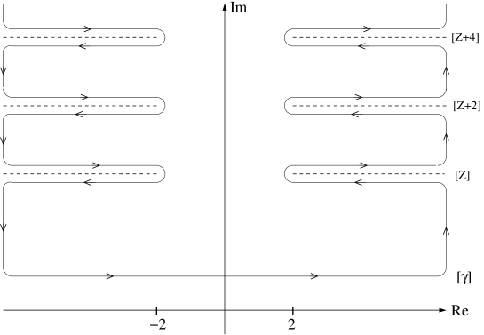
Figure 4: This contour first goes parallel to the real axis and goes around the cuts at $Z+2m$, $Z$ positive integer, $m=0,1,\dots$

According to our basic assumption, $H^{(\alpha)}$ is close to its asymptotic counterpart:

$$H^{(\alpha)}\approx H^{(0)}=\frac{T^{(0)}_{2,3}}{T^{(0)}_{3,2}}=\frac{B_{p}R_{m}}{B_{m}R_{p}}.$$ (103)

$H^{(0)}$ has no zeroes and its poles are at $u_{j}^{\pm}$. Being a smooth deformation, $H^{(\alpha)}$ must also be free of zeroes and must have the same number of poles, which are close to the corresponding asymptotic positions. Let us denote the positions of the poles by $w_{j}^{p(\alpha)}$ and $w_{j}^{m(\alpha)}$, where

$$w_{j}^{p(\alpha)}\approx u_{j}^{+},\qquad\quad w_{j}^{m(\alpha)}\approx u_{j}^{-}.$$ (104)

(These are indeed far from the real axis and all even cuts.)

(102) can now be written as:

$$\begin{split}J^{(\alpha)}(u)=\sum_{j=1}^{N}&\left\{\ln\frac{x(u)-x_{j}^{m(\alpha)}}{\frac{1}{x(u)}-x_{j}^{m(\alpha)}}+\ln\frac{\frac{1}{x(u)}-x_{j}^{p(\alpha)}}{x(u)-x_{j}^{p(\alpha)}}\right\}\\ &+\sum_{Q=1}^{\infty}\int_{-\infty}^{\infty}{\rm d}v\,L_{Q}(v)\left[K^{[Q]}(v,u)-K^{[-Q]}(v,u)\right],\end{split}$$ (105)

where

$$x_{j}^{p(\alpha)}=\frac{1}{x(w_{j}^{p(\alpha)})}\approx x_{j}^{+},\qquad\quad x_{j}^{m(\alpha)}=x(w_{j}^{m(\alpha)})\approx x_{j}^{-}.$$ (106)

5.2 $u_{j}$ related singularities

In the asymptotic solution the singularities of several Y-system elements are given in terms of the set $\{u_{j}\}$, the set of physical rapidities. In the exact solution, the positions of the singular points are smoothly moving away from their asymptotic values and it is possible that positions coinciding in the asymptotic limit move away from each other. However, the Y-system equations give very strong restrictions also for these positions.

In the asymptotic solution the set of real zeroes of $Y^{(\alpha)(0)}_{1|vw}$ coincides with the set of physical rapidities for both values of $\alpha$. After the smooth deformation, the two sets $\{u_{j}^{(\alpha)}\}$, $\alpha=\pm$ may be different, but since $Y^{(\alpha)}_{1|vw}$ are real analytic functions, their zeroes remain real.

Next we use (42) in the $Q=2$ case. This gives that $Y_{2}$ has poles at $u_{j}^{(+)+}$ and $u_{j}^{(-)-}$ or $u_{j}^{(-)+}$ and $u_{j}^{(+)-}$ (for all $j=1,2,\dots N$). Since $Y_{2}$ is real analytic, both options imply that

$$u_{j}^{(+)}=u_{j}^{(-)}=u_{j},\qquad\quad j=1,2,\dots,N.$$ (107)

Now let us use the T-Y relation

$$T_{2,0}^{+}T_{2,0}^{-}=T_{1,0}T_{3,0}(1+Y_{2}).$$ (108)

We conclude that $T_{2,0}$ has poles at $u_{j}^{++}$ and $u_{j}^{--}$. This is very different from the asymptotic solution where $T_{2,0}^{(0)}\equiv 1$. These poles propagate also for higher $T_{a,0}$ functions: (for $a\geq 2$) the first cuts occur at $\pm\frac{i(a+1)}{g}$ but there are poles already at $u_{j}^{[\pm a]}$.

From

$$Y^{(\alpha)}_{1|vw}=\frac{1}{Y_{2,\alpha 1}}=\frac{T_{1,\alpha 1}T_{3,\alpha 1}}{T_{2,\alpha 2}T_{2,0}}$$ (109)

we see that $Y^{(\alpha)}_{1|vw}$ has zeroes at $u_{j}^{++}$ and $u_{j}^{--}$. This is a new feature of the exact solution since $T_{2,0}$ is absent from the denominator of the asymptotic analog of (109).

Using this last piece of information in the Y-system equation (39) we conclude that since the left hand side has double zeroes at $u_{j}^{\pm}$, both $Y_{2}$ and $Y_{+}^{(\alpha)}$ must have poles at $u_{j}^{\pm}$.

Our final conclusion here is that

$${\rm e}^{J^{(\alpha)}}=\frac{Y_{-}^{(\alpha)}}{Y_{+}^{(\alpha)}}$$ (110)

has zeroes at $u_{j}^{\pm}$, hence $w_{j}^{p(\alpha)}=u_{j}^{+}$ and $w_{j}^{m(\alpha)}=u_{j}^{-}$ exactly and we arrive at the final result

$$\frac{Y_{-}^{(\alpha)}}{Y_{+}^{(\alpha)}}=\frac{R_{p}B_{m}}{B_{p}R_{m}}\exp\left\{-\sum_{Q=1}^{\infty}L_{Q}\star K_{Qy}\right\}.$$ (111)

Its logarithmic form is

$$J^{(\alpha)}=j+j_{{\rm red}},$$ (112)

where

$$j=\ln\frac{R_{p}B_{m}}{B_{p}R_{m}}=\sum_{k=1}^{N}\left(\ln\frac{\frac{1}{x}-x_{k}^{+}}{x-x_{k}^{+}}-\ln\frac{\frac{1}{x}-x_{k}^{-}}{x-x_{k}^{-}}\right)$$ (113)

and

$$j_{{\rm red}}=-\sum_{Q=1}^{\infty}L_{Q}\star K_{Qy}.$$ (114)

5.3 Simplifying the equations for $Y_{-}^{(\alpha)}$ and $Y_{+}^{(\alpha)}$

We can now substitute the results (113) and (114) into the TBA equation (52) and write

$$Y_{-}^{(\alpha)}=t^{(\alpha)}_{-}\exp\left\{\ln\left[\frac{1+Y^{(\alpha)}_{1|vw}}{1+Y^{(\alpha)}_{1|w}}\right]\star s-L_{1}\star s+(j^{\epsilon}+j^{\epsilon}_{{\rm red}})\ \check{\star}\ s_{1}\right\}.$$ (115)

We will simplify the $Y^{(\alpha)}_{\pm}$ TBA equations with the help of the following two kernel identities.

$$\begin{split}-2\int\square\,{\rm d}v\,s_{1}(v-u)K_{Qy}(w,v)&+K_{Qy}(w,u)-2\delta_{Q,1}\,s(u-w)=\\ &-K_{Q}(w-u)+2\int_{-\infty}^{\infty}{\rm d}v\,s(u-v)K^{Q1}_{xv}(w,v)\end{split}$$ (116)

and

$$2\int\square\,{\rm d}v\,s_{1}(v-u)j^{\epsilon}(v)=j(u)-\int_{-\infty}^{\infty}{\rm d}v\,s(u-v)\left(\ln\left[\left(\frac{R_{p}^{+}R_{p}^{-}}{R_{m}^{+}R_{m}^{-}}\right)^{2}\frac{Q^{--}}{Q^{++}}\right]\right)(v).$$ (117)

Using the above identities and combining (111) with (115) we get

$$\begin{split}Y^{(\alpha)}_{+}Y^{(\alpha)}_{-}=\left(t_{-}^{(\alpha)}\right)^{2}&\exp\Bigg{\{}2\ln\left[\frac{1+Y^{(\alpha)}_{1|vw}}{1+Y^{(\alpha)}_{1|w}}\right]\star s+\sum_{Q=1}^{\infty}L_{Q}\star\left[-K_{Q}+2K^{Q1}_{xv}\star s\right]\\ &-\ln\left[\left(\frac{R_{p}^{+}R_{p}^{-}}{R_{m}^{+}R_{m}^{-}}\right)^{2}\frac{Q^{--}}{Q^{++}}\right]\star s\Bigg{\}}.\end{split}$$ (118)

6 Dispersion relation for $\Delta$

In this section we determine the $\Delta$ discontinuity using the relations (9) and the corresponding dispersion relation. At the same time we complete the construction of the T-system elements we started in section 4. Our aim is to construct T-system elements that are smooth deformations (similarly to the Y-system elements) of the corresponding asymptotic variables. As we have seen in section 4, this is possible only partially. If, for example, $T_{a,1}$ is close to the corresponding asymptotic $T_{a,1}^{(0)}$ solution for the right hand side of the diagram, then, in general, even for the left-right symmetric ${\mathfrak{sl}(2)}$ cases, $T_{a,-1}$ can be very different from the corresponding asymptotic T-system elements on the left hand side of the diagram. We will work in this gauge which we call the R-gauge and when we want to emphasize this asymmetry we also use the notation $T^{R}_{a,s}$ for $T_{a,s}$. Of course, there also exists an analogous L-gauge, with corresponding T-system elements $T^{L}_{a,s}$, which are close to the asymptotic solution on the left hand side.

We start the calculation by writing

$$Y_{1}=Y_{1,0}=\frac{T_{1,1}T_{1,-1}}{T_{2,0}}=\frac{T^{R}_{1,1}\,T^{R}_{1,-1}}{T_{2,0}}=Y_{d}\,T^{R}_{1,1}\,T^{L}_{1,-1}.$$ (119)

The new object here is

$$Y_{d}=\frac{1}{T_{2,0}}\,\frac{T^{R}_{1,-1}}{T^{L}_{1,-1}}=\frac{t_{1,-1}}{T_{2,0}},$$ (120)

where $t_{a,s}=\frac{T^{R}_{a,s}}{T^{L}_{a,s}}$ is the gauge transformation connecting the two gauges defined above. Corresponding to the three factors in the last expression in (119) we write

$$\Delta=\ln\frac{Y_{1}^{+}}{(Y^{+}_{1})_{*}}=\Delta_{R}+\Delta_{L}+\Delta_{3},$$ (121)

where

$$\Delta_{R}=\ln\frac{(T^{R}_{1,1})^{+}}{((T^{R}_{1,1})^{+})_{*}},\qquad\Delta_{L}=\ln\frac{(T^{L}_{1,-1})^{+}}{((T^{L}_{1,-1})^{+})_{*}},\qquad\Delta_{3}=\ln\frac{Y_{d}^{+}}{(Y_{d}^{+})_{*}}=\ln\frac{t_{1,-1}^{+}}{(t^{+}_{1,-1})_{*}}.$$ (122)

We now rewrite the relation (9), using also the results of the previous section in the form

$$[\Delta]_{\pm 2N}=D^{(\pm 2N)}_{12R}+D^{(\pm 2N)}_{12L}\pm 2(j^{[\epsilon]}+j^{[\epsilon]}_{{\rm red}}),$$ (123)

where

$$D^{(\pm 2N)}_{12R}=\pm\left[\Lambda^{(+)}_{\mp}\right]_{\pm 2N}\pm\sum_{m=1}^{N}\left[\Lambda^{(+)}_{m}\right]_{\pm(2N-m)},\quad D^{(\pm 2N)}_{12L}=\pm\left[\Lambda^{(-)}_{\mp}\right]_{\pm 2N}\pm\sum_{m=1}^{N}\left[\Lambda^{(-)}_{m}\right]_{\pm(2N-m)}$$ (124)

and

$$\Lambda_{\pm}^{(\alpha)}=\ln\left(1-\frac{1}{Y^{(\alpha)}_{\pm}}\right),\qquad\Lambda_{m}^{(\alpha)}=\ln\left(1+\frac{1}{Y^{(\alpha)}_{m|vw}}\right).$$ (125)

So far (except the construction of the T-system elements in section 4) our considerations are valid for any state of the model. From now on, for simplicity, we restrict our attention to states in the ${\mathfrak{sl}(2)}$ (sub-)sector defined in appendix C. We think that our methods can straightforwardly be generalized to generic states, but some of the subsequent formulae are considerably more complicated in the general case. Since the two sides are identical in this special case, in the rest of the paper we can omit the upper index ^(α) of the Y-functions $Y_{\pm}^{(\alpha)}$, $Y_{m|vw}^{(\alpha)}$ or $Y_{m|w}^{(\alpha)}$.

In the ${\mathfrak{sl}(2)}$ (sub-)sector in the asymptotic limit we have

$$Y_{d}^{(0)}=y_{d}\,\qquad\Delta_{3}^{(0)}=\frac{y_{d}^{+}}{(y_{d}^{+})_{*}}=\Delta_{d}$$ (126)

and

$$[\Delta_{3}^{(0)}]_{\pm 2N}=[\Delta_{d}]_{\pm 2N}=\pm 2j^{[\epsilon]},$$ (127)

as discussed in appendix B.

The main part of the calculation is to determine (omitting the upper index $R$ of the T-functions)

$$\Delta_{R}=\ln\frac{T^{+}_{1,1}}{{\cal F}^{+}},$$ (128)

where ${\cal F}^{+}=(T_{1,1}^{+})_{*}$ and similarly we define ${\cal G}^{-}=(T_{1,1}^{-})_{*}$. Note that $\Delta_{R}(u)=p(u)$, the discontinuity which was left undetermined in section 4.

Considerable simplification occurs if we express $D^{(\pm 2N)}_{12R}$ in terms of the T-system elements. For the upper sign we find

$$D^{(2N)}_{12R}=[\ln T^{+}_{1,1}]_{2N}+[\ln T_{N+1,1}]_{N-1}-[\ln T_{N+2,1}]_{N}.$$ (129)

In the gauge we are using $T_{a,1}$ are meromorphic functions in the strip $(-a,a)$, which means that this simplifies to

$$D^{(2N)}_{12R}=[\ln T^{+}_{1,1}]_{2N}.$$ (130)

Next we further specify our gauge: we require that ${\cal F}^{+}$ has no discontinuities in the upper half plane. This is satisfied by the asymptotic function ${\cal F}^{(0)+}$. We then have

$$D^{(2N)}_{12R}=\left[\ln\frac{T^{+}_{1,1}}{{\cal F}^{+}}\right]_{2N}=[\Delta_{R}]_{2N}.$$ (131)

This relation above is in the sense of a discontinuity relation. In this sense one has for any function $f$ and $q$

$$\left[\ln\frac{f}{q}\right]_{Z}=[\ln f]_{Z},$$ (132)

provided $q$ is meromorphic around the cut $Z$. However, as explained in section 2, in the sense of dispersion relation we have for example

$$\int_{2}^{\infty}{\rm d}v[\ln^{\prime}f]_{Z}(v)=\int_{2}^{\infty}{\rm d}v[\ln^{\prime}f(v+\frac{iZ}{g}+i\epsilon)-\ln^{\prime}f(v+\frac{iZ}{g}-i\epsilon)]$$ (133)

and the result will be different if we use $f/q$ instead of $f$ when the meromorphic function $q$ has zeroes/poles on the cut. The correct interpretation of the original relation (9) can be found out from the asymptotic limit of the relation and we find that this subtlety is relevant for the $N=1$ case only and in that relation we have to make the substitution $\Lambda_{1}\Rightarrow\frac{\Lambda_{1}}{p_{2}^{-}}$, where $p_{2}$ is a polynomial whose roots are the real zeroes of $T_{2,1}$. Actually, an equivalent (and simpler) way of taking into account this effect is to simply omit the contribution of these poles from the dispersion relation.

Repeating the same calculation for the lower sign we find

$$D^{(-2N)}_{12R}=-[\ln{\cal G}^{-}+\ln{\cal F}^{+}-\ln T^{+}_{1,1}]_{-2N}-[\ln T_{N+1,1}]_{-(N-1)}+[\ln T_{N+2,1}]_{-N}.$$ (134)

Note that the first term is obtained from

$$1-\frac{1}{Y_{+}}=1-\frac{1}{(Y_{-})_{*}}=1+(Y_{1,1})_{*}=\frac{(T_{1,1}^{+})_{*}\,(T^{-}_{1,1})_{*}}{(T_{2,1})_{*}}=\frac{{\cal F}^{+}\,{\cal G}^{-}}{T_{2,1}}.$$ (135)

Adding to the list of gauge fixing conditions the requirement that ${\cal G}^{-}$ has no discontinuities in the lower half plane (satisfied by the asymptotic ${\cal G}^{(0)-}$) and using the properties of the $T_{a,1}$ functions we have for both signs

$$D^{(\pm 2N)}_{12R}=\left[\ln\frac{T^{+}_{1,1}}{{\cal F}^{+}}\right]_{\pm 2N}=[\Delta_{R}]_{\pm 2N}.$$ (136)

(With the understanding that the correct way of transforming the discontinuity relations into dispersion relations means that we have to omit the contributions of real zeroes in the $N=1$ case.)

At this point we see that the discontinuity relations (9) (rewritten in the form (123)) are satisfied by the asymptotic solution. Indeed, all the properties of the T-functions that we used in the derivation of (136) are equally valid for the asymptotic T-functions and (136), combined with (127) and taking into account the asymptotic relations (15) and the definition of $j$ in (113), prove the statement.

Since in the ${\mathfrak{sl}(2)}$ (sub-)sector the two sides of the problem are identical (in the language of Y-functions) we have

$$[\Delta]_{\pm 2N}=2D^{(\pm 2N)}_{12R}\pm 2(j^{[\epsilon]}+j_{{\rm red}}^{[\epsilon]})$$ (137)

and using (136) this simplifies to

$$[\Delta_{3}]_{\pm 2N}=\pm 2(j^{[\epsilon]}+j_{{\rm red}}^{[\epsilon]}).$$ (138)

We now define $Z_{d}$ and find the relations

$$Y_{d}=y_{d}\,Z_{d},\qquad\Delta_{3}=\Delta_{d}+\Delta_{{\rm red}},\qquad\Delta_{{\rm red}}=\ln\frac{Z_{d}^{+}}{(Z_{d}^{+})_{*}}.$$ (139)

Since asymptotically $Z_{d}^{(0)}=1$, $\Delta_{{\rm red}}^{(0)}=0$ we conclude that in the exact solution ${\rm e}^{\Delta_{{\rm red}}}$ has no zeroes/poles (and has constant asymptotics for large $|u|$). This means that if we define (analogously to $\Gamma^{(\alpha)}(u)$ of section 5)

$$\Gamma_{{\rm red}}(u)=\oint_{\Gamma_{0}}{\rm d}v\,\Delta^{\prime}_{{\rm red}}(v)K(v,u)$$ (140)

and write the corresponding dispersion relation we find

$${\cal D}\Delta_{{\rm red}}=2\sum_{N=1}^{\infty}\,j_{{\rm red}}^{[\epsilon]\prime}\ \check{\star}\ (K^{[2N]}-K^{[-2N]}).$$ (141)

Here the left hand side is the contribution of the narrow strip only (the pole terms vanish) and the right hand side is simply the sum of contributions of the integrals along the even cuts. Using the method explained in section 5 we can “integrate” this relation and get

$$\Delta_{{\rm red}}=2\sum_{N=1}^{\infty}\,j_{{\rm red}}^{[\epsilon]}\ \check{\star}\ (K^{[2N]}-K^{[-2N]}).$$ (142)

6.1 Determination of $\Delta_{R}$

The dispersion relation for $\Delta_{R}$ can be written down using (124) and (136). Proceeding as before we have

$$\begin{split}\Gamma_{R}(u)=\oint_{\Gamma_{0}}{\rm d}v\,\Delta^{\prime}_{R}(v)&K(v,u)=({\cal D}\Delta_{R})(u)+\oint_{[\gamma,2,\infty]}{\rm d}v\,[\ln^{\prime}T_{1,1}^{+}(v)-\ln^{\prime}{\cal F}^{+}(v)]K(v,u)\\ &+\oint_{[-\infty,-2,-\gamma]}{\rm d}v\,[\ln^{\prime}T_{1,1}^{+}(v)-\ln^{\prime}{\cal F}^{+}(v)]K(v,u).\end{split}$$ (143)

The alternative calculation uses the explicit form of $D_{12R}^{(\pm 2N)}$ and its direct integration along the cuts. The contribution of the upper cuts is

$$\begin{split}\Gamma^{{\rm upper}}_{R}(u)&=\sum_{N=1}^{\infty}\,\int\square\,{\rm d}v\,K^{[2N]}(v,u)D^{(2N)\prime}_{12R}(v)\\ =&-\int_{-\infty}^{\infty}{\rm d}v\,K^{[\gamma]}(v,u)\Lambda_{-}^{[\gamma]\prime}(v)+\oint_{[\gamma,2,\infty]}{\rm d}v\,K(v,u)\Lambda_{-}^{\prime}(v)\\ &-\sum_{m=1}^{\infty}\int_{-\infty}^{\infty}{\rm d}v\,K^{[m+\gamma]}(v,u)\Lambda_{m}^{[\gamma]\prime}(v)+\sum_{m=1}^{\infty}\oint_{[\gamma,m,\infty]}{\rm d}v\,K^{[m]}(v,u)\Lambda_{m}^{\prime}(v).\end{split}$$ (144)

Let us consider now the $\Lambda_{m}$ pole terms ($\oint\Lambda^{\prime}_{m}$ terms) separately:

$$\begin{split}&\sum_{m=1}^{\infty}\oint_{[\gamma+1,m+1,\infty]}{\rm d}v\,K^{[m-1]}(v,u)\ln^{\prime}T_{m+1,1}(v)\\ +&\sum_{m=1}^{\infty}\oint_{[\gamma-1,m-1,\infty]}{\rm d}v\,K^{[m+1]}(v,u)\ln^{\prime}T_{m+1,1}(v)\\ -&\sum_{m=0}^{\infty}\oint_{[\gamma,m+1,\infty]}{\rm d}v\,K^{[m+1]}(v,u)\ln^{\prime}T_{m+1,1}(v)\\ -&\sum_{m=2}^{\infty}\oint_{[\gamma,m-1,\infty]}{\rm d}v\,K^{[m-1]}(v,u)\ln^{\prime}T_{m+1,1}(v)\end{split}$$ (145)

We first note that in the integration contours $m-1$ can be changed to $m+1$. This is possible because $T_{m,1}$ has no zeroes/poles/discontinuities on the $m-2$ cut for $m=3,4,\dots$ and $T_{2,1}$ has no poles/discontinuities on the real cut while the contribution of its real zeroes, as we have seen, has to be omitted. We can also change all integrals to have contours of the type $[\gamma,m+1,\infty]$ but here the change of $\gamma\pm 1$ to $\gamma$ requires to add to this sum the corrections

$$-\sum_{m=1}^{\infty}\oint_{[\gamma,\gamma+1]}{\rm d}v\,K^{[m-1]}(v,u)\ln^{\prime}T_{m+1,1}(v)\\ +\sum_{m=1}^{\infty}\oint_{[\gamma-1,\gamma]}{\rm d}v\,K^{[m+1]}(v,u)\ln^{\prime}T_{m+1,1}(v).$$ (146)

The rest of the sum (after taking into account that most terms cancel) simplifies to:

$$\oint_{[\gamma,2,\infty]}{\rm d}v\,K(v,u)\ln^{\prime}T_{2,1}(v)-\oint_{[\gamma,2,\infty]}{\rm d}v\,K(v,u)\ln^{\prime}T_{1,1}^{-}(v)+\oint_{[\gamma-1,\gamma]}{\rm d}v\,K^{+}(v,u)\ln^{\prime}T_{1,1}(v).$$ (147)

Adding also the pole terms corresponding to $\Lambda_{-}$

$$\oint_{[\gamma,2,\infty]}{\rm d}v\,K(v,u)\left[\ln^{\prime}T^{+}_{1,1}(v)+\ln^{\prime}T^{-}_{1,1}(v)-\ln^{\prime}T_{2,1}(v)\right]$$ (148)

the sum of all pole terms becomes:

$$\begin{split}&-\sum_{m=1}^{\infty}\oint_{[\gamma,\gamma+1]}{\rm d}v\,K^{[m-1]}(v,u)\ln^{\prime}T_{m+1,1}(v)\\ &+\sum_{m=0}^{\infty}\oint_{[\gamma-1,\gamma]}{\rm d}v\,K^{[m+1]}(v,u)\ln^{\prime}T_{m+1,1}(v)+\oint_{[\gamma,2,\infty]}{\rm d}v\,K(v,u)\ln^{\prime}T^{+}_{1,1}(v).\end{split}$$ (149)

This can be simplified further using the relation $T_{m,1}=(-1)^{m-1}\tau_{m}\sigma_{m}$ and the facts that $\sigma_{m}$ has no zeroes/poles near the physical strip and $\tau_{1}^{+}$ has no zeroes/poles on the even cuts:

$$\begin{split}-&\sum_{m=2}^{\infty}\oint_{[\gamma,\gamma+1]}{\rm d}v\,K^{[m-2]}(v,u)\ln^{\prime}\tau_{m}(v)+\sum_{m=1}^{\infty}\oint_{[\gamma-1,\gamma]}{\rm d}v\,K^{[m]}(v,u)\ln^{\prime}\tau_{m}(v)\\ +&\int_{-\infty}^{\infty}{\rm d}v\,K^{[\gamma]}(v,u)\ln^{\prime}\tau_{1}^{[1+\gamma]}(v)+\oint_{[\gamma,2,\infty]}{\rm d}v\,K(v,u)\ln^{\prime}\sigma^{+}_{1}(v).\end{split}$$ (150)

It remains to calculate the $\int_{-\infty}^{\infty}$ parts. We write these contributions using the combinations (already used in section 4 for the construction of the T-system elements)

$${\mathscr{L}}_{\pm}=\ln\left[-\tau_{2}\left(1-\frac{1}{Y_{\pm}}\right)\right],\qquad{\mathscr{L}}_{m}=\ln\left[\tau_{m}\tau_{m+2}\left(1+\frac{1}{Y_{m|vw}}\right)\right]$$ (151)

and find

$$\begin{split}-&\int_{-\infty}^{\infty}{\rm d}v\,K^{[\gamma]}(v,u)\Lambda_{-}^{[\gamma]\prime}(v)-\sum_{m=1}^{\infty}\int_{-\infty}^{\infty}{\rm d}v\,K^{[m+\gamma]}(v,u)\Lambda_{m}^{[\gamma]\prime}(v)\\ =-&\int_{-\infty}^{\infty}{\rm d}v\,K^{[\gamma]}(v,u){\mathscr{L}}_{-}^{[\gamma]\prime}(v)-\sum_{m=1}^{\infty}\int_{-\infty}^{\infty}{\rm d}v\,K^{[m+\gamma]}(v,u){\mathscr{L}}_{m}^{[\gamma]\prime}(v)\\ +&\int_{-\infty}^{\infty}{\rm d}v\,K^{[\gamma]}(v,u)\ln^{\prime}\tau_{2}^{[\gamma]}(v)+\sum_{m=1}^{\infty}\int_{-\infty}^{\infty}{\rm d}v\,K^{[m+\gamma]}(v,u)\left[\ln^{\prime}\tau_{m}^{[\gamma]}(v)+\ln^{\prime}\tau_{m+2}^{[\gamma]}(v)\right].\end{split}$$ (152)

Adding everything together and using the identity $\tau_{m}^{+}\tau_{m}^{-}\equiv 1$ in the form $\ln^{\prime}\tau_{m}^{[\gamma-1]}+\ln^{\prime}\tau_{m}^{[\gamma+1]}\equiv 0$ we finally have

$$\begin{split}\Gamma^{{\rm upper}}_{R}(u)&=\oint_{[\gamma,2,\infty]}{\rm d}v\,K(v,u)\ln^{\prime}\sigma_{1}^{+}(v)\\ &-\int_{-\infty}^{\infty}{\rm d}v\,K^{[\epsilon]}(v,u){\mathscr{L}}_{-}^{[\epsilon]\prime}(v)-\sum_{m=1}^{\infty}\int_{-\infty}^{\infty}{\rm d}v\,K^{[m]}(v,u){\mathscr{L}}_{m}^{\prime}(v).\end{split}$$ (153)

Similarly for the contribution of the lower half plane cuts we have

$$\begin{split}\Gamma^{{\rm lower}}_{R}(u)&=\oint_{[-\infty,-2,-\gamma]}{\rm d}v\,K(v,u)\left[\ln^{\prime}\sigma_{1}^{+}(v)-\ln^{\prime}{\cal F}^{+}(v)-\ln^{\prime}{\cal G}^{-}(v)\right]\\ &-\int_{-\infty}^{\infty}{\rm d}v\,K^{[-\epsilon]}(v,u){\mathscr{L}}_{+}^{[-\epsilon]\prime}(v)-\sum_{m=1}^{\infty}\int_{-\infty}^{\infty}{\rm d}v\,K^{[-m]}(v,u){\mathscr{L}}_{m}^{\prime}(v).\end{split}$$ (154)

6.2 The XXX gauge

To calculate $\Delta_{R}$ we need to fix the gauge completely. We will call this complete gauge fixing the XXX gauge and it will not be our final gauge choice yet. Later we will have to perform an additional gauge transformation to arrive at the gauge in which all the T-functions are smooth deformation of the asymptotic solution. This “intermediate” gauge, which will be used in this subsection, we call the XXX gauge because in the $g\rightarrow 0$ limit the system of functions $Y_{m|vw}$, $T_{m,1}$ decouples from the rest and they form the Y-system and T-system of the XXX spin model (the latter in a gauge most natural in that model, namely in which the $T_{m,1}$ functions are polynomials in the spectral parameter $u$).

The XXX gauge is fixed by adding the requirements (in addition to those already imposed in section 4 and this section):

• ${\cal F}_{{\rm XXX}}^{+}$: no zeroes/poles in the upper half plane (no zeroes/poles on the real line) except poles at positions $u_{j}^{+}$ ($j=1,2,\dots,N$).

• ${\cal G}_{{\rm XXX}}^{-}$: no zeroes/poles in the lower half plane.

Recalling that $T_{1,1}^{{\rm XXX}}=\tau_{1}\sigma_{1}$ we can express ${\cal D}\Delta_{R}$ comparing (143) to the sum of (153) and (154). We find

$$\begin{split}{\cal D}&\Delta_{R}(u)=-\int_{-\infty}^{\infty}{\rm d}v\,{\mathscr{L}}_{-}^{[\gamma]\prime}(v)K^{[\gamma]}(v,u)-\int_{-\infty}^{\infty}{\rm d}v\,{\mathscr{L}}_{+}^{[-\epsilon]\prime}(v)K^{[-\epsilon]}(v,u)\\ &-\sum_{m=1}^{\infty}\int_{-\infty}^{\infty}{\rm d}v\,{\mathscr{L}}^{\prime}_{m}(v)k_{m}(v,u)+\oint_{[\gamma,2,\infty]}{\rm d}v\,\left[\ln^{\prime}{\cal F}^{+}(v)-\ln^{\prime}\tau_{1}^{+}(v)\right]K(v,u)\\ &\qquad\qquad+\oint_{[-\infty,-2,-\gamma]}{\rm d}v\,K(v,u)[-\ln^{\prime}\tau_{1}^{+}(v)].\end{split}$$ (155)

We can calculate the pole terms ($\oint$ terms) of this expression using the residue theorem:

$$-2\pi i\sum_{j=1}^{N}K(u_{j}^{+},u)+2\pi i\sum_{j=1}^{N}\sum_{\nu=-\infty}^{\infty}\left\{K(u_{j}^{+}+\frac{4\nu i}{g},u)-K(u_{j}^{-}+\frac{4\nu i}{g},u)\right\}.$$ (156)

Their contribution, after “integration”, as explained in section 5, becomes

$${\cal W}(u)=\sum_{j=1}^{N}\sigma(u,u_{j}^{+})+\sum_{j=1}^{N}\sum_{\nu=-\infty}^{\infty}\left\{\sigma(u,u_{j}^{-}+\frac{4\nu i}{g})-\sigma(u,,u_{j}^{+}+\frac{4\nu i}{g})\right\}.$$ (157)

Note that using the definition

$$\vartheta_{1}^{+}(u)=\prod_{j=1}^{N}\prod_{\nu=-\infty}^{\infty}\frac{S(u,u_{j}^{-}+\frac{4\nu i}{g})}{S(u,u_{j}^{+}+\frac{4\nu i}{g})},$$ (158)

where the notation indicates that this function has exactly the same zeroes/poles as $\tau_{1}^{+}$, we have

$${\rm e}^{{\cal W}(u)}=\vartheta_{1}^{+}(u)\prod_{j=1}^{N}S(u,u_{j}^{+}).$$ (159)

We can now write the “integrated” version of (155):

$$\begin{split}\Delta_{R}(u)=-\int_{-\infty}^{\infty}{\rm d}v\,&{\mathscr{L}}_{-}^{[\gamma]}(v)K^{[\gamma]}(v,u)-\int_{-\infty}^{\infty}{\rm d}v\,{\mathscr{L}}_{+}^{[-\epsilon]}(v)K^{[-\epsilon]}(v,u)\\ -&\sum_{m=1}^{\infty}\int_{-\infty}^{\infty}{\rm d}v\,{\mathscr{L}}_{m}(v)k_{m}(v,u)+{\cal W}(u)-\ln x^{2}(u).\end{split}$$ (160)

Note that this formula is valid just above the real line in the strip $0<{\rm Im}u<\frac{\gamma}{g}$.

The last term in (160) is necessary to balance the large $|u|$ asymptotics of the equation. We know that in this limit (just above the real line)

$${\mathscr{L}}_{+}(u),\,{\mathscr{L}}_{-}(u)\approx-\ln|u|,\qquad\Delta_{R}(u)\approx\ln|u|$$ (161)

and we see that (160) is asymptotically correct because if a function $f$ behaves asymptotically as $f(u)\approx\ln|u|$ then convolution with the kernel $K^{[\alpha]}$ gives

$$f\star K^{[\alpha]}\approx-\frac{1}{2}\ln|u|.$$ (162)

Finally by manipulating the integrals containing ${\mathscr{L}}_{+},\,{\mathscr{L}}_{-}$ we write our final result for the discontinuity $\Delta_{R}$:

$$\begin{split}\Delta_{R}(u)={\mathscr{L}}_{-}(u)-&\int_{-2}^{2}{\rm d}v\,[{\mathscr{L}}_{-}(v)+{\mathscr{L}}_{+}(v)]K(v,u)\\ -&\sum_{m=1}^{\infty}\int_{-\infty}^{\infty}{\rm d}v\,{\mathscr{L}}_{m}(v)k_{m}(v,u)+{\cal W}(u)-\ln x^{2}(u).\end{split}$$ (163)

Note that the last term is chosen here so that $\Delta_{R}(\pm 2)=0$ is satisfied. The price we have to pay is that this term creates a cut along the imaginary axis (but neither $\Delta^{\prime}_{R}(u)$ nor ${\rm e}^{\Delta_{R}(u)}$ have discontinuities there).

Our final result for the discontinuity $\Delta(u)$ in the ${\mathfrak{sl}(2)}$ (sub-)sector is

$$\begin{split}&\qquad\qquad\Delta=2\Delta_{R}+\Delta_{d}+\Delta_{{\rm red}}\\ &=2{\mathscr{L}}_{-}-2({\mathscr{L}}_{-}+{\mathscr{L}}_{+})\ \hat{\star}\ K-2\sum_{m=1}^{\infty}{\mathscr{L}}_{m}\star k_{m}+2{\cal W}-L\ln x^{2}+\ln\frac{{\cal D}_{1}^{+}}{({\cal D}_{1}^{+})_{*}}+\Delta_{{\rm red}}.\end{split}$$ (164)

Here we have used (351) to write

$$\Delta_{d}=-J\ln x^{2}+\ln\frac{{\cal D}_{1}^{+}}{({\cal D}_{1}^{+})_{*}}.$$ (165)

We note that the renormalization $J\rightarrow L=J+2$ is due to the addition of the zero mode contribution in (160) and it is universal (we see this here for the case of states in the ${\mathfrak{sl}(2)}$ (sub-)sector). Indeed, this universality was shown for generic states in [36]. The physical meaning of $L$ is that it is the maximal value of the $J$-charge within the $psu(2,2|4)$ supermultiplet to which the given state belongs.

The result (164), together with $J^{(\alpha)}$ calculated in section 5, completes the set of TBA integral equations of section 3 for the excited states in this sector of the model. This system of integral equations is now closed. It still has to be supplemented by the quantization conditions for the discrete parameters appearing in the source terms. This will be discussed in section 9.

At this point we would like to emphasize that the Y-system and discontinuity relations (with some additional qualitative information on local singularities) determine the set of TBA equations completely. We can summarize the logic of calculating the full $\Delta$ (including the dressing phase part $\Delta_{d}$) as follows. First we fix a gauge such that the T-factors in (119) satisfy (136) and thus the discontinuity relations simplify to (138). Next we take (139) as an Ansatz and use the (nontrivial) computations presented in appendix B to show that (138) is now further reduced to

$$[\Delta_{red}]_{\pm 2N}=\pm 2j_{red}^{[\epsilon]},$$ (166)

which can be solved easily using (140-142). Of course, by writing (139) we actually use the known formulae for the dressing phase part and verify it satisfies the relations (320-321). This simplifies our job here. However, even if we had not known the solution for $\Delta_{d}$ given by (165) we could have calculated it from the discontinuity relation (320) by transforming it into a dispersion relation as we did for the other building blocks.

In this section we obtained the result (163) by a long direct calculation. An alternative logic could have been to simply postulate the result (163) for $p(u)=\Delta_{R}(u)$ and show that the requirements on the upper/lower half plane behavior of the ${\cal F}^{+}$/${\cal G}^{-}$ functions, which we used in the calculation, are indeed satisfied.

To show this, we start from

$$T^{{\rm XXX}}_{1,1}=\tau_{1}\sigma_{1},\qquad\quad\sigma_{1}=\frac{q^{+}}{q^{-}}\sigma_{1}^{(0)},$$ (167)

where

$$\sigma_{1}^{(0)}=\exp\left\{{\mathscr{L}}_{-}^{[\epsilon]}\star(\kappa^{-}-\kappa^{+})+\sum_{m=1}^{\infty}{\mathscr{L}}_{m}\star(\kappa^{[-m-1]}-\kappa^{[m+1]})\right\}$$ (168)

and $q$ is defined in (75). Here we introduced the notation

$$\kappa(v,u)=\frac{1}{2\pi i}\,\frac{1}{v-u},\qquad\qquad K_{a}=\kappa^{[-a]}-\kappa^{[a]}.$$ (169)

Note that $K(v,u)-\kappa(v,u)$ is regular at $v=u$.

The discontinuity relation is

$$\frac{q(u+i\epsilon)}{q(u-i\epsilon)}={\rm e}^{-p(u+i\epsilon)},\qquad|u|\geq 2$$ (170)

and just above the real line, in the strip $0<{\rm Im}u<\frac{\gamma}{g}$ we have

$$p={\mathscr{L}}_{-}-({\mathscr{L}}_{-}+{\mathscr{L}}_{+})\ \hat{\star}\ K-\sum_{m=1}^{\infty}{\mathscr{L}}_{m}\star k_{m}+{\cal W}-\ln x^{2}$$ (171)

and

$$\sigma_{1}^{(0)+}=\exp\left\{{\mathscr{L}}_{-}+{\mathscr{L}}_{-}^{[\epsilon]}\star(\kappa^{--}-\kappa)+\sum_{m=1}^{\infty}{\mathscr{L}}_{m}\star(\kappa^{[-m-2]}-\kappa^{[m]})\right\}$$ (172)

and finally

$$\begin{split}{\cal F}^{+}_{{\rm XXX}}&=\left(T_{1,1}^{{\rm XXX}}\right)^{+}{\rm e}^{-p}=x^{2}\frac{q^{++}}{q}\,\frac{\tau_{1}^{+}}{{\rm e}^{\cal W}}\,\exp\Big{\{}({\mathscr{L}}_{-}+{\mathscr{L}}_{+})\ \hat{\star}\ K\\ +&{\mathscr{L}}_{-}^{[\epsilon]}\star(\kappa^{--}-\kappa)+\sum_{m=1}^{\infty}{\mathscr{L}}_{m}\star(K^{[m]}-\kappa^{[m]}+K^{[-m]}+\kappa^{[-m-2]})\Big{\}}.\end{split}$$ (173)

From this result we see that there are indeed no zeroes/poles/discontinuities in the upper half plane, except for the poles at the positions $u_{j}^{+}$.

Similarly, just below the real line, in the strip $-\frac{\gamma}{g}<{\rm Im}u<0$ we have

$$\sigma_{1}^{(0)-}=\exp\left\{{\mathscr{L}}_{-}+{\mathscr{L}}_{-}^{[\epsilon]}\star(\kappa-\kappa^{++})+\sum_{m=1}^{\infty}{\mathscr{L}}_{m}\star(\kappa^{[-m]}-\kappa^{[m+2]})\right\},$$ (174)

$$p=-{\mathscr{L}}_{+}-({\mathscr{L}}_{-}+{\mathscr{L}}_{+})\ \hat{\star}\ K-\sum_{m=1}^{\infty}{\mathscr{L}}_{m}\star k_{m}+{\cal W}-\ln x^{2},$$ (175)

and noting that from (11) we have $I={\mathscr{L}}_{-}-{\mathscr{L}}_{+}$

$$m=I-p={\mathscr{L}}_{-}+({\mathscr{L}}_{-}+{\mathscr{L}}_{+})\ \hat{\star}\ K+\sum_{m=1}^{\infty}{\mathscr{L}}_{m}\star k_{m}-{\cal W}+\ln x^{2},$$ (176)

and finally

$$\begin{split}{\cal G}^{-}_{{\rm XXX}}&=\left(T_{1,1}^{{\rm XXX}}\right)^{-}{\rm e}^{-m}=\frac{1}{x^{2}}\,\frac{q}{q^{--}}\,\frac{{\rm e}^{\cal W}}{\tau_{1}^{+}}\,\exp\Big{\{}-({\mathscr{L}}_{-}+{\mathscr{L}}_{+})\ \hat{\star}\ K\\ +&{\mathscr{L}}_{-}^{[\epsilon]}\star(\kappa-\kappa^{++})+\sum_{m=1}^{\infty}{\mathscr{L}}_{m}\star(\kappa^{[-m]}-K^{[-m]}-K^{[m]}-\kappa^{[m+2]})\Big{\}}.\end{split}$$ (177)

We see that there are indeed no zeroes/poles/discontinuities in this expression in the lower half plane.

6.3 Complete gauge fixing

It is possible to show that the XXX gauge we have been using in this section is a complete gauge fixing. This means that given an exact solution of the Y-system equations, which also satisfies the reality conditions and the relation between $Y_{-}$ and $Y_{+}$ and has the cut structure described in section 2, we can always construct the corresponding XXX gauge T-system elements $T^{{\rm XXX}}_{a,s}$, which satisfy all the requirements listed below and this construction is unique.

The requirements are

• $T^{{\rm XXX}}_{0,s}\equiv 1$.

• $T^{{\rm XXX}}_{a,0}$ are given as constructed explicitly in section 4 using the chain lemma.

• $T^{{\rm XXX}}_{a,1}$ have discontinuities along the cuts $\pm(a+2m)$, $m=0,1,\dots$

• The roots of $T^{{\rm XXX}}_{a,1}$ in the physical strip are the same as those of $\tau_{a}$ and there are no poles in this strip.

• ${\cal F}_{{\rm XXX}}^{+}$: no zeroes/poles/discontinuities in the upper half plane (no zeroes/poles on the real line) except poles at positions $u_{j}^{+}$ ($j=1,2,\dots,N$).

• ${\cal G}_{{\rm XXX}}^{-}$: no zeroes/poles/discontinuities in the lower half plane.

• The large $|u|$ behavior is the same as for the asymptotic solution.

We now perform the final gauge transformation which brings the T-system solution in a gauge (we will call it the BA gauge) where the T-system functions $T_{a,s}$ for $s\geq 0$ are close to the asymptotic (Bethe Ansatz) solution $T_{a,s}^{(0)}$. This is achieved by defining

$$T_{1,1}=\beta\,T^{{\rm XXX}}_{1,1},\qquad\quad\beta=\frac{Q^{--}}{Q}.$$ (178)

We see that $T_{1,1}$ has no zeroes/poles in the physical strip. From

$${\cal F}^{+}=\frac{Q^{-}}{Q^{+}}\,{\cal F}^{+}_{{\rm XXX}},\qquad\quad{\cal G}^{-}=\frac{Q^{[-3]}}{Q^{-}}\,{\cal G}^{-}_{{\rm XXX}}$$ (179)

we see that ${\cal F}^{+}$/${\cal G}^{-}$ has no zeroes/poles/discontinuities in the upper/lower half plane.

From the list of requirements above and the modification induced by (178) we see that the BA gauge T-functions are indeed smooth deformations of the asymptotic solution, satisfying the same requirements. Note that the final results for $p=\Delta_{R}$ and the full $\Delta$ are unchanged since the transformation (178) is meromorphic.

7 Simplified $Y_{1}$ equation

In this section we want to simplify the TBA equation (51) in order to be able to compare it with the results of [34]. First we simplify $\Delta_{R}$ and $\Delta_{{\rm red}}$ and use these results in the $Y_{1}$ TBA equation (51).

7.1 Simplifying $\Delta_{R}$

Let us introduce the new TBA variables $W_{a}$ with the definitions

$$Y_{a}=\tau_{a}^{2}\,W_{a},\qquad a=2,3,\dots,\qquad Y_{1}=W_{1}.$$ (180)

$W_{a}$ ($a=1,2,\dots$) have no zeroes/poles in the physical strip. In terms of these variables we rewrite (50) in the form

$$\ln W_{a} = \left\{2{\mathscr{L}}_{a-1}+\ln W_{a+1}+\ln W_{a-1}-L_{a+1}-L_{a-1}\right\}\star s,\qquad a=3,4,\dots$$ (181)

$$\ln W_{2} = \left\{2{\mathscr{L}}_{1}+\ln W_{3}+\ln W_{1}-L_{3}-L_{1}-\ln\tau_{1}^{2}\right\}\star s.$$ (182)

The simplification of (163) is based on the kernel identity [26]

$$k_{a}+\delta_{a,1}\,s=s\star(k_{a+1}+k_{a-1}),\qquad a=1,2,\dots$$ (183)

where $k_{0}(w,v)=2\Theta(4-w^{2})K(w,v)$. The convolution of (181) with $(k_{a}+k_{a-2})$ (from the right) gives for $a=3,4\dots$, after using (183)

$$\ln W_{a}*(k_{a}+k_{a-2})=(2{\mathscr{L}}_{a-1}+\ln W_{a+1}+\ln W_{a-1}-L_{a+1}-L_{a-1})\star k_{a-1}$$ (184)

and from (182) we get

$$\ln W_{2}*(k_{2}+k_{0})=\ln W_{2}+(2{\mathscr{L}}_{1}+\ln W_{3}+\ln W_{1}-L_{3}-L_{1})\star k_{1}-\ln\tau_{1}^{2}\star k_{1}.$$ (185)

Using the methods we employed in section 6 for the calculation of pole terms we can evaluate the convolution $\ln\tau_{1}^{2}\star k_{1}$:

$$\ln\tau_{1}^{2}\star k_{1}=2{\cal W}-{\cal W}_{0},\qquad{\cal W}_{0}(u)=\sum_{j=1}^{N}[\sigma(u,u_{j}^{+})+\sigma(u,u_{j}^{-})].$$ (186)

The equations (184) and (185) can be used to express the terms containing ${\mathscr{L}}_{m}$ in (163). Many terms cancel and we find

$$\begin{split}2\sum_{m=1}^{\infty}{\mathscr{L}}_{m}\star k_{m}=\sum_{Q=1}^{\infty}(L_{Q}&+L_{Q+2})\star k_{Q}-\ln W_{2}\\ &+2\ln W_{2}\ \hat{\star}\ K-\ln Y_{1}\star k_{1}+2{\cal W}-{\cal W}_{0}.\end{split}$$ (187)

This can be used to write the simplified $\Delta_{R}$ formula

$$\begin{split}2\Delta_{R}&=-\sum_{Q=1}^{\infty}(L_{Q}+L_{Q+2})\star k_{Q}+\ln\left\{Y_{2}\left(1-\frac{1}{Y_{-}}\right)^{2}\right\}\\ &-2\ln\left\{Y_{2}\left(1-\frac{1}{Y_{-}}\right)\left(1-\frac{1}{Y_{+}}\right)\right\}\ \hat{\star}\ K+{\cal W}_{0}-2\ln x^{2}+\ln Y_{1}\star k_{1}.\end{split}$$ (188)

7.2 Simplifying $\Delta_{{\rm red}}$

We start from

$$\Delta_{{\rm red}}(u) = 2\sum_{N=1}^{\infty}\int\square\,{\rm d}v\,j_{{\rm red}}(v+i\epsilon)\left\{K^{[2N]}(v,u)-K^{[-2N]}(v,u)\right\}$$ (189)

$$= \sum_{Q=1}^{\infty}\int_{-\infty}^{\infty}{\rm d}w\,L_{Q}(w)\Sigma_{Q}(w,u),$$ (190)

where

$$\Sigma_{Q}(w,u)=2\sum_{N=1}^{\infty}\int\square\,{\rm d}v\,\left\{K^{[Q]}(w,v+i\epsilon)-K^{[-Q]}(w,v+i\epsilon)\right\}\left\{K^{[2N]}(v,u)-K^{[-2N]}(v,u)\right\}.$$ (191)

The kernel identity we need here is

$$\int\square\,{\rm d}v\,K^{[\pm 2N]}(v,u)K_{Qy}(w,v+i\epsilon)=\pm K^{[\pm(2N+Q)]}(w,u)\mp\int_{-2}^{2}{\rm d}v\,K_{Qy}(w,v)K^{[\pm 2N]}(v,u).$$ (192)

Using it we find

$$\begin{split}\Sigma_{Q}(w,u)&=2\sum_{N=1}^{\infty}\left\{\int_{-2}^{2}{\rm d}v\,K_{Qy}(w,v)k_{2N}(v,u)-k_{2N+Q}(w,u)\right\}\\ &=2I_{Q}(w,u)-2\int_{-2}^{2}{\rm d}v\,K_{Qy}(w,v)I_{0}(v,u)=2\check{K}^{\Sigma}_{Q}(w,u).\end{split}$$ (193)

7.3 The $Y_{1}$ equation

The results of the previous two subsections can be used to simplify the full discontinuity $\Delta$. We get (with $L=J+2$)

$$\Delta=\ln\frac{{\cal D}_{1}^{+}}{({\cal D}_{1}^{+})_{*}}+\Delta^{(L)}+\Delta^{(12)}+{\cal W}_{0}+\ln\left\{Y_{2}\left(1-\frac{1}{Y_{-}}\right)^{2}\right\}-L\ln x^{2},$$ (194)

where

$$\Delta^{(L)}=\sum_{Q=1}^{\infty}L_{Q}\star(2\check{K}^{\Sigma}_{Q}-k_{Q})-\sum_{Q=3}^{\infty}L_{Q}\star k_{Q-2}$$ (195)

and

$$\Delta^{(12)}=\ln Y_{1}\star k_{1}-2\ln\left\{Y_{2}\left(1-\frac{1}{Y_{-}}\right)\left(1-\frac{1}{Y_{+}}\right)\right\}\ \hat{\star}\ K.$$ (196)

The simplified TBA equation for $Y_{1}$ becomes

$$\ln Y_{1} = \ln\left\{Y_{2}\left(1-\frac{1}{Y_{-}}\right)^{2}\right\}\star s-L_{2}\star s-\Delta\ \check{\star}\ s$$ (197)

$$= \ln\left\{Y_{2}\left(1-\frac{1}{Y_{-}}\right)^{2}\right\}\ \hat{\star}\ s-L_{2}\star s-\Delta_{{\rm eff}}\ \check{\star}\ s,$$ (198)

where

$$\Delta_{{\rm eff}}=\Delta^{(L)}+\Delta^{(12)}+\Delta^{({\rm source})}-L\ln x^{2}$$ (199)

and

$$\Delta^{({\rm source})}={\cal W}_{0}+\ln\frac{{\cal D}_{1}^{+}}{({\cal D}_{1}^{+})_{*}}.$$ (200)

Using the results of appendix B we can write

$$\frac{{\cal D}_{1}^{+}}{({\cal D}_{1}^{+})_{*}}=\left(\frac{B_{p}}{R_{p}}\right)^{2}\exp\left\{2\sum_{j=1}^{N}[G(u,x_{j}^{+})-G(u,x_{j}^{-})]\right\},$$ (201)

where

$$iG(u,\xi)=\Phi\left(\frac{1}{x(u)},\xi\right)-\Phi(x(u),\xi)+\psi(u,\xi)$$ (202)

and the source term simplifies to

$$\Delta^{({\rm source})}=\ln\left(\frac{B_{m}B_{p}}{R_{m}R_{p}}\right)+2\sum_{j=1}^{N}\left\{G(u,x_{j}^{+})-G(u,x_{j}^{-})\right\}.$$ (203)

If we use for $G(u,\xi)$ the alternative representation

$$G(u,\xi)=\int_{-2}^{2}{\rm d}v\,\ln\left(\frac{\frac{1}{x(v)}-\xi}{x(v)-\xi}\right)\,I_{0}(v,u)$$ (204)

we can check that our simplified equation (198) agrees with eq. (4.10) of ref. [34].

8 Canonical (and hybrid) equations for $Y_{Q}$

Using the $W_{a}$ variables introduced in section 7 we can rewrite the Y-system equations (42-43) in the form

$$\frac{W_{a}^{+}W_{a}^{-}}{W_{a+1}W_{a-1}}=\xi_{a},\qquad a=1,2,\dots,\qquad W_{0}\equiv 1,$$ (205)

where

$$\ln\xi_{a} = 2{\mathscr{L}}_{a-1}-L_{a+1}-L_{a-1}-\delta_{a,2}\ln\tau_{1}^{2}\,\qquad a=2,3,\dots,$$ (206)

$$\ln\xi_{1} = 2{\mathscr{L}}_{-}-L_{2}.$$ (207)

Using the chain lemma of section 4 we can transform (205) into the integral equations

$$\ln W_{a}=\sum_{A=1}^{\infty}\ln\xi_{A}\star\ell^{A}_{a}-\Delta\ \check{\star}\ K_{a}.$$ (208)

Here $\Delta$ is given by (164).

8.1 Kernel identities

We now list a number of kernel identities that are needed to simplify the integral equations (208).

We start by writing the kernel defined by (291) as

$$\begin{split}K^{QM}_{vwx}(u,v)&=\frac{1}{2}K_{Q+M}(u-v)-\frac{1}{2}K_{Q-M}(u-v)+\sum_{j=1}^{Q-1}K_{M-Q+2j}(u-v)\\ &+\frac{1}{2}k_{Q}(u,v^{[M]})-\frac{1}{2}k_{Q}(u,v^{[-M]}).\end{split}$$ (209)

Next we write the identity

$$K(y,v)K_{a}(v-u)=K(y,u^{[a]})K(v,u^{[a]})-K(y,u^{[-a]})K(v,u^{[-a]})-K_{a}(y-u)K(v,y)$$ (210)

and integrate with respect to $v$ just above the cuts using the result

$$\int\square{\rm d}v\,K(v+i\epsilon,\alpha)=\frac{1}{2}$$ (211)

and obtain

$$K\ \check{\star}\ K_{a}=\frac{1}{2}K_{ya}-\frac{1}{2}K_{a}.$$ (212)

This can be used to get the further identities

$$K^{Aa}_{vwx}=\ell^{A+1}_{a}+k_{A}\ \check{\star}\ K_{a}$$ (213)

and for the “fermionic” kernels defined by (286)

$$K^{ya}_{-} = \frac{1}{2}K_{ya}+\frac{1}{2}K_{a}=K_{a}+K\ \check{\star}\ K_{a},$$ (214)

$$K^{ya}_{+} = \frac{1}{2}K_{ya}-\frac{1}{2}K_{a}=K\ \check{\star}\ K_{a}.$$ (215)

The most important identity is

$$K^{\Sigma}_{QQ^{\prime}}=\check{K}^{\Sigma}_{Q}\ \check{\star}\ K_{Q^{\prime}},$$ (216)

which is proven in [26]. Using also

$$\ell^{Q+1}_{a}+\ell^{Q-1}_{a}=K_{Qa}$$ (217)

we can write

$$\ell^{Q+1}_{a}+\ell^{Q-1}_{a}+\Sigma_{Q}\ \check{\star}\ K_{a}=K_{Qa}+2\check{K}^{\Sigma}_{Q}\ \check{\star}\ K_{a}=K_{Qa}+2K^{\Sigma}_{Qa}=-K^{Qa}_{{\mathfrak{sl}(2)}}.$$ (218)

Finally we write the chain lemma for $b_{a}=\frac{x^{[a]}}{x^{[-a]}}$. Since it satisfies $b_{a}^{+}b_{a}^{-}=b_{a+1}b_{a-1}$ in this case $\xi_{a}\equiv 1$ and the only nontrivial object is

$$p=\ln\frac{b_{1}^{+}}{(b_{1}^{+})_{*}}=-\ln x^{2}$$ (219)

and we find from the chain lemma

$$\tilde{\cal E}_{a}=-\ln b_{a}=-\ln x^{2}\ \check{\star}\ K_{a}.$$ (220)

8.2 Canonical TBA equations

Collecting all the terms proportional to ${\mathscr{L}}_{m}$, ${\mathscr{L}}_{\pm}$ or $L_{Q}$ and using the above identities and the simplifications of subsection 7.2 we can rewrite (208). This can be called the canonical $W_{a}$ TBA equation and is of the form

$$\ln W_{a}=-L\tilde{\cal E}_{a}+f_{a}+2\sum_{m=1}^{\infty}{\mathscr{L}}_{m}\star K^{ma}_{vwx}+2{\mathscr{L}}_{-}\ \hat{\star}\ K^{ya}_{-}+2{\mathscr{L}}_{+}\ \hat{\star}\ K^{ya}_{+}+\sum_{Q=1}^{\infty}L_{Q}\star K^{Qa}_{{\mathfrak{sl}(2)}}.$$ (221)

Here an alternative form of the ${\mathscr{L}}_{\pm}$ terms is

$$2{\mathscr{L}}_{-}\ \hat{\star}\ K^{ya}_{-}+2{\mathscr{L}}_{+}\ \hat{\star}\ K^{ya}_{+}=\ln\left(\frac{1-\frac{1}{Y_{-}}}{1-\frac{1}{Y_{+}}}\right)\ \hat{\star}\ K_{a}+\ln\left(\tau_{2}^{2}\left(1-\frac{1}{Y_{-}}\right)\left(1-\frac{1}{Y_{+}}\right)\right)\ \hat{\star}\ K_{ya}$$ (222)

and the source term $f_{a}$ can be written as

$$f_{a}=-\ln\tau_{1}^{2}\star(K_{a+1}+K_{a-1})-\left(2{\cal W}+\ln\frac{{\cal D}_{1}^{+}}{({\cal D}_{1}^{+})_{*}}\right)\ \check{\star}\ K_{a}.$$ (223)

The source term can be simplified using the chain lemma for

$${\cal D}_{a}(u)=\prod_{j=1}^{N}S^{a1*}_{{\mathfrak{sl}(2)}}(u,u_{j})=\prod_{j=1}^{N}\left\{S^{1*a}_{{\mathfrak{sl}(2)}}(u_{j},u)\right\}^{-1}.$$ (224)

${\cal D}_{a}$ satisfy

$${\cal D}_{a}^{+}{\cal D}_{a}^{-}={\cal D}_{a+1}{\cal D}_{a-1},\qquad a=1,2,\dots,\qquad{\cal D}_{0}\equiv 1.$$ (225)

However, ${\cal D}_{2}$ has poles at $u_{j}^{+}$ and zeroes at $u_{j}^{-}$, so the chain lemma does not directly apply for the ${\cal D}_{a}$ functions. This problem is solved by introducing

$$d_{a}(u)=\frac{Q^{[a+1]}(u)Q^{[a-1]}(u)}{Q^{[-a-1]}(u)Q^{[1-a]}(u)}=\prod_{j=1}^{N}\frac{1}{S_{a+1}(u-u_{j})S_{a-1}(u-u_{j})}$$ (226)

and noting that $\tilde{\cal D}_{a}=\frac{{\cal D}_{a}}{d_{a}}$ also satisfy the chain lemma equations with $\xi_{a}\equiv 1$ and do not have any singularities near the physical strip and thus can be represented as

$$\tilde{\cal D}_{a}=\exp\left\{-\ln\frac{{\cal D}_{1}^{+}}{({\cal D}_{1}^{+})_{*}}\ \check{\star}\ K_{a}\right\}.$$ (227)

Using this representation the source term becomes

$$\begin{split}f_{a}(u)=&-\sum_{j=1}^{N}\ln S^{1*a}_{{\mathfrak{sl}(2)}}(u_{j},u)-\left[\ln\tau_{1}^{2}\star(K_{a+1}+K_{a-1})\right](u)\\ &+\sum_{j=1}^{N}\left[\ln S_{a+1}(u-u_{j})+\ln S_{a-1}(u-u_{j})\right]-2\left[T^{\epsilon}\star k_{1}\ \check{\star}\ K_{a}\right](u).\end{split}$$ (228)

Here we used the result

$${\cal W}=T^{\epsilon}\star k_{1},$$ (229)

which can be proved by using the residue theorem. We have defined

$$T^{\pm\epsilon}(u)=\sum_{j=1}^{N}\ln t(u-u_{j}\pm i\epsilon).$$ (230)

It is easy to prove that

$$\left[(T^{\epsilon}-T^{-\epsilon})\star\ell^{2}_{a}\right](u) = -\sum_{j=1}^{N}\left[\ln S_{a+1}(u-u_{j})+\ln S_{a-1}(u-u_{j})\right],$$ (231)

$$(T^{\epsilon}+T^{-\epsilon})\star\ell^{2}_{a} = \ln\tau_{1}^{2}\star\ell^{2}_{a}$$ (232)

and with the help of these relations and the results in the previous subsection we can write the final form of the source terms:

$$f_{a}(u) = -\sum_{j=1}^{N}\ln S^{1*a}_{{\mathfrak{sl}(2)}}(u_{j},u)-2\left[T^{\epsilon}\star(\ell^{2}_{a}+k_{1}\ \check{\star}\ K_{a})\right](u)$$ (233)

$$= -\sum_{j=1}^{N}\ln S^{1*a}_{{\mathfrak{sl}(2)}}(u_{j},u)-2\left[T^{\epsilon}\star K^{1a}_{vwx}\right](u).$$ (234)

8.3 Hybrid TBA equations

We can get rid of the infinite sums containing the functions ${\mathscr{L}}_{m}$ by the following trick [34]. We write the (46) TBA equation as

$$r_{m}-{\mathscr{L}}_{m}=(r_{m+1}+r_{m-1}-L_{m+1})\star s+\delta_{m,1}\ln\left[\frac{1-Y_{-}}{1-Y_{+}}\right]\ \hat{\star}\ s,\qquad m=1,2,\dots,$$ (235)

where we introduced the notation $r_{m}=\ln[1+Y_{m|vw}],\ m=1,2,\dots,r_{0}\equiv 0$. We now assume that the kernel functions ${\mathscr{K}}_{m}$ satisfy the relations

$${\mathscr{K}}_{m}-s\star({\mathscr{K}}_{m+1}+{\mathscr{K}}_{m-1})=j_{m},\qquad m=1,2,\dots,\qquad{\mathscr{K}}_{0}\equiv 0$$ (236)

with some $j_{m}$. We take the convolution of (235) with ${\mathscr{K}}_{m}$ and sum over $m$. We find

$$\sum_{m=1}^{\infty}{\mathscr{L}}_{m}\star{\mathscr{K}}_{m}=\sum_{m=1}^{\infty}L_{m}\star s\star{\mathscr{K}}_{m-1}+\sum_{m=1}^{\infty}r_{m}\star j_{m}-\ln\left[\frac{1-Y_{-}}{1-Y_{+}}\right]\ \hat{\star}\ s\star{\mathscr{K}}_{1}.$$ (237)

We now choose ${\mathscr{K}}_{m}=K^{ma}_{vwx}$. In this case

$$j_{m}=\delta_{m+1,a}s+\delta_{m,1}s\ \hat{\star}\ K_{ya}$$ (238)

and using the above trick the TBA equations can be brought to the form

$$\begin{split}\ln W_{a}=&-L\tilde{\cal E}_{a}+f_{a}+2r_{a-1}\star s+2r_{1}\star s\ \hat{\star}\ K_{ya}\\ &-2\ln\left[\frac{1-Y_{-}}{1-Y_{+}}\right]\ \hat{\star}\ s\star K^{1a}_{vwx}+2{\mathscr{L}}_{-}\ \hat{\star}\ K^{ya}_{-}+2{\mathscr{L}}_{+}\ \hat{\star}\ K^{ya}_{+}\\ &\qquad+\sum_{Q=1}^{\infty}L_{Q}\star\left[K^{Qa}_{{\mathfrak{sl}(2)}}+2s\star K^{Q-1\,a}_{vwx}\right].\end{split}$$ (239)

Here $K^{0a}_{vwx}\equiv 0$ is understood. Our final result is in complete agreement with the corresponding results valid in the special cases studied in [34] and [43].

9 Quantization conditions and exact Bethe-Yang equations

In this section we formulate the quantization conditions and the exact Bethe equations which determine the discreet parameters $\xi_{m,j}$, $\tilde{\xi}_{m,j}$ and $u_{j}$ occurring in the source terms of the TBA integral equations.

9.1 Quantization conditions

In this subsection we quantize the roots occurring in the functions

$$\tau_{m}(u)=\prod_{j=1}^{{\cal N}_{m}}t(u-\xi_{m,j}),\qquad\tilde{\tau}_{m}(u)=\prod_{j=1}^{\tilde{\cal N}_{m}}t(u-\tilde{\xi}_{m,j}),\qquad m=2,3,\dots$$ (240)

(Note that $\tilde{\tau}_{1}(u)\equiv 1$ and the physical rapidities $u_{j}$ occurring in $\tau_{1}(u)=\prod t(u-u_{j})$ will be quantized by the exact Bethe equations discussed in the next subsection.) We assume that (as is the case in the asymptotic solution) the functions $Y_{m|vw}^{[\pm 2]}$ have no poles around the points $\xi_{m,j}$ or $\xi_{m+2,j}$ and therefore the zeroes on the left hand side of the Y-system equations (38) must be accompanied by corresponding zeroes also on the right hand side. This leads to the quantization conditions

$$1+Y^{\pm}_{m|vw}(\xi_{m+1,j})=0,\qquad m=1,2,\dots,\qquad j=1,\dots,{\cal N}_{m+1}.$$ (241)

These are well-defined even for $m=1$ since

$$\frac{Y_{1|vw}^{+}(\xi_{2,j}+i\epsilon)}{Y_{1|vw}^{+}(\xi_{2,j}-i\epsilon)}=\frac{1-Y_{-}(\xi_{2,j}+i\epsilon)}{1-Y_{+}(\xi_{2,j}+i\epsilon)}=1.$$ (242)

Similarly we assume that the functions $Y_{m|w}^{[\pm 2]}$ have no poles around the points $\tilde{\xi}_{m,j}$ or $\tilde{\xi}_{m+2,j}$ and therefore we have the quantization conditions

$$1+Y^{\pm}_{m|w}(\tilde{\xi}_{m+1,j})=0,\qquad m=1,2,\dots,\qquad j=1,\dots,\tilde{\cal N}_{m+1}.$$ (243)

These are well-defined even for $m=1$.

We discuss an important special case in detail. In this special case (which is relevant for example for the case of twist-two states in the ${\mathfrak{sl}(2)}$ sector) we have no $\tilde{\xi}_{m,j}$ roots at all and all $\xi_{m,j}$ roots are real. Moreover all ${\cal N}_{m}$ are even numbers. Then we can make the following definitions. The (46-47) TBA equations can be written

$$Y_{m|vw}=\tau_{m}\tau_{m+2}\exp\left\{f_{m}\star s\right\},$$ (244)

where

$$f_{m}(u)=\ln\left(\frac{[1+Y_{m-1|vw}(u)][1+Y_{m+1|vw}(u)]}{1+Y_{m+1}(u)}\right)+\Theta(4-u^{2})\delta_{m,1}\ln\left(\frac{1-Y_{-}(u)}{1-Y_{+}(u)}\right)$$ (245)

and we define

$${\cal B}_{m}(u)=\frac{g}{4}\,{\cal P}\,\int_{-\infty}^{\infty}{\rm d}v\,\frac{f_{m}(v)}{\sinh\frac{(u-v)g\pi}{2}}.$$ (246)

Note that the principal value prescription ${\cal P}$ is actually superfluous at the points we will need this function since

$$f_{m}(\xi_{m+1,j})=0,\qquad m=1,2,\dots,\qquad j=1,\dots,{\cal N}_{m+1}.$$ (247)

We also define

$$R_{m}(u)=2\sum_{j=1}^{{\cal N}_{m}}\arctan\tanh\frac{(u-\xi_{m,j})g\pi}{4}.$$ (248)

In the special case the quantization conditions take the form

$$R_{m}(\xi_{m+1,k})+R_{m+2}(\xi_{m+1,k})+{\cal B}_{m}(\xi_{m+1,k})=2\pi\nu_{m+1,k}\quad m=1,2,\dots,\quad k=1,\dots,{\cal N}_{m+1},$$ (249)

where

$$\nu_{m+1,k}=\left\{\begin{split}{\rm integer\ \ \ \ \ \ }\quad{\rm if}\quad&\frac{{\cal N}_{m}+{\cal N}_{m+2}}{2}\quad{\rm is\ odd},\\ {\rm half-integer}\qquad{\rm if}\quad&\frac{{\cal N}_{m}+{\cal N}_{m+2}}{2}\quad{\rm is\ even}.\end{split}\right.$$ (250)

We note that the above quantum numbers $\nu_{m+1,k}$ are not free parameters. They are determined by the state under study and in principle can be calculated by computing the left hand side of (249) in the asymptotic limit.

9.2 Exact Bethe equations

The quantization conditions for the physical rapidities $u_{k}$ are the exact Bethe equations:

$$Y_{1(*)}(u_{k})=-1,\qquad k=1,2,\dots,N,$$ (251)

where the analytic continuation (denoted by the subscript _(∗)) means that we have to analytically continue the function from the real line just below the cut line at $-\frac{i}{g}$ coming down between the branch points $\pm 2-\frac{i}{g}$, and then going back to the real axis through the cut. Using our previously introduced notation, for any function $F(u)$ we have

$$F_{(*)}(u)=\left(\left(F^{-}\right)_{*}\right)^{+}(u-i\epsilon).$$ (252)

Our definition is in agreement with the transformation rules $x^{\pm}_{(*)}(u)=x^{\pm}_{s}(u)$ and $S^{1*\,1}_{{\mathfrak{sl}(2)}(*)}(u_{j},u)=S^{1*\,1*}_{{\mathfrak{sl}(2)}}(u_{j},u)$. It is also easy to see that the following transformation rules hold:

$$f=F\ \check{\star}\ K_{1}\quad\Rightarrow\quad f_{(*)}(u) = f(u)-F^{+}(u-i\epsilon),$$ (253)

$$\psi=F\ \hat{\star}\ K_{1}\quad\Rightarrow\quad\psi_{(*)}(u) = \psi(u)+F_{*}^{+}(u-i\epsilon).$$ (254)

Using the last formula we can write the following further identities

$$\left(F\ \hat{\star}\ K^{y1}_{+}\right)_{(*)} = F\ \hat{\star}\ K^{y1}_{+(*)},$$ (255)

$$\left(F\ \hat{\star}\ K^{y1}_{-}\right)_{(*)} = F\ \hat{\star}\ K^{y1}_{-(*)}+F^{[1-\epsilon]}_{*},$$ (256)

$$\left(F\ \hat{\star}\ K_{y1}\right)_{(*)} = F\ \hat{\star}\ K_{y1(*)}+F^{[1-\epsilon]}_{*}.$$ (257)

Using this set of identities we can rewrite the exact Bethe equations:

$$\ln Y_{1(*)}(u_{k})=2\pi i\nu_{k},\qquad\nu_{k}:{\rm\ half-integer},\qquad k=1,\dots,N,$$ (258)

where

$$\begin{split}\ln Y_{1(*)}=&-L\ln(x^{+}x^{-})+f_{1(*)}+2r_{1}\star s^{[\epsilon-1]}+2r_{1}\star s\ \hat{\star}\ K_{y1(*)}\\ &-2\ln\left[\frac{1-Y_{-}}{1-Y_{+}}\right]\ \hat{\star}\ s\star K^{11}_{vwx(*)}+2{\mathscr{L}}_{-}\ \hat{\star}\ K^{y1}_{-(*)}+2{\mathscr{L}}_{+}\ \hat{\star}\ K^{y1}_{+(*)}\\ &+2{\mathscr{L}}_{+}^{[1-\epsilon]}+\sum_{Q=1}^{\infty}L_{Q}\star\left\{K^{Q1}_{{\mathfrak{sl}(2)}(*)}+2s\star K^{Q-1\,1}_{vwx(*)}\right\}\end{split}$$ (259)

and

$$f_{1(*)}(u)=-\sum_{j=1}^{N}\ln S^{1*\,1*}_{{\mathfrak{sl}(2)}}(u_{j},u)-2\left(T^{[\epsilon]}\star K^{11[\epsilon]}_{vwx(*)}\right)(u).$$ (260)

We note that since

$$2{\mathscr{L}}_{+}^{+}=-2iR_{2}+\ln\left(1-\frac{1}{Y_{+}^{+}}\right)^{2}$$ (261)

and here the second term vanishes at $u_{k}$, the first term in the third line in (259) can be substituted by $-2iR_{2}$. We also note that the $\epsilon$ prescription in the third term in (259) is not really needed since $r_{1}$ vanishes at $u=u_{k}$.

In (258) $\nu_{k}$ are momentum quantum numbers and can be used to label the state (instead of the particle momenta).

Finally we give an alternative variant of (260) using the regularization introduced in [34]:

$$\begin{split}f_{1(*)}(u)=&-\sum_{j=1}^{N}\ln S^{1*\,1*}_{{\mathfrak{sl}(2)}}(u_{j},u)+2\int_{-\infty}^{\infty}{\rm d}v\,\ln\frac{Q(v)}{\tau_{1}(v)}\,K^{11}_{vwx(*)}(v+i\epsilon,u)\\ &-2\sum_{j=1}^{N}\ln\left[(u_{j}-u^{++})\,\frac{x_{j}^{-}-\frac{1}{x^{-}(u)}}{x_{j}^{-}-x^{+}(u)}\right].\end{split}$$ (262)

At $u=u_{k}$, where we need it, we have

$$\begin{split}f_{1(*)}(u_{k})=&-\sum_{j=1}^{N}\ln S^{1*\,1*}_{{\mathfrak{sl}(2)}}(u_{j},u_{k})+2\int_{-\infty}^{\infty}{\rm d}v\,\ln\frac{Q(v)}{\tau_{1}(v)}\,K^{11}_{vwx(*)}(v+i\epsilon,u_{k})\\ &-2\sum_{j=1}^{N}\ln\left[(u_{j}-u_{k}-\frac{2i}{g})\,\frac{x_{j}^{-}-\frac{1}{x_{k}^{-}}}{x_{j}^{-}-\frac{1}{x_{k}^{+}}}\right].\end{split}$$ (263)

Again, the final formula for the exact Bethe-Yang equations agrees with the results obtained in [34] by contour deformation techniques.

10 Simplifying the energy formula

The energy of the multi-particle state we have been studying in this paper is given by the formula

$$E=J+\sum_{j=1}^{N}{\cal E}(p_{j})-\frac{1}{2\pi}\sum_{Q=1}^{\infty}\int_{-\infty}^{\infty}{\rm d}u\,\frac{{\rm d}\tilde{p}^{Q}}{{\rm d}u}\ln(1+Y_{Q}),$$ (264)

where

$${\cal E}(p)=\sqrt{1+4g^{2}\sin^{2}\frac{p}{2}},\qquad{\rm e}^{ip}=\frac{x_{s}^{+}(u)}{x_{s}^{-}(u)}$$ (265)

gives the energy of a physical particle with momentum $p$ in the string model and $\tilde{p}^{Q}(u)$ is the momentum of the bound state $Q$-particle with rapidity $u$ in the mirror theory. Not only the above energy formula, but many other results in this paper contain an infinite sum of convolutions of the form

$$\sum_{Q=1}^{\infty}L_{Q}\star f_{Q}.$$ (266)

The results that contain an infinite sum of this form include the hybrid equation for $Y_{1}$, the exact Bethe equation and the results for both $Y_{-}/Y_{+}$ and $Y_{+}Y_{-}$. The fact that allows the simplification of the infinite sum is that in all these formulae the coefficient functions $f_{Q}$ satisfy the functional relation

$$f_{Q}^{+}+f_{Q}^{-}=f_{Q+1}+f_{Q-1}.$$ (267)

We find that if we express $L_{Q}$ in the sum in terms of the T-system functions $T_{Q,0}$ then using the above identity most of the terms cancel and we end up with a simple finite expression containing the single function $T_{1,0}$ only. (In some cases two functions remain, $T_{1,0}$ and $T_{2,0}$.)

For the case of the energy formula we have

$$f_{Q}(u)=-\frac{1}{2\pi}\,\frac{{\rm d}}{{\rm d}u}\tilde{p}^{Q}(u)=\frac{g}{2\pi}\left(x^{[Q]\prime}(u)-x^{[-Q]\prime}(u)\right)$$ (268)

and the full energy expression can be written as

$$E=J+\sum_{j=1}^{N}{\cal E}(p_{j})+\frac{ig}{2\pi}\int\square\ {\rm d}u\,\ln T_{1,0}(u)\frac{u}{\sqrt{4-u^{2}}},$$ (269)

where the contour of the $u$ integral has to lie a little above the real line.

We discuss just one more example here. In the case of the $Y_{-}/Y_{+}$ ratio the relevant coefficient function is

$$f_{Q}=K^{[Q]}-K^{[-Q]}$$ (270)

and the simplified final formula is

$$\frac{Y_{-}}{Y_{+}}=\frac{R_{p}B_{m}}{B_{p}R_{m}T_{1,0}}\exp\left\{2\ln T_{1,0}\ \check{\star}\ K^{[\epsilon]}\right\}.$$ (271)

In our opinion the fact that the energy formula can be rewritten such that it depends on the single variable $T_{1,0}$ only might indicate that there is a transfer matrix formulation behind the exact TBA equations in the model. This may also be an important step towards the NLIE description of the system since $T_{1,0}$ can easily be expressed by the elementary objects appearing in that approach [53, 54].

11 Conclusions

In this paper we derived the TBA equations for the ${\,\mathfrak{sl}(2)\,}$ (sub-) sector of the $AdS_{5}\times S^{5}$ mirror model based on the Y-system and the discontinuity relations proposed in [44]. The proposal for the discontinuity relations was based on the analyticity properties of the solutions of the ground state TBA equations and was conjectured to be state independently valid for the excited states as well.

In this paper we have shown that the discontinuity relations hold nontrivially for the asymptotic solutions of the excited states. This corroborates the state independent nature of the discontinuity relations. In addition we studied the discontinuity relations carefully and concluded that a technical subtlety requires the use of a refined interpretation when translating them to dispersion relations.

Our derivation of the TBA equations is based on the fact that the Y-system equations, the discontinuity relations plus some qualitative information on the local singularities of the Y-functions and their asymptotics at infinity together make possible to transform the functional equations into TBA integral equations in a unique way.

In this derivation we assumed that the Y-functions for the excited states are smooth deformations of their asymptotic form, so the qualitative information on their local singularities and on their behavior at infinity can be read off from the explicitly known asymptotic solution.

Since as we have proven the asymptotic solutions satisfy the limiting functional equations exactly, by construction they also satisfy (the $Y_{Q}\rightarrow 0$ limit of) the TBA integral equations and the quantization conditions, including the Bethe-Yang equations. An important consequence of this observation is that the asymptotic limit of the exact Bethe-Yang equation (259) accounts for the Beisert-Staudacher equations (352). This fact has not been proven analitically so far, though it was an important starting point in the 5-loop tests of the mirror TBA equations [41, 42, 43].

Beyond the derivation of the TBA equations we also constructed the T-system elements in a special gauge in terms of the Y-functions. The benefit of this construction is 2-fold. On the one hand the discontinuity relations are a lot simpler in the language of T-functions and their introduction makes the derivation of the TBA equations easier. For example with their help we could show that to derive the TBA equations the knowledge of local singularities of the Y-functions lying only within certain finite strips around the real axis is needed. On the other hand we recognized that important infinite sums of the TBA problem simplify drastically if they are expressed in terms of the T-functions. The most important such simplification appears in the energy formula, which can be expressed as a simple expression of a single T-function $T_{1,0}$. This might indicate that there exists a hidden transfer matrix formulation of the model.

Independently of these speculations, we think that our construction of the T-system and the expression for the energy in terms of $T_{1,0}$ gives an important step towards the NLIE formulation [51, 52] of the AdS/CFT spectral problem. There the T-functions are more fundamental objects and can be expressed easier than the Y-functions since the NLIE construction is based on the T-Q relations of the model. For example in the approach of [53] and [54] the $T_{a,s}$ functions are expressed by the Wronskian determinants of certain fundamental Q-functions whose combinations are the unknowns of the NLIE.

As a final remark we note that recently [55] with the help of the T-Q relations the left and right $SU(2)$ wings of the TBA equations could be resummed by a hybrid-NLIE and so the number of unknown functions were remarkably reduced.

Appendix A Notations, kinematical variables, kernels

In this paper we adopted the definitions and conventions of ref. [34]. For completeness, in this appendix we collect these definitions and give a list of all kernel functions used in the paper.

We will use the notation $f^{\pm}(u)=f(u\pm\frac{i}{g})$ for any function $f$ and in general $f^{[a]}(u)=f(u+\frac{i}{g}a)$. We will also use $w^{\pm}=w\pm\frac{i}{g}$ for $w$ some parameter.

Most of the kernels and also the asymptotic solution of the Y-system is expressed in terms of the function $x(u)$:

$$x(u)=\frac{1}{2}(u-i\sqrt{4-u^{2}}),\qquad\mbox{Im}\,x(u)<0,$$ (272)

which maps the $u$-plane with cuts $[-\infty,-2]\cup[2,\infty]$ onto the physical region of the mirror theory, and the function $x_{s}(u)$

$$x_{s}(u)=\frac{u}{2}\left(1+\sqrt{1-\frac{4}{u^{2}}}\right),\qquad|x_{s}(u)|\geq 1,$$ (273)

which maps the $u$-plane with the cut $[-2,2]$ onto the physical region of the string theory. Both functions satisfy the identity $x(u)+\frac{1}{x(u)}=u$ and they are related by $x(u)=x_{s}(u),$ and $x(u)=1/x_{s}(u)$ in the lower and upper halves of the complex plane respectively.

The momentum $\tilde{p}^{Q}$ and the energy $\tilde{\cal{E}}_{Q}$ of a mirror $Q$-particle are expressed in terms of $x(u)$ as follows

$$\tilde{p}_{Q}=gx\big{(}u-\frac{i}{g}Q\big{)}-gx\big{(}u+\frac{i}{g}Q\big{)}+iQ\,,~{}~{}~{}~{}~{}\tilde{\cal{E}}_{Q}=\log\frac{x\big{(}u-\frac{i}{g}Q\big{)}}{x\big{(}u+\frac{i}{g}Q\big{)}}\,.$$ (274)

Three different types of convolutions appear in the TBA equations. These are:

$$f\star{\cal K}(v)\equiv\int_{-\infty}^{\infty}\,du\,f(u)\,{\cal K}(u,v)\,,\quad f\,{\,\hat{\star}\,}{\cal K}(v)\equiv\int_{-2}^{2}\,du\,f(u)\,{\cal K}(u,v)\,,$$

$$f{\,\check{\star}\,}{\cal K}(v)\equiv\left(\int_{-\infty}^{-2}+\int_{2}^{\infty}\right)\,du\,f(u)\,{\cal K}(u,v)\,.$$ (275)

The last operation $\left(\int_{-\infty}^{-2}+\int_{2}^{\infty}\right)\,du\,$ is often denoted by $\displaystyle{\int\square\,du}$ for short. If the kernel ${\cal K}$ depends on a single variable, then the convolutions in (275) are understood as $\int du\,f(u)\,{\cal K}(u-v)$. For a kernel ${\cal K}$ and parameter $a\in\mathbb{R}$ we often use the notation ${\cal K}^{[a]}(u,v)={\cal K}(u+{i\,a\over g},v)$.

The different but equivalent formulations of the mirror TBA equations contain a number of kernels which we list below.

We start with kernels depending on a single variable:

$$s(u) =\frac{1}{2\pi i}\,\frac{d}{du}\log t^{-}(u)={g\over 4\cosh{\pi gu\over 2}}\,,\quad t(u)=\tanh[\frac{\pi g}{4}u]\,,$$

$$K_{Q}(u) =\frac{1}{2\pi i}\,\frac{d}{du}\,\log S_{Q}(u)=\frac{1}{\pi}\,\frac{g\,Q}{Q^{2}+g^{2}u^{2}}\,,\quad S_{Q}(u)=\frac{u-\frac{iQ}{g}}{u+\frac{iQ}{g}}\,,$$

$$K_{MN}(u) =\frac{1}{2\pi i}\,\frac{d}{du}\,\log S_{MN}(u)=K_{M+N}(u)+K_{N-M}(u)+2\sum_{j=1}^{M-1}K_{N-M+2j}(u)\,,$$

$$S_{MN}(u) =S_{M+N}(u)S_{N-M}(u)\prod_{j=1}^{M-1}S_{N-M+2j}(u)^{2}=S_{NM}(u)\,.$$ (276)

The fundamental building block of kernels which are not of difference type is:

$$K(u,v)=\frac{1}{2\pi i}\,\frac{d}{du}\,\log S(u,v)=\frac{1}{2\pi i}\,\frac{\sqrt{4-v^{2}}}{\sqrt{4-u^{2}}}\,{1\over u-v}\,,\ \ S(u,v)=\frac{x(u)-x(v)}{x(u)x(v)-1}\,.~{}~{}~{}$$ (277)

An important function in the equations for $J^{(\alpha)}$ and $\Delta$ is $\sigma(u,v)$ which is the logarithm of $S(u,v)$ (i.e $e^{\sigma(u,v)}=S(u,v)$). To treat the logarithmic discontinuities appropriately we define it more precisely. Let

$$\phi(u,\xi)=\frac{x(u)-\xi}{{1\over x(u)}-\xi},\qquad|\xi|>1,\qquad\mbox{Im}\,\xi\neq 0,$$ (278)

and assume that $u$ lies close to the real axis. Then the definition of $\sigma(u,v)$ is as follows:

$$\sigma(u,v)=\left\{\begin{array}[]{rcl}\ln\left({-1\over x(u)}\right)+\ln\phi(u,x(v))&\mbox{Im}\,v<0,\\ \ln\left({-x(u)}\right)-\ln\phi(u,{1/x(v)})&\mbox{Im}\,v>0.\end{array}\right.$$ (281)

We list its most important properties below:

$$\sigma(u+i\,\epsilon,v)=-\sigma(u-i\,\epsilon,v),\qquad|u|>2,$$ (282)

$$\sigma(u_{0}+i\,\epsilon,v)\rightarrow\ln x(v)+2\,\pi i\,\Theta(\mbox{Im}\,v)\,\Theta(u_{0}),\qquad u_{0}\rightarrow\pm\infty,\qquad\mbox{Im}\,v\neq 0,$$ (283)

$$\sigma(-2,v)=0,\qquad\sigma(2+i\,\epsilon,v)=i\pi\,{\rm sgn}(\mbox{Im}\,v).$$ (284)

with $\Theta(u)$ being the unitstep function and $\epsilon$ is a positive infinitesimal parameter.

Using the kernels $K(u,v)$ and $K_{Q}(u-v)$ it is possible to define a series of kernels which are connected to the fermionic $Y_{\pm}^{(\alpha)}$-functions. They are:

$$K_{Qy}(u,v) = K(u-\frac{i}{g}Q,v)-K(u+\frac{i}{g}Q,v)\,,$$ (285)

$$K^{Qy}_{\mp}(u,v) = {1\over 2}\Big{(}K_{Q}(u-v)\pm K_{Qy}(u,v)\Big{)}$$ (286)

and

$$K_{yQ}(u,v) = K(u,v+{i\over g}Q)-K(u,v-{i\over g}Q),$$ (287)

$$K^{yQ}_{\pm}(u,v) = {1\over 2}\Big{(}K_{yQ}(u,v)\mp K_{Q}(u-v)\Big{)}\,.$$ (288)

The equation for the discontinuity function contains the kernel

$$k_{m}(u,v)=K^{[m]}(u,v)+K^{[-m]}(u,v),\qquad m=1,2,...$$ (289)

The kernels entering the infinite sums in the canonical equations are

$$K_{xv}^{QM}(u,v) = {1\over 2\pi i}{d\over du}\log S_{xv}^{QM}(u,v)\,,$$

$$S_{xv}^{QM}(u,v) = \frac{x(u-i{Q\over g})-x(v+i{M\over g})}{x(u+i{Q\over g})-x(v+i{M\over g})}\,\frac{x(u-i{Q\over g})-x(v-i{M\over g})}{x(u+i{Q\over g})-x(v-i{M\over g})}\,\frac{x(u+i{Q\over g})}{x(u-i{Q\over g})}~{}~{}~{}~{}$$ (290)

$$\times \prod_{j=1}^{M-1}\frac{u-v-\frac{i}{g}(Q-M+2j)}{u-v+\frac{i}{g}(Q-M+2j)}$$

and

$$K_{vwx}^{QM}(u,v) = {1\over 2\pi i}{d\over du}\log S_{vwx}^{QM}(u,v)\,,$$

$$S_{vwx}^{QM}(u,v) = \frac{x(u-i{Q\over g})-x(v+i{M\over g})}{x(u-i{Q\over g})-x(v-i{M\over g})}\,\frac{x(u+i{Q\over g})-x(v+i{M\over g})}{x(u+i{Q\over g})-x(v-i{M\over g})}\,\frac{x(v-i{M\over g})}{x(v+i{M\over g})}~{}~{}~{}~{}$$ (291)

$$\times \prod_{j=1}^{Q-1}\frac{u-v-\frac{i}{g}(M-Q+2j)}{u-v+\frac{i}{g}(M-Q+2j)}\,.$$

The equations for the momentum carrying nodes contain the dressing phase, an important building block of the ${\mathfrak{sl}(2)}$ S-matrix of the model [50]. It is of the form

$$S_{{\mathfrak{sl}(2)}}^{QM}(u,v)=S^{QM}(u-v)^{-1}\,\Sigma_{QM}(u,v)^{-2}\,,$$ (292)

where $\Sigma^{QM}$ is the improved dressing factor [5]. The corresponding ${\mathfrak{sl}(2)}$ and dressing kernels are defined in the usual way

$$K_{\mathfrak{sl}(2)}^{QM}(u,v)=\frac{1}{2\pi i}\frac{d}{du}\log S_{\mathfrak{sl}(2)}^{QM}(u,v)\,,\quad K_{QM}^{\Sigma}(u,v)=\frac{1}{2\pi i}\frac{d}{du}\log\Sigma_{QM}(u,v)\,.~{}~{}~{}~{}$$ (293)

The source terms in the equations for the mirror magnons involve the ${\mathfrak{sl}(2)}$ S-matrix analytically continued to the physical region in the first argument.

$$S_{\mathfrak{sl}(2)}^{1_{*}M}(u,v) = {1\over S_{1M}(u-v)\Sigma_{1_{*}M}(u,v)^{2}}\,.~{}~{}~{}~{}$$

Explicit expressions for the improved dressing factors $\Sigma_{QM}(u,v)$ and $\Sigma_{1_{*}M}(u,v)$ can be found in section 6 of ref. [5]. Their expressions contain two important functions $\Phi(x_{1},x_{2})$ and $\Psi(x_{1},x_{2})$ defined by

$$\Phi(x_{1},x_{2}) = \oint\frac{{\rm d}w_{1}}{2\pi i}\oint\frac{{\rm d}w_{2}}{2\pi i}\frac{i}{(w_{1}-x_{1})(w_{2}-x_{2})}\ln{\Gamma\big{[}1+{i\over 2}g\big{(}w_{1}+\frac{1}{w_{1}}-w_{2}-{1\over w_{2}}\big{)}\big{]}\over\Gamma\big{[}1-{i\over 2}g\big{(}w_{1}+\frac{1}{w_{1}}-w_{2}-{1\over w_{2}}\big{)}\big{]}},~{}~{}~{}~{}$$ (294)

$$\Psi({x_{1}},x_{2}) = \oint\frac{{\rm d}w}{2\pi i}\frac{i}{w-x_{2}}\ln\frac{\Gamma\big{[}1+{i\over 2}g\big{(}x_{1}+\frac{1}{x_{1}}-w-{1\over w}\big{)}\big{]}}{\Gamma\big{[}1-{i\over 2}g\big{(}x_{1}+\frac{1}{x_{1}}-w-{1\over w}\big{)}\big{]}}\,,~{}~{}~{}~{}~{}~{}~{}$$ (295)

where the integrals run over the unit circles in anti-clockwise direction.

The simplified equations for the momentum carrying nodes involve the kernel

$${\check{K}}^{\Sigma}_{Q}={1\over 2\pi i}{\partial\over\partial u}\log{\check{\Sigma}}_{Q}=-K_{Qy}\,\hat{\star}\,{I}_{0}+{I}_{Q}$$ (296)

where

$${I}_{Q}(u,v)=-\sum_{n=1}^{\infty}{k}_{2n+Q}(u,v+i\epsilon)=K_{\Gamma}^{[Q+2]}(u-v)-2\,\int_{-2}^{2}{\rm d}t\,K_{\Gamma}^{[Q+2]}(u-t){K}(t,v+i\epsilon)\,,$$

$$\qquad\qquad\qquad K_{\Gamma}^{[Q]}(u)={1\over 2\pi i}{d\over du}\log\frac{\Gamma\big{[}{Q\over 2}-\frac{i}{2}gu\big{]}}{\Gamma\big{[}{Q\over 2}+\frac{i}{2}gu\big{]}}.$$ (297)

Appendix B The dressing phase discontinuities

In this appendix we present the verification of the formula (127), which was used in the calculation of $\Delta$ in section 6. The calculation is entirely based on ref. [5], where the analytic continuation of the dressing phase to the mirror region and the corresponding integral representations were found.

We define the dressing part of the massive node $Y_{1}^{(0)}$ in the ABA limit as

$$(\ln Y_{1}^{(0)})_{\rm dress}=-2i\sum_{j}\theta(u,u_{j})\,.$$ (298)

This appears in (348). $u_{j}$ are the physical particle rapidities and the second variable of the dressing phase $\theta(u,u_{j})$ lives on the string sheet which means that the corresponding $x^{\pm}_{\rm s}(u_{j})$ functions are evaluated in the physical (string) kinematics:

$$\theta(u,w)=f^{\rm m}(u,x^{+}_{\rm s}(w))-f^{\rm m}(u,x^{-}_{\rm s}(w))\,,$$ (299)

where $f^{\rm m}(u,\xi)$ is the restriction to the mirror plane of

$$f(z,\xi)=\chi(x^{+}(z),\xi)-\chi(x^{-}(z),\xi)\,,\quad\xi=x^{\pm}_{\rm s}(w)\,,$$ (300)

defined on the entire $z$ torus (see Figure 1 of [5]).

Actually, we will need this function only in three regions of the rapidity torus: ${\cal R}_{k,0}$, $k=0,1,2$ [5]. We will denote the overlap of these regions with the mirror $u$ plane with $R^{\rm m}_{k}$, $k=0,1,2$. The regions are characterized by

$R^{\rm m}_{0}$:    ${\rm Im}\,u<-\frac{1}{g}$;                $|x^{\pm}(u)|>1$,

$R^{\rm m}_{1}$:    $-\frac{1}{g}<{\rm Im}\,u<\frac{1}{g}$;   $|x^{-}(u)|>1\,,\,\,|x^{+}(u)|<1$,

$R^{\rm m}_{2}$:    $\frac{1}{g}<{\rm Im}\,u$;                  $|x^{\pm}(u)|<1$.

The function $\chi(x,\xi)$ (and the complete dressing phase $\theta$) can be expressed in terms of the functions $\Phi(x,\xi)$ and $\Psi(x,\xi)$ defined in ref. [5]. These definitions can be found in appendix A. Since in our analysis the second argument of these functions ($\xi=x^{\pm}_{\rm s}(u_{j})>1$) plays no role in the analytic continuation process, in the rest of this appendix we will suppress the dependence of $\Phi,\Psi$ on $\xi$. The function $\Phi(x)$ is given by the double integral formula (294) for all $|x|\not=1$ whereas for $\Psi(x)$ the single integral representation (295) is valid for all $|x|\not=1$ except for an infinite number of cuts (see below). Both functions can be analytically extended starting from a certain region but the analytic extensions in general will differ from the integral formula. In this appendix $\Phi(x),\Psi(x)$ are always understood as given by the integral formulae. If we analytically continue, for example, $\Phi(x)$ from the region $|x|>1$ to values $|x|<1$, we have (for $|x|$ close to 1):

$$\Phi_{\rm cont}(x)=\Phi(x)-\Psi(x)\,,\qquad|x|{\rm\ \ (slightly)\ }<1.$$ (301)

In the three regions we need the $f(z)$ function, analytically continued from the physical ${\cal R}_{0,0}$ region, is given as [5]

${\cal R}_{0,0}:\qquad f(z)=\Phi(x^{+})-\Phi(x^{-})\,,$

${\cal R}_{1,0}:\qquad f(z)=\Phi(x^{+})-\Psi(x^{+})-\Phi(x^{-})\,,$

${\cal R}_{2,0}:\qquad f(z)=\Phi(x^{+})-\Psi(x^{+})+\frac{1}{i}\ln\frac{\frac{1}{x^{-}}-\xi}{x^{-}-\xi}-\Phi(x^{-})+\Psi(x^{-})\,.$

To calculate the discontinuity function, we also need the analytic continuation of $f(z)$ from $R^{\rm m}_{1}$ to the region $R^{\rm m}_{2}$ through the upper cut (${\rm Im}\,u=\frac{1}{g}$) in the mirror plane. Crossing this cut from below, we remain in ${\cal R}_{1,0}$ and correspondingly we have

$R^{\rm m}_{2}:\qquad f^{*}(u)=\left((f^{+})_{*}\right)^{-}(u)=\Phi(x^{+})-\Psi(x^{+})-\Phi(x^{-}_{\rm cont})\,,$

and since through this cut $x^{-}_{\rm cont}=1/x^{-}$ this can be written as

$R^{\rm m}_{2}:\qquad f^{*}(u)=\Phi(x^{+})-\Psi(x^{+})-\Phi(\frac{1}{x^{-}})\,.$

Defining (in the region just above the cut) the discontinuity

$$D(u)=f(u+\frac{i}{g})-f^{*}(u+\frac{i}{g})$$ (302)

we find

$$D(u)=\frac{1}{i}\ln\frac{\frac{1}{x}-\xi}{x-\xi}-\Phi(x)+\Psi(x)+\Phi(\frac{1}{x})\,,\qquad{\rm Im\ }u>0\,.$$ (303)

To obtain the discontinuity just below the real line we have to analytically continue it through the “slot” $[-2,2]$. This means that we have to continue from $|x|<1$ (above the real line) to $|x|>1$ (below the real line). Using (301) we have

$$-\Phi(x)+\Psi(x)\rightarrow-\Phi(x)$$ (304)

and

$$\Phi(\frac{1}{x})\rightarrow\Phi(\frac{1}{x})-\Psi(\frac{1}{x})=\Phi(\frac{1}{x})-\Psi(x)\,,$$ (305)

since $\Psi(1/x)=\Psi(x)$. Just below the real line we thus have

$$D(u)=\frac{1}{i}\ln\frac{\frac{1}{x}-\xi}{x-\xi}-\Phi(x)+\Phi(\frac{1}{x})-\Psi(x)\,,\qquad{\rm Im\ }u<0\,.$$ (306)

Comparing (303) and (306) we see that (since through the cut $x\leftrightarrow\frac{1}{x}$) the jump of $D(u)$ through the cut is equivalent to a sign change, as expected.

We now want to extend the discontinuity $D(u)$ to the first Riemann sheet, i.e. the whole mirror plane with its infinitely many cuts at ${\rm Re\ }u>2$, ${\rm Im\ }u=Z/g$, for all integers $Z$. From (303) we see that only $\Psi(u)$ has to be extended to the upper part of the mirror plane, the rest is already unambiguously defined. Similarly from (306) we see that we have to extend $-\Psi(u)$ to the lower half of the mirror plane. The point is that although $\Psi$ is already defined through its integral representation but this representation has cuts at the “wrong” place ($|{\rm Re\ }u|<2$, ${\rm Im\ }u=2Z/g$, $Z\not=0$). Therefore we have to modify the analytic extension starting from near the real line, where $D(u)$ is given by (303) and (306).

We now perform a partial integration in (295) and get

$$\begin{split}\psi(u)=\Psi(x(u))=-&\oint\frac{{\rm d}w}{2\pi}\ln(w-\xi)\left(1-\frac{1}{w^{2}}\right)\\ &\frac{{\rm d}}{{\rm d}v}\left\{\ln\Gamma\left[1+\frac{ig}{2}(u-v)\right]-\ln\Gamma\left[1-\frac{ig}{2}(u-v)\right]\right\}\,,\end{split}$$ (307)

where $v=w+1/w$. This can be rewritten as

$$\begin{split}\psi(u)=\Psi(x(u))=&\oint_{\gamma_{0}}\frac{{\rm d}v}{2\pi}\ln(x_{\rm s}(v)-\xi)\\ &\frac{{\rm d}}{{\rm d}v}\left\{\ln\Gamma\left[1+\frac{ig}{2}(u-v)\right]-\ln\Gamma\left[1-\frac{ig}{2}(u-v)\right]\right\}\,.\end{split}$$ (308)

Here the overall sign has changed since the curve $\gamma_{0}$ is defined as integration (just above the real line) from $-2$ to $2$, and then back from $2$ to $-2$ just below the real line, and this is a clockwise curve. From this representation we see that the cuts come from where

$$v=u-\frac{2iN}{g}\quad({\rm first\ term})\qquad{\rm or}\qquad v=u+\frac{2iN}{g}\quad({\rm second\ term})\qquad N=1,2,\dots$$ (309)

On the upper half of the $u$ plane the cuts are at

$$u=u_{0}+\frac{2iN}{g}\,,\qquad-2<u_{0}<2$$ (310)

and come from the first term. Using the residue theorem we can calculate the jumps and we find that for all $N>0$:

$$\begin{split}J(u_{0}+\frac{2iN}{g})&=\psi(u_{0}+\frac{2iN}{g}+i\epsilon)-\psi(u_{0}+\frac{2iN}{g}-i\epsilon)=\\ &-i\ln(x_{\rm s}(u_{0}+i\epsilon)-\xi)+i\ln(x_{\rm s}(u_{0}-i\epsilon)-\xi)=i\ln\frac{x(u_{0})-\xi}{\frac{1}{x(u_{0})}-\xi}\,.\end{split}$$ (311)

Introducing the notation

$$h(u)=\ln\frac{\frac{1}{x(u)}-\xi}{x(u)-\xi}$$ (312)

we can write this jump as

$$J(u)=-i\,h(u-\frac{2iN}{g})\,,\quad{\rm Im\ }u=\frac{2N}{g}\,,\quad|{\rm Re\ }u|<2\,.$$ (313)

Similarly on the lower half plane the jumps come from the second term and we have ($N>0$)

$$J(u_{0}-\frac{2iN}{g})=\psi(u_{0}-\frac{2iN}{g}+i\epsilon)-\psi(u_{0}-\frac{2iN}{g}-i\epsilon)=i\,h(u_{0})=i\,h(u+\frac{2iN}{g})\,.$$ (314)

We can now define the modified analytic extension $\psi^{{\rm(u)}}_{\rm m}(u)$ which has cuts at the right place ($|{\rm Re\ }u|>2$) on the upper half of the mirror plane and which is defined as

$$\begin{split}0<{\rm Im\ }u<\frac{2}{g}:\quad\psi^{{\rm(u)}}_{\rm m}(u)&=\psi(u)\,,\\ \frac{2}{g}<{\rm Im\ }u<\frac{4}{g}:\quad\psi^{{\rm(u)}}_{\rm m}(u)&=\psi(u)+i\,h(u-\frac{2i}{g})\,,\\ \frac{4}{g}<{\rm Im\ }u<\frac{6}{g}:\quad\psi^{{\rm(u)}}_{\rm m}(u)&=\psi(u)+i\,h(u-\frac{2i}{g})+i\,h(u-\frac{4i}{g})\,,\\ \end{split}$$ (315)

and similarly for larger values of ${\rm Im\ }u$. For this function we have for all $N>0$:

$$[\psi^{{\rm(u)}}_{\rm m}(u)]_{2N}=\psi^{{\rm(u)}}_{\rm m}(u+\frac{2iN}{g}+i\epsilon)-\psi^{{\rm(u)}}_{\rm m}(u+\frac{2iN}{g}-i\epsilon)=i\,h(u+i\epsilon)\,.$$ (316)

Similarly on the lower part of the $u$ plane we define $\psi^{(\ell)}_{\rm m}(u)$ by

$$\begin{split}-\frac{2}{g}<{\rm Im\ }u<0:\quad\psi^{(\ell)}_{\rm m}(u)&=\psi(u)\,,\\ -\frac{4}{g}<{\rm Im\ }u<-\frac{2}{g}:\quad\psi^{(\ell)}_{\rm m}(u)&=\psi(u)+i\,h(u+\frac{2i}{g})\,,\\ -\frac{6}{g}<{\rm Im\ }u<-\frac{4}{g}:\quad\psi^{(\ell)}_{\rm m}(u)&=\psi(u)+i\,h(u+\frac{2i}{g})+i\,h(u+\frac{4i}{g})\,,\\ \end{split}$$ (317)

and so on. Again, the cuts are at $|{\rm Re\ }u|>2$ and we have for all $N>0$

$$[\psi^{(\ell)}_{\rm m}(u)]_{-2N}=\psi^{(\ell)}_{\rm m}(u-\frac{2iN}{g}+i\epsilon)-\psi^{(\ell)}_{\rm m}(u-\frac{2iN}{g}-i\epsilon)=-i\,h(u-i\epsilon)\,.$$ (318)

Recall that because of the sign change in (306) it is $-\psi(u)$ that has to be extended to the lower half plane and we have for all $N\not=0$

$$[D(u)]_{\pm 2N}=i\,h(u\pm i\epsilon)=\pm i\,h(u+i\epsilon)\,,$$ (319)

i.e. all upper/lower jumps are the same and this property is also inherited by the dressing part of the full discontinuity function:

$$[\Delta_{d}(u)]_{\pm 2N}=2j(u\pm i\epsilon)\,,$$ (320)

where

$$j(u)=\sum_{k}\ln\frac{\frac{1}{x(u)}-x^{+}_{k}}{x(u)-x^{+}_{k}}\,\frac{x(u)-x^{-}_{k}}{\frac{1}{x(u)}-x^{-}_{k}}=\ln\left(\frac{B_{m}}{R_{m}}\,\frac{R_{p}}{B_{p}}\right)=\ln\left(\frac{Y_{-}^{(0)}}{Y_{+}^{(0)}}\right).$$ (321)

Here $\Delta_{d}=\ln\frac{y_{d}^{+}}{(y_{d}^{+})_{*}}$ using (350) and we see from (351) and (348) that only the dressing part ($\theta$ part) contributes to (320) for $N\geq 1$.

Finally we note that because of the $h$ function parts added to $\psi^{{\rm(u)}}_{\rm m}$ and $\psi^{(\ell)}_{\rm m}$ these functions also have an infinite number of poles and zeros. We find that $\Delta_{d}^{\prime}(u)$ has double zeroes at $u_{k}+\frac{(2N+1)i}{g}$ ($N=1,2,\dots$) and double poles at $u_{k}-\frac{(2N+1)i}{g}$ ($N=-1,0,1,\dots$) for all $u_{k}$.

Appendix C The asymptotic T-system: Bethe Ansatz solution

C.1 Asymptotic transfer matrices

In the asymptotic limit the $Y_{Q,0}$ functions tend to zero and the Y-system of AdS/CFT splits into two $SU(2|2)$ Y-systems. Correspondingly two independent $SU(2|2)$ T-systems generate the asymptotic solutions for the Y-functions. The asymptotic solution consistent with the asymptotic Bethe Ansatz equations [6] and the multiparticle Lüscher formulae [11] was given in [27].

In this appendix we discuss the form and the most important analyticity properties of the solution of the asymptotic T-system for states when there are $N$ fundamental magnons with rapidities $u_{j}$ present in the system. These solutions correspond to the eigenvalues of the fusion hierarchy of the transfer matrices built from the S-matrices of the centrally extended $SU(2|2)$ algebra such that the magnon rapidities $u_{j}$ play the role of the inhomogeneities of the $SU(2|2)$ vertex model.

We introduce the following functions:

$$R_{m}(u)=\prod_{j=1}^{N}\,\frac{x(u)-x_{j}^{+}}{({x_{j}^{+}})^{\frac{1}{2}}},\qquad B_{m}(u)=\prod_{j=1}^{N}\,\frac{\frac{1}{x(u)}-x_{j}^{+}}{({x_{j}^{+}})^{\frac{1}{2}}},$$ (322)

$$R_{p}(u)=\prod_{j=1}^{N}\,\frac{x(u)-x_{j}^{-}}{({x_{j}^{-}})^{\frac{1}{2}}},\qquad B_{p}(u)=\prod_{j=1}^{N}\,\frac{\frac{1}{x(u)}-x_{j}^{-}}{({x_{j}^{-}})^{\frac{1}{2}}},$$ (323)

where $x_{j}^{\pm}=x_{s}(u_{j}\pm\frac{i}{g})$. These functions satisfy the relation

$$R_{m}^{+}(u)\,B_{m}^{+}(u)=R_{p}^{-}(u)\,B_{p}^{-}(u)=(-1)^{N}\,Q(u),$$ (324)

with $Q(u)=\prod_{j=1}^{N}(u-u_{j})$.

For states outside the ${\mathfrak{sl}(2)}$ sector auxiliary Bethe roots appear in the formulae. To take into account their contribution as well, we need to introduce the following functions:

$$R_{l}(u)=\prod_{j=1}^{K_{l}}\,\frac{x(u)-y_{l,j}}{(y_{l,j})^{\frac{1}{2}}},\qquad B_{l}(u)=\prod_{j=1}^{K_{l}}\,\frac{\frac{1}{x(u)}-y_{l,j}}{(y_{l,j})^{\frac{1}{2}}},\quad Q_{l}(u)=\prod_{j=1}^{K_{l}}(u-u_{l,j}),\quad l=1,2,3,$$ (325)

where $y_{l,j}=x(u_{l,j})$ and they satisfy the relation

$$R_{l}(u)\,B_{l}(u)=(-1)^{K_{l}}\,Q_{l}(u),\qquad l=1,2,3.$$ (326)

The 3 family of Bethe roots $\{u_{l,j}\}_{l=1,2,3}$ correspond to the 3 levels of the $SU(2|2)$ nested Bethe Ansatz.

Using the definitions above the asymptotic solution of the T-system is given by the formulae as follows.

$$T^{(0)}_{0,s}(u)=1,\qquad T^{(0)}_{a,0}(u)=1,$$ (327)

$$T^{(0)}_{a,1} = (-1)^{a}\,\frac{Q_{3}^{[-a]}\,Q_{1}^{[a]}}{Q^{[a+1]}}\,\frac{B_{p}^{[a]}}{B_{m}^{[a]}}\,\left\{\frac{Q^{[1+a]}}{Q_{1}^{[a]}\,Q_{3}^{[a]}}\,\frac{B_{m}^{[a]}}{B_{p}^{[a]}}+\frac{Q^{[1-a]}}{Q_{3}^{[-a]}\,Q_{1}^{[-a]}}\,\frac{B_{m}^{[-a]}}{B_{p}^{[-a]}}\right.$$

$$+ \Theta(a-2)\,\sum_{n=0}^{a-2}\,\frac{Q^{[a-1-2n]}}{Q_{3}^{[a-2-2n]}\,Q_{1}^{[a-2-2n]}}\,\left(\frac{B_{m}^{[a-2-2n]}}{B_{p}^{[a-2-2n]}}+\frac{R_{m}^{[a-2-2n]}}{R_{p}^{[a-2-2n]}}\right)$$

$$- \Theta(a-1)\,\sum_{n=0}^{a-1}\left.\frac{Q^{[a-1-2n]}}{Q_{3}^{[a-2-2n]}\,Q_{1}^{[a-2n]}}\,\left(\frac{Q_{1}^{[a-2n]}\,Q_{2}^{[a-3-2n]}}{Q_{1}^{[a-2-2n]}\,Q_{2}^{[a-1-2n]}}+\frac{Q_{3}^{[a-2-2n]}\,Q_{2}^{[a+1-2n]}}{Q_{3}^{[a-2n]}\,Q_{2}^{[a-1-2n]}}\right)\right\},$$

where $\Theta(x)$ is the unitstep function such that $\Theta(0)=1$. $T^{(0)}_{a,1}$ are the eigenvalues of the transfer matrices corresponding to the anti-symmetric irreducible representations of $SU(2|2)$ in the auxiliary space. The eigenvalues belonging to the symmetric representations are given by:

$$T_{1,s}^{(0)} = \frac{1}{Q_{1}^{[-s]}\,Q_{3}^{[s]}}\,\prod_{j=1}^{s-1}\frac{R_{m}^{[2j-s]}}{R_{p}^{[2j-s]}}\,\left\{Q_{2}^{[-s-1]}\,Q_{2}^{[s+1]}\,\frac{R_{m}^{[s]}}{R_{p}^{[s]}}\,\sum_{k=0}^{s}\,F_{s,k}\right.$$ (329)

$$- \Theta(s-1)\,\left(Q_{2}^{[s-1]}\,Q_{2}^{[-s-1]}\,\sum_{k=0}^{s-1}\,F_{s,k}+Q_{2}^{[1-s]}\,Q_{2}^{[s+1]}\,\frac{B_{m}^{[-s]}}{B_{p}^{[-s]}}\,\frac{R_{m}^{[s]}}{R_{p}^{[s]}}\,\sum_{k=1}^{s}F_{s,k}\right)$$

$$+ \left.\Theta(s-2)\,Q_{2}^{[1-s]}\,Q_{2}^{[s-1]}\,\frac{B_{m}^{[-s]}}{B_{p}^{[-s]}}\,\sum_{k=1}^{s-1}\,F_{s,k}\right\},$$

where

$$F_{s,k}=\frac{Q_{1}^{[2k-s]}\,Q_{3}^{[2k-s]}}{Q_{2}^{[2k-1-s]}\,Q_{2}^{[2k+1-s]}}.$$ (330)

Finally T-functions on the interior boundaries of the fat-hook are given by:

$$T^{(0)}_{a,2}=\left({\cal{F}}^{(0)}\,\frac{R_{m}^{-}}{R_{p}^{-}}\,\frac{1}{Q^{[-2]}}\,\frac{Q_{1}^{-}}{Q_{3}^{-}}\right)^{[a]}\,\left({\cal{G}}^{(0)}\,\frac{R_{m}^{+}}{R_{p}^{+}}\,Q^{[2]}\,\frac{Q_{3}^{+}}{Q_{1}^{+}}\right)^{[-a]},\qquad a\geq 2$$ (331)

$$T^{(0)}_{2,s}=\left({\cal{F}}^{(0)}\,\frac{R_{p}^{-}}{R_{m}^{-}}\,\frac{Q_{1}^{-}}{Q_{3}^{-}}\right)^{[s]}\,\left({\cal{G}}^{(0)}\,\frac{R_{m}^{+}}{R_{p}^{+}}\,\frac{Q_{3}^{+}}{Q_{1}^{+}}\right)^{[-s]}\,\left(\prod_{k=1}^{s-1}\frac{R_{m}^{[2k+1-s]}}{R_{p}^{[2k+1-s]}}\right)^{2},\qquad s\geq 2,$$ (332)

where ${\cal{F}}^{(0)+}$ and ${\cal{G}}^{(0)-}$ are the analytic continuations of $T_{1,1}^{(0)}$ through the branch cut at $\frac{i}{g}$ and $-\frac{i}{g}$ respectively.

$${\cal{F}}^{(0)}=(T_{1,1}^{(0)+})_{*}^{-},\qquad{\cal{G}}^{(0)}=(T_{1,1}^{(0)-})_{*}^{+}.$$ (333)

They are given explicitly by:

$${\cal{F}}^{(0)}=-\frac{Q_{3}^{-}}{Q_{3}^{+}}+\frac{R_{m}^{+}}{R_{p}^{+}}\,\left(\frac{Q_{2}^{++}\,Q_{3}^{-}}{Q_{2}\,Q_{3}^{+}}+\frac{Q_{2}^{--}\,Q_{1}^{+}}{Q_{2}\,Q_{1}^{-}}\right)-\frac{R_{m}^{-}\,R_{m}^{+}}{R_{p}^{-}\,R_{p}^{+}}\,\frac{Q_{1}^{+}}{Q_{1}^{-}},$$ (334)

$${\cal{G}}^{(0)}=-\frac{Q_{3}^{-}}{Q_{3}^{+}}+\frac{B_{m}^{+}}{B_{p}^{+}}\,\left(\frac{Q_{2}^{++}\,Q_{3}^{-}}{Q_{2}\,Q_{3}^{+}}+\frac{Q_{2}^{--}\,Q_{1}^{+}}{Q_{2}\,Q_{1}^{-}}\right)-\frac{B_{m}^{-}\,B_{m}^{+}}{B_{p}^{-}\,B_{p}^{+}}\,\frac{Q_{1}^{+}}{Q_{1}^{-}}.$$ (335)

The Bethe Ansatz equations follow from requiring that the residues of the (would-be) poles of the transfer matrices at the roots of the polynomials $Q_{l},\quad l=1,2,3$ vanish:

$$\frac{Q_{2}^{-}(u_{1,j})}{Q_{2}^{+}(u_{1,j})}\frac{B_{p}(u_{1,j})}{B_{m}(u_{1,j})}=1,\qquad j=1,..,K_{1}$$ (336)

$$\frac{Q_{2}^{++}(u_{2,j})}{Q_{2}^{--}(u_{2,j})}\frac{Q_{1}^{-}(u_{2,j})}{Q_{1}^{+}(u_{2,j})}\frac{Q_{3}^{-}(u_{2,j})}{Q_{3}^{+}(u_{2,j})}=-1,\qquad j=1,..,K_{2}$$ (337)

$$\frac{Q_{2}^{-}(u_{3,j})}{Q_{2}^{+}(u_{3,j})}\frac{R_{p}(u_{3,j})}{R_{m}(u_{3,j})}=1,\qquad j=1,..,K_{3}.$$ (338)

The analyticity properties of the asymptotic T-functions can be easily read off from the formulae above. Now we summarize their most important properties. $T^{(0)}_{a,1}$ has square root branch cuts along the lines $\mbox{Im}u=\pm\frac{a}{g}$. ${\cal{F}}^{(0)}$ and ${\cal{G}}^{(0)}$ have square root branch cuts along the lines $\mbox{Im}u=\pm\frac{1}{g}$. From (329) it can be seen that $T_{1,s}^{(0)}$ has several square root branch cuts between the lines $\mbox{Im}u=\pm\frac{s}{g}$, but most of these cuts are generated by a gauge transformation and are cancelled from the Y-functions. Separating the gauge factor:

$$\tilde{T}^{(0)}_{1,s}=T^{(0)}_{1,s}\,\prod_{j=1}^{s-1}\frac{R_{p}^{[2j-s]}}{R_{m}^{[2j-s]}},$$ (339)

it can be seen that $\tilde{T}^{(0)}_{1,s}$ has discontinuities only along the lines $\mbox{Im}u=\pm\frac{s}{g}$.

For our considerations another important analyticity information is the large $u$ behavior of the T-functions. Analysing the formulae above it turns out that imposing the level matching condition (i.e. $\prod_{k=1}^{N}\,(x_{k}^{+}/x_{k}^{-})=1$):

$$T^{(0)}_{a,1}(u)\sim 2(-1)^{a}\,A^{(0)}\,\frac{a}{u^{2}}\qquad\quad\mbox{for}\quad|u|\rightarrow\infty\qquad a=1,2,...,$$ (340)

when $|\mbox{Im}u|<\frac{a}{g}$. The coefficient $A^{(0)}$ is real and negative. In the ${\mathfrak{sl}(2)}$ sector it is given by the simple formula $A^{(0)}=-\frac{\mu\,(\mu+2)}{2g^{2}},$ where $\mu=i\,g\,\sum\limits_{j=1}^{N}\left(\frac{1}{x_{j}^{+}}-\frac{1}{x_{j}^{-}}\right)$ is a real and positive number. In the region $|\mbox{Im}u|>\frac{a}{g}$ the large $u$ behavior of $T^{(0)}_{a,1}(u)$ is different, there the decay is only as $\frac{1}{u}$. For $a=1$ we have

$$T^{(0)}_{1,1}(u)\sim\pm\frac{2B^{(0)}}{u}\qquad B^{(0)}=\frac{i}{g}(N+\mu)$$ (341)

and the upper (lower) sign is valid for $u$ above (below) the physical strip.

In the mirror TBA equations only the zeroes and poles of $T_{a,1}(u)$ and $T_{1,s}(u)$ located in the physical strip (i.e the strip $\mbox{Im}u\leq\frac{1}{g}$) furthermore the zeroes and poles of ${\cal{F}}^{+}$ and ${\cal{G}}^{-}$ in the upper and lower half planes respectively are relevant. Though the asymptotic formulae presented above are valid for a general state in most of this paper we considered states where $T_{1,1}$, ${\cal{F}}^{+}$ and ${\cal{G}}^{-}$ have no zeros and poles in the regions $|\mbox{Im}\,u|\leq 1/g$, $\mbox{Im}\,u\geq 0$ and $\mbox{Im}\,u<0$ respectively. We think (but have not proved) that this condition is satisfied in the ${\mathfrak{sl}(2)}$ sector of the theory. This set of states is definitely non-empty (see below) but since we are not certain if it is the entire ${\mathfrak{sl}(2)}$ sector or only a proper subset of it we have called it in the paper the ${\mathfrak{sl}(2)}$ (sub-)sector. Here we list the properties of the transfer matrices that characterize this (sub-)sector and introduce some notations and definitions. In this (sub-)sector there is a symmetry between the left and right wing variables so the wing index of the variables can be suppressed.

In the asymptotic limit the ${\mathfrak{sl}(2)}$ (sub-)sector is characterized by the properties:

• $T^{(0)}_{1,1}$ has neither zeros nor poles in the physical strip.

• $T^{(0)}_{a,1}$ and $\tilde{T}^{(0)}_{1,s}$ have no poles in the physical strip except $T^{(0)}_{2,1}$ which has poles at positions $u_{j}^{-}\qquad j=1,..,N$.

• $T^{(0)}_{a,1}$ has ${\cal N}_{a}$ zeroes in the physical strip at positions $\xi_{a,j}$ for $a\geq 2$, and we define $\tau_{a}(u)=\prod\limits_{j=1}^{{\cal N}_{a}}t(u-\xi_{a,j})$.

• $\tilde{T}^{(0)}_{1,s}$ has $\tilde{\cal N}_{s}$ zeroes in the physical strip at positions $\tilde{\xi}_{s,j}$ for $s\geq 2$, and their contributions are taken into account by the factor $\tilde{\tau}_{s}(u)=\prod\limits_{j=1}^{\tilde{\cal N}_{s}}t(u-\tilde{\xi}_{s,j})$.

• The transfer matrices have no zeroes (or poles) at the boundaries of the physical strip (with imaginary part $\pm 1/g$).

• ${\cal{F}}^{(0)+}$ has neither zeros nor poles in the region $\mbox{Im}u\geq 0$.

• ${\cal{G}}^{(0)-}$ has neither zeros nor poles in the region $\mbox{Im}u<0$.

We also define $\tau_{1}(u)=\prod\limits_{j=1}^{{N}}t(u-u_{j})$, $\tilde{\tau}_{1}(u)\equiv 1$.the poles located

In the ${\mathfrak{sl}(2)}$ (sub-)sector the source terms appearing in the TBA equations (46-52) can be expressed in terms of the $\tau_{m}$ and $\tilde{\tau}_{m}$ functions as follows:

$$t_{m|vw} = \tau_{m}\tau_{m+2},\qquad m=1,2,...$$ (342)

$$t_{m|w} = \tilde{\tau}_{m}\tilde{\tau}_{m+2},\qquad m=1,2,...$$ (343)

$$t_{Q} = \tau_{Q}^{2},\qquad Q=2,3,...$$ (344)

$$t_{1} = 1$$ (345)

$$t_{-} = \tau_{2}/\tilde{\tau}_{2},$$ (346)

where because of the left-right symmetry we have omitted the wing index ^(α).

The class of minimal energy twist-two states forms an important subset within the ${\mathfrak{sl}(2)}$ (sub-)sector. Because of the importance of these states we studied numerically the qualitative analyticity properties of the $T$-functions of this class. These can be summarized as follows:

• $T^{(0)}_{1,1}$ has neither zeros nor poles in the physical strip,

• $T^{(0)}_{2,1}$ has $2(N-2)$ zeros on the real axis and poles at positions $u_{j}^{-}$,

• $T^{(0)}_{a,1}$ has $2(N-2)$ zeros on the real axis for $a\geq 3$,

• $\tilde{T}^{(0)}_{1,s}$ has neither zeros nor poles in the physical strip,

• ${\cal{F}}^{(0)+}$ has neither zeros nor poles in the region $\mbox{Im}u\geq 0$,

• ${\cal{G}}^{(0)-}$ has neither zeros nor poles in the region $\mbox{Im}u<0$.

Near the small coupling limit all the magnon rapidities and the real zeroes of $T_{a,1}$ are larger than 2, because they are of order $\frac{1}{g}$.

The analyticity properties of the asymptotic T-functions summarized above determine the analyticity properties of the asymptotic Y-functions through the formula (3). Their state independent analyticity properties can be summarized as follows. $Y_{a,1}^{(0)}$ and $Y_{1,s}^{(0)}$ tend to constants at infinity and they have square root branch cuts along the lines $\mbox{Im}u=\pm\frac{(a\pm 1)}{g}$ and $\mbox{Im}u=\pm\frac{(s\pm 1)}{g}$ respectively. $Y_{1,1}^{(0)}$ and $Y_{2,2}^{(0)}$ tend to $-1$ at infinity and have square root branch cuts along the lines $\mbox{Im}u=0,\pm\frac{2}{g}$, such that $1+Y_{1,1}^{(0)}\sim 1/u$ and $1+\frac{1}{Y_{2,2}^{(0)}}\sim 1/u$ at infinity.

The state dependent analyticity properties like the distribution of zeroes and poles can be read off from the local singularity structure of the corresponding T-functions studied above.

C.2 Asymptotic solution for the momentum carrying nodes

In the asymptotic limit the Y-system decouples to two $SU(2|2)$ T-systems. Correspondingly we will put an L (left) or R (right) index on the asymptotic transfer matrices. Using this notation the asymptotic solution for the momentum carrying nodes takes the form [27]:

$$Y_{a,0}^{(0)}=\left(\frac{x^{[a]}}{x^{[-a]}}\right)^{J_{eff}}\,{\cal{D}}_{a}\,\frac{B_{1,L}^{[-a]}}{B_{1,L}^{[a]}}\,\frac{B_{3,L}^{[a]}}{B_{3,L}^{[-a]}}\,\frac{B_{1,R}^{[-a]}}{B_{1,R}^{[a]}}\,\frac{B_{3,R}^{[a]}}{B_{3,R}^{[-a]}}\,T^{(0)L}_{a,-1}\,T^{(0)R}_{a,1}\qquad a=1,2,...,$$ (347)

where $J_{eff}=J+\frac{K_{3,L}-K_{1,L}+K_{3,R}-K_{1,R}}{2}$ and the factor ${\cal{D}}_{a}$ contains the dressing phase of fundamental magnons as follows. Let:

$${\cal{D}}_{1}(u)=\frac{B_{m}^{-}(u)\,R_{p}^{+}(u)}{B_{p}^{+}(u)\,R_{m}^{-}(u)}\,\prod\limits_{j=1}^{N}e^{-2\,i\,\theta(u,u_{j})}\equiv\prod\limits_{j=1}^{N}S_{\mathfrak{sl}(2)}^{11_{*}}(u,u_{j}),$$ (348)

with $\theta(u,u_{j})$ given by (299). Then

$${\cal{D}}_{a}(u)=\prod_{k=0}^{a-1}\,{\cal{D}}_{1}^{[a-1-2k]}(u)\equiv\prod\limits_{j=1}^{N}S_{\mathfrak{sl}(2)}^{a1_{*}}(u,u_{j}).$$ (349)

In the ${\mathfrak{s}l}(2)$ sector the following representation for $Y_{1,0}^{(0)}$ proved to be useful:

$$Y_{1,0}^{(0)}=Y_{d}^{(0)}\,T_{1,-1}^{(0)L}\,T_{1,1}^{(0)R},\qquad Y_{d}^{(0)}=y_{d},$$ (350)

where $y_{d}$ contains the dressing part of $Y_{1,0}^{(0)}$:

$$y_{d}=\left(\frac{x^{+}}{x^{-}}\right)^{J}\,{\cal D}_{1}.$$ (351)

The Beisert-Staudacher equations follow from the requirement that $Y^{(0)}_{1,0(*)}(u_{k})=-1$, where $Y^{(0)}_{1,0(*)}=\left((Y^{(0)-}_{1,0})_{*}\right)^{+}$. In words $Y^{(0)}_{1,0}(u)$ analytically continued through the branch cut at $-\frac{i}{g}$ to the physical sheet and taken at the positions of the physical rapidities is equal to $-1$. Starting from (347) this analytical continuation can be implemented simply by using (333) and (335). The equations take the form:

$$\left(\frac{x_{s}^{+}}{x_{s}^{-}}\right)^{J_{eff}}S_{\mathfrak{sl}(2)}\,\,\frac{B_{1,L}^{-}}{R_{1,L}^{+}}\,\frac{R_{3,L}^{-}}{B_{3,L}^{+}}\,\frac{B_{1,R}^{-}}{R_{1,R}^{+}}\,\frac{R_{3,R}^{-}}{B_{3,R}^{+}}\bigg{|}_{u_{k}}=-1,\qquad k=1,..,N,$$ (352)

where we introduced the notation

$$S_{\mathfrak{sl}(2)}(u)=\prod\limits_{j=1}^{N}S_{\mathfrak{sl}(2)}^{1_{*}1_{*}}(u,u_{j})=\left(\prod\limits_{j=1}^{N}S_{\mathfrak{sl}(2)}^{11_{*}}(u,u_{j})\right)_{(*)}$$ (353)

for short. For states outside the ${\mathfrak{sl}(2)}$ sector there are 6 other Bethe equations that can be obtained by putting $L$ and $R$ indices on the 3 auxiliary Bethe equations (336)-(338).

We close this appendix by the description the analyticity properties of $Y_{a,0}^{(0)}$. They have square root branch cuts along the lines $\mbox{Im}u=\pm\frac{a}{g}$. They do not have any zeros in the complex plane and the distribution of their poles is as follows.

• $Y_{1,0}^{(0)}$ has poles at positions $u_{j}^{[\pm 2]}$,

• $Y_{a,0}^{(0)}$ has poles at positions $u_{j}^{[\pm(a-1)]}$ and $u_{j}^{[\pm(a+1)]}\qquad a=2,3...$.

For large $u$ the $Y_{a,0}^{(0)}$ behaves as:

$$Y_{a,0}^{(0)}(u)\sim{1\over u^{2(J+2+N+\mu)}},\qquad\mbox{for}\qquad\mbox{Im}\,u\leq\frac{a}{g}.$$

The qualitative analyticity information which can be obtained from the formulae given in this appendix was used in the main text in the derivation of the TBA equations for the exact energies of these states.

Appendix D On the refined interpretation of the discontinuity relations

This appendix is devoted to the detailed explanation of the refined interpretation of the discontinuity relations (8-11) when local singularities lying exactly on the cut lines are present. We will explain the formula (12) in detail. To this end we will invoke the asymptotic solution and in order to get rid of the logarithmic type discontinuities we will examine the discontinuity relations for the derivative of $\Delta$. We will show that (12) is valid for all states of the model and not only for states from the ${\mathfrak{sl}(2)}$ (sub-)sector discussed mostly in the main text.

From (347), which gives the asymptotic form of $Y_{1}^{(0)}$ for a general state it follows that asymptotically $\Delta$ takes the form:

$$\Delta^{(0)}=\Delta_{R}^{(0)}+\Delta_{L}^{(0)}+\Delta_{d}+\Delta_{4},$$ (354)

where

$$\Delta_{R}^{(0)}=\left[\ln T_{1,1}^{R(0)}\right]_{+1},\qquad\Delta_{L}^{(0)}=\left[\ln T_{1,-1}^{L(0)}\right]_{+1},\qquad\Delta_{d}=\left[\ln{\cal D}_{1}\right]_{+1}$$ (355)

and

$$\Delta_{4}=-2J_{eff}\ln x\,+\,\ln\left(\frac{B_{1,L}}{R_{1,L}}\,\frac{R_{3,L}}{B_{3,L}}\,\frac{B_{1,R}}{R_{1,R}}\,\frac{R_{3,R}}{B_{3,R}}\right).$$ (356)

This last contribution has cuts along the real axis only and thus plays no role in the discontinuity relations at $\pm\frac{2Ni}{g}$ for $N\not=0$.

First we recall that the main result (320-321) of appendix B is that

$$\left[\Delta_{d}\right]_{\pm 2N}=2\,\ln\frac{Y_{-}^{(0)}}{Y_{+}^{(0)}}=\sum_{\alpha}\,\ln\frac{Y_{-}^{(\alpha)(0)}}{Y_{+}^{(\alpha)(0)}}.$$ (357)

Using (C.1) of appendix C we will show that if we forget about the local singularities of the asymptotic $T$- and $Y$-functions we get the naive equality for the derivatives:

$$\left[\Delta_{R}^{(0)\prime}\right]_{\pm 2N}=D_{12R}^{(\pm 2N)(0)\prime},$$ (358)

where

$$D_{12R}^{(\pm 2N)(0)}=\pm\left(\left[\ln\!\left(1-\frac{1}{Y_{\mp}^{(+)(0)}}\right)\right]_{\pm 2N}\!+\sum\limits_{m=1}^{N}\,\left[\ln\!\left(1+\frac{1}{Y_{m|vw}^{(+)(0)}}\right)\right]_{\pm(2N-m)}\right)$$ (359)

and similarly we get analogous expressions for $\Delta_{L}^{(0)}$. This complicated expression of $Y$-functions becomes much simpler in the language of $T$-functions. For the sake of simplicity let us consider the discontinuity relation in the upper half plane. Similar considerations that lead to (129) in the main text give

$$D_{12R}^{(2N)(0)\prime}=\left[\ln^{\prime}T_{1,1}^{R(0)+}\right]_{+2N}+\left[\ln^{\prime}T_{N+1,1}^{R(0)}\right]_{N-1}-\left[\ln^{\prime}T_{N+2,1}^{R(0)}\right]_{N},\qquad N\geq 1.$$ (360)

Using (333) we write

$$\left[\Delta_{R}^{(0)\prime}\right]_{\pm 2N}=\left[\ln^{\prime}T_{1,1}^{R(0)+}\right]_{+2N}-\left[\ln^{\prime}{\cal F}^{R(0)+}\right]_{+2N}.$$ (361)

From the expressions of appendix C it can be seen that ${\cal F}^{R(0)+}$ and $T_{N,1}^{(0)}$ has no square-root discontinuities in the upper half plane and in the strip $|\mbox{Im}u|<\frac{N}{g}$ respectively, and it follows that

$$\left[\ln^{\prime}{\cal F}^{R(0)+}\right]_{+2N}=\left[\ln^{\prime}T_{N+1,1}^{R(0)}\right]_{N-1}=\left[\ln^{\prime}T_{N+2,1}^{R(0)}\right]_{N}=0,$$ (362)

which implies (358). This together with (357) would justify formula (9) for the discontinuities of $\Delta$.

Now let us examine whether local singularities of $T$-functions lying exactly on the cut lines might modify (9)? To investigate this point some information on the local singularities of the $T$-functions is necessary. Since we require the $Y$-functions to be real analytic functions of $u$ their local singularities can be either real or come in complex conjugate pairs. Due to the T-representation of the $Y$-functions, the local singularities of the $T$-functions generate this structure. Thus, $T$-functions have the same local singularity structure apart from some irrelevant modification coming from the fact that the asymptotic form of the $T$-functions given in appendix C corresponds to a gauge where the $T$-functions are not real analytic.

From this discussion it is clear that the real zeroes are the most important objects for the question we are investigating here since they preserve their imaginary parts, while the other singularities move in the complex plane if we tune the coupling $g$ from low to higher values. In principle it can happen that at certain values of $g$ some complex roots lie exactly on one of the cut lines, but since their imaginary parts are not restricted by any symmetry they move off the cut line if $g$ is changed a little.

For the sake of simplicity we exclude this zero measure set of the possible values of $g$ from our discussion and then we have to consider whether the real zeroes of the $T$-functions modify (9). Formula (360) implies that the real zeroes of the $T$-functions can lie on the cut lines only in the term $\left[\ln^{\prime}T_{N+1,1}^{R(0)}\right]_{N-1}$ and only when $N=1$. This means that

$$\left[\Delta_{R}^{(0)\prime}(u)\right]_{+2}\neq D_{12R}^{(+2)(0)\prime}(u),\qquad\mbox{if}\qquad u=u_{2,k}^{(+)},$$ (363)

where the set $\{u_{2,k}^{(+)}\}_{k=1}^{N_{2}^{(+)}}$ denotes the real zeroes of $T_{2,1}^{R(0)}$ with absolute value larger than 2. The equality can be restored if we remove the contribution of these local singularities from the right hand side. For this purpose we introduce the polynomial $p_{2}^{(\alpha)}(u)=\prod\limits_{k=1}^{N_{2}^{(\alpha)}}\,(u-u_{k}^{(\alpha)})$ and the modified equality which holds for all $|u|\geq 2$ takes the form:

$$\left[\Delta_{R}^{(0)\prime}(u)\right]_{+2}=D_{12R}^{(+2)(0)\prime}(u)-\ln^{\prime}p_{2}^{(+)}.$$ (364)

In order to rephrase this modification in the language of gauge invariant $Y$-functions, let us recall the naive discontinuity relation (358) for $N=1$:

$$\left[\Delta_{R}^{(0)\prime}\right]_{+2}=\left[\ln^{\prime}\!\left(1-\frac{1}{Y_{-}^{(+)(0)}}\right)\right]_{+2}\!+\,\left[\ln^{\prime}\!\left(1+\frac{1}{Y_{1|vw}^{(+)(0)}}\right)\right]_{+1}.$$ (365)

Since $1+\frac{1}{Y_{1|vw}^{(+)}}\sim T_{2,1}^{+}\,T_{2,1}^{-}$, it is clear that this term is responsible for the neccessary modifications. On the other hand $Y_{-}^{(+)}\sim T_{2,1}$, thus the zeroes of $p_{2}^{(+)}$ can also be defined as the zeroes of $Y_{-}^{(+)}$ lying on the real cut line.

Similar considerations can be applied for the discontinuity relations corresponding to the lower half plane and to the left part $\Delta_{L}$. Putting together the results of these considerations it turns out that the form of the proposal (9) is unaffected by the local singularities for $N\geq 2$, but must be modified when $N=1$ as follows:

$$[\Delta]_{\pm 2}=\pm\sum_{\alpha=\pm}\left(\left[\ln\!\left(1-\frac{1}{Y_{\mp}^{(\alpha)}}\right)\right]_{\pm 2}\!+\,\left[\ln\!\left\{\left(1+\frac{1}{Y_{1|vw}^{(\alpha)}}\right)\,\frac{1}{p_{2}^{(\alpha)\mp}}\right\}\right]_{\pm 1}\!\!\!\!\!\!\!\!+\!\ln\!\left(\frac{Y_{-}^{(\alpha)}}{Y_{+}^{(\alpha)}}\right)\right),$$ (366)

where $p_{2}^{(\alpha)}(u)$ is the polynomial having zeroes at the positions of the real zeroes of $Y_{-}^{(\alpha)}$ with absolute values larger than $2$.

Similar arguments as we applied for $\Delta$ shows that the other discontinuity relations (10) and (11) are not to be modified. We note that the problem of local singularities lying on the cut lines is not only of academic interest, but also occurs in realistic cases, for example for the minimal energy twist-two states in the ${\mathfrak{sl}(2)}$ sector of the model.

A final remark on the modification of (9) is in order. If in (9) the term discontinuity is not defined by (7), but is defined as that part of the discontinuity which comes from the square-root behavior of the functions, then (9) is correct for $N=1$, too. The subtlety is associated with the $\log$ type branch points lying on the cut lines which becomes important when (9) is translated to dispersion relations.

Appendix E Regularity and the exact Bethe equation

In this appendix we clarify the consequences of imposing the exact Bethe equations and compare this to what is known in analogous relativistic integrable models.

In simple relativistic integrable models we have only one massive node (with corresponding Y-system function denoted $Y_{0}$) and, like for the Sine-Gordon model, the XXX model, or (with some small modification) for the O(4) nonlinear sigma model, the only Y-system equation containing the factor $1+Y_{0}$ is for the neighboring Y-function $Y_{1}$ and is of the form

$$Y_{1}^{+}\,Y_{1}^{-}=(1+Y_{0})\,(1+Y_{2}).$$ (367)

For the asymptotic Y-system we have to drop the $(1+Y_{0})$ factor since $Y_{0}=0$ asymptotically.

The zeroes of $Y_{1}$ are the physical rapidities $\left\{\theta_{j}\right\}$ and the elements of the set $\left\{r_{k}\right\}$. Both sides of (367) vanish at the points $r^{\pm}_{k}$. For the right hand side of the equation this vanishing is due to the factor $(1+Y_{2})$. The above conclusion is the same whether we consider the exact problem or the asymptotic limit. In contrast, the behavior of the two sides of the equation at singular points associated to the physical rapidities $\theta_{j}$ is very different asymptotically and for the exact solution. Asymptotically the right hand side is regular at $\theta_{j}^{\pm}$ and since one of the factors vanishes on the left hand side, the other factor has to have a pole at $\theta_{j}^{[\pm 2]}$ to compensate. However, for the exact solution the analog of (251)

$$1+Y_{0}(\theta^{\pm}_{j})=0$$ (368)

is imposed and now both sides vanish at $\theta_{j}^{\pm}$. There is no need for compensation and $Y_{1}$ remains regular at $\theta^{[\pm 2]}_{j}$. Thus as a consequence of imposing the exact Bethe equation (368) the neighboring Y-function becomes more regular. This occurs two steps away from the real line.

The consequences of the exact Bethe equations (251) are very similar, but we have to take into account that in the AdS/CFT case these quantization conditions are imposed after analytical continuation to a different sheet, the string sheet.

The relevant equation is (44). We rewrite its inverse after the analytic continuation:

$$\frac{1}{Y_{+}^{(\alpha)+}}\,\xi_{(*)}=(1+Y_{1(*)})\,{\cal M}_{(*)},$$ (369)

where

$$\xi=\frac{1}{Y_{-}^{(\alpha)-}}\,\,,\qquad\quad{\cal M}=\frac{1+Y^{(\alpha)}_{1|w}}{1+Y^{(\alpha)}_{1|vw}}$$ (370)

and we recall that for any function $f$ we have

$$f_{(*)}=((f^{-})_{*})^{+}.$$ (371)

Again, as for the relativistic case, the first factor on the right hand side of (369) is absent in the asymptotic limit.

Using the explicit formulae given in appendix C, we can convince ourselves that the factor ${\cal M}_{(*)}$ is regular at singular points associated to the physical rapidities $u_{j}$. We also see that the first factor on the left hand side of (369) has zeroes at $\left\{u_{j}\right\}$. (For the asymptotic case this can be seen using the explicit formulae of appendix C again and for the exact problem it follows from the discussion of subsection 5.2).

The consequences of (369) are very similar to what we have seen above. Asymptotically $\xi_{(*)}$ has to have poles at $u_{j}$ to compensate the zeroes of the first factor. In the exact case because of (251) the right hand side also vanishes and $\xi_{(*)}$ remains regular. Thus also in our case the exact solution is more regular than the asymptotic limit. We note that this occurs at two TBA steps away from the real line in the physical (string) sheet: while asymptotically $(Y_{-}^{(\alpha)--})_{*}$ has zeroes at $u^{+}_{j}$, these zeroes are absent for the exact solution.

References

-
[1]
J. M. Maldacena,
“The large N limit of superconformal field theories and supergravity,”
Adv. Theor. Math. Phys. 2 (1998) 231
[Int. J. Theor. Phys. 38 (1999) 1113], [hep-th/9711200];
S. S. Gubser, I. R. Klebanov and A. M. Polyakov, “Gauge theory correlators from non-critical string theory,” Phys. Lett. B 428 (1998) 105, [hep-th/9802109];
E. Witten, “Anti-de Sitter space and holography,” Adv. Theor. Math. Phys. 2 (1998) 253, [hep-th/9802150]. - [2] N. Beisert et al., “Review of AdS/CFT Integrability: An Overview,” arXiv:1012.3982.
-
[3]
M. Staudacher, “The factorized S-matrix of CFT/AdS”,
JHEP05 (2005) 054 [arXiv:hep-th/0412188];
R. Janik, “The superstring worldsheet S-matrix and crossing symmetry”, Phys. Rev. D73 (2006) 086006 [arXiv:hep-th/0603038];
N. Beisert, R. Hernandez and E. Lopez, “A crossing symmetric phase for strings”, JHEP11 (2006) 070 [arXiv:hep-th/0609044];
N. Beisert, B. Eden and M. Staudacher, “Transcendentality and crossing”, J. Stat. Mech. 0701 (2007) P021 [arXiv:hep-th/0610251];
N. Beisert, “The su(2—2) dynamic S-matrix”, Adv. Theor. Math. Phys. 12 (2008) 945 [arXiv:hep-th/0511082]; -
[4]
N. Dorey, D.M. Hofman and J.M. Maldacena,
“On the singularities of the magnon S-matrix”,
Phys. Rev. D 76, 025011 (2007)
[arXiv:hep-th/0703104].
D. Volin, “Minimal solution of the AdS/CFT crossing equation,” J. Phys. A 42, 372001 (2009) [arXiv:0904.4929 [hep-th]]. - [5] G. Arutyunov, S. Frolov, “The dressing factor and crossing equations”, J. Phys. A 42, 425401 (2009) [arXiv:0904.4575 [hep-th]].
- [6] N. Beisert and M. Staudacher, “Long-range PSU(2,24) Bethe ansaetze for gauge theory and strings,” Nucl. Phys. B 727, 1 (2005) [hep-th/0504190].
- [7] C. Ahn and R. I. Nepomechie, ”Exact world-sheet S-matrix”, [arxiv:1012.3991 [hep-th]].
- [8] P. Vieira and D. Volin, ”The dressing factor”, [arxiv:1012.3992 [hep-th]].
- [9] M. Luscher, “Volume Dependence of the Energy Spectrum in Massive Quantum Field Theories. 1. Stable Particle States,” Commun. Math. Phys. 104 (1986) 177.
- [10] R. A. Janik and T. Lukowski, “Wrapping interactions at strong coupling – the giant magnon,” Phys. Rev. D 76 (2007) 126008 [arXiv:0708.2208 [hep-th]].
- [11] Z. Bajnok and R. A. Janik, “Four-loop perturbative Konishi from strings and finite size effects for multiparticle states,” Nucl. Phys. B 807 (2009) 625 [arXiv:0807.0399 [hep-th]].
- [12] F. Fiamberti, A. Santambrogio, C. Sieg and D. Zanon, “Wrapping at four loops in N=4 SYM,” Phys. Lett. B 666 (2008) 100 [arXiv:0712.3522 [hep-th]].
- [13] V. N. Velizhanin, “The Four-Loop Konishi in N=4 SYM,” arXiv:0808.3832 [hep-th].
- [14] Z. Bajnok, R. A. Janik and T. Lukowski, “Four loop twist two, BFKL, wrapping and strings,” Nucl. Phys. B 816 (2009) 376 [arXiv:0811.4448 [hep-th]].
- [15] Z. Bajnok, A. Hegedus, R. A. Janik and T. Lukowski, “Five loop Konishi from AdS/CFT,” Nucl. Phys. B 827 (2010), 426-456, arXiv:0906.4062 [hep-th].
- [16] T. Lukowski, A. Rej and V. N. Velizhanin, “Five-Loop Anomalous Dimension of Twist-Two Operators,” Nucl.Phys.B 831 (2010), 105-132, arXiv:0912.1624 [hep-th].
- [17] A. V. Kotikov and L. N. Lipatov, “DGLAP and BFKL Evolution Equations in the Supersymmetric Gauge Theory,” Nucl. Phys. B 661 (2003) 19 [Erratum-ibid. B 685 (2004) 405] [arXiv:hep-ph/0208220].
- [18] A. V. Kotikov, L. N. Lipatov, A. Rej, M. Staudacher and V. N. Velizhanin, “Dressing and Wrapping,” J. Stat. Mech. 0710 (2007) P10003 [arXiv:0704.3586 [hep-th]].
- [19] Al.B. Zamolodchikov, ”Thermodynamic Bethe ansatz in relativistic models. Scaling three state Potts and Lee-Yang models”, Nucl. Phys. B 342, 695 (1990).
- [20] J. Ambjorn, R. A. Janik and C. Kristjansen, “Wrapping interactions and a new source of corrections to the spin-chain / string duality,” Nucl. Phys. B 736 (2006) 288 [arXiv:hep-th/0510171].
- [21] G. Arutyunov and S. Frolov, “On String S-matrix, Bound States and TBA,” JHEP 0712 (2007) 024, hep-th/0710.1568.
- [22] G. Arutyunov and S. Frolov, “String hypothesis for the mirror,” JHEP 0903 (2009) 152 [arXiv:0901.1417 [hep-th]].
- [23] D. Bombardelli, D. Fioravanti and R. Tateo, “Thermodynamic Bethe Ansatz for planar AdS/CFT: a proposal,” J. Phys. A 42 (2009) 375401 [arXiv:0902.3930].
- [24] N. Gromov, V. Kazakov, A. Kozak and P. Vieira, “Exact Spectrum of Anomalous Dimensions of Planar N = 4 Supersymmetric Yang-Mills Theory: TBA and excited states,” Lett.Math.Phys.91:265-287,2010, [arXiv:0902.4458v3 [hep-th]].
- [25] G. Arutyunov and S. Frolov, “Thermodynamic Bethe Ansatz for the Mirror Model,” JHEP 0905 (2009) 068 [arXiv:0903.0141 [hep-th]].
- [26] G. Arutyunov and S. Frolov, “Simplified TBA equations of the mirror model,” JHEP 0911:019,2009, arXiv:0907.2647 [hep-th].
- [27] N. Gromov, V. Kazakov and P. Vieira, “Integrability for the Full Spectrum of Planar AdS/CFT,” Phys.Rev.Lett.103:131601,2009, arXiv:0901.3753 [hep-th].
- [28] A. Klümper, P.A. Pearce, ”Analytic calculation of scaling dimensions: Tricritical hard squares and critical hard hexagons”, J. Stat. Phys 64 (1991) 13-76; ”Conformal weights of RSOS lattice models and their fusion hierarchies”, Physica A183 (1992) 304-350.
- [29] A. Kuniba, K. Sakai and J. Suzuki, ”Continued fraction TBA and functional relations in XXZ model at root of unity”, Nucl. Phys. B525 [FS] (1998) 597, [arXiv:math/9803056].
- [30] P. Dorey, R. Tateo, ”Excited states by analytic continuation of TBA equations,” Nucl. Phys. B 482, 639 (1996) [arXiv:hep-th/9607167].
- [31] V.V. Bazhanov, S. Lukyanov, A.B. Zamolodchikov, ”Integrable Structure of Conformal Field Theory II. Q-operator and DDV equation”, Comm. Math. Phys. 190 (1997) 247, [arXiv:hep-th/9604044]; ”Integrable Quantum Field Theories in Finite Volume: Excited State Energies”, Nucl. Phys. B489 (1997) 487, [arXiv:hep-th/9607099].
- [32] J. Balog, Á. Hegedűs, ”TBA equations for excited states in the Sine-Gordon model”, J. Phys. A37 (2004) 1903, [arXiv:hep-th/0304260]
- [33] J. Balog, Á. Hegedűs, ”TBA equations for excited states in the O(3) and O(4) nonlinear -model”, J. Phys. A37 (2004) 1881, [arXiv:hep-th/0309009]
- [34] G. Arutyunov, S. Frolov and R. Suzuki, “Exploring the mirror TBA,” JHEP 1005:031,2010, [arXiv:0911.2224 [hep-th]].
- [35] N. Gromov, V. Kazakov and P. Vieira, “Exact AdS/CFT spectrum: Konishi dimension at any coupling,” Phys.Rev.Lett.104:211601,2010, [arXiv:0906.4240 [hep-th]].
- [36] G. Arutyunov and S. Frolov, “Comments on the Mirror TBA,” arXiv:1103.2708.
- [37] N. Gromov, “Y-system and Quasi-Classical Strings,” JHEP 1001:112,2010, [arXiv:0910.3608 [hep-th]].
- [38] N. Gromov, V. Kazakov, Z. Tsuboi, ” character of quasiclasical AdS/CFT” JHEP 1007:097,2010, [arXiv:1002.3981 [hep-th]].
- [39] S. Frolov, ”Konishi operator at intermediate coupling”, J.Phys.A44:065401,2011, [arXiv:1006.5032 [hep-th]].
-
[40]
N. Gromov, D. Serban, I. Shenderovich and D. Volin, ”Quantum folded string and integrability:
from finite size effects to Konishi dimension”, [arXiv:1102.1040[hep-th]],
R. Roiban and A. A. Tseytlin, ”Semiclassical string computation of strong-coupling corrections to dimensions of operators in Konishi multiplet”, [arXiv:1102.1209 [hep-th]]
B. C. Vallilo and L. Mazzucato, ”The Konishi multiplet at strong coupling”, [arXiv:1102.1219 [hep-th]]. - [41] G. Arutyunov, S. Frolov and R. Suzuki, “Five-loop Konishi from the Mirror TBA”, JHEP 1004:069,2010, [arXiv:1002.1711 [hep-th]].
- [42] J. Balog, Á. Hegedűs, ”5-loop Konishi from linearized TBA and the XXX magnet”, JHEP 1006:080,2010, [arXiv:1002.4142 [hep-th]].
- [43] J. Balog, Á. Hegedűs, ”The Bajnok-Janik formula and wrapping corrections”, JHEP 1009:107,2010, [arXiv:1003.4303 [hep-th]].
- [44] A. Cavaglia, D. Fioravanti, R. Tateo, ”Extended Y-system for the correspondence”, Nucl.Phys. B 843, (2011) 302-343, [arXiv:1005.3016 [hep-th]].
- [45] A. Cavaglia, D. Fioravanti, M. Mattelliano, R. Tateo, ”On the TBA and its analytic properties”, [arXiv:1103.0499 [hep-th]].
- [46] H.J. De Vega, ”Yang-Baxter Algebras, Integrable Theories and Quantum Groups”, Int.J.Mod.Phys.A4:2371-2463,1989.
-
[47]
L. D. Faddeev, N. Yu. Reshetikhin,
”Integrability of the principal chiral field model in 1 + 1 dimension”,
Ann. Phys. 167 (1986) 227-256;
A. M. Polyakov, P. B. Wiegmann, ”Theory of nonabelian goldstone bosons in two dimensions”, Phys. Lett. B131, (1984) 121-126;
H. M. Babujian, A. M. Tsvelick, ”Heisenberg magnet with an arbitrary spin and anisotropic chiral field ”, Nucl. Phys. B265 [FS15] (1986) 24-44. -
[48]
C. Destri, H.J. de Vega,
”Light Cone Lattice Approach To Fermionic Theories In 2-D: The Massive Thirring Model”,
Nucl.Phys.B290:363,1987.
C. Destri, H.J. de Vega, ”Integrable Quantum Field Theories And Conformal Field Theories From Lattice Models In The Light Cone Approach”, Phys.Lett.B201:261,1988,
C. Destri, H.J. de Vega, ”Light Cone Lattices And The Exact Solution Of Chiral Fermion And Sigma Models”, J.Phys.A22:1329,1989. - [49] S. Frolov, R. Suzuki, ”Temperature quantization from the TBA equations”. Phys.Lett.B679:60-64,2009, [arXiv:0906.0499 [hep-th]].
- [50] G. Arutyunov and S. Frolov, “Foundations of the Superstring. Part I,” J. Phys. A 42 (2009) 254003 [arXiv:0901.4937 [hep-th]].
-
[51]
C. Destri, H.J. de Vega,
”New thermodynamic Bethe ansatz equations without strings”,
Phys. Rev. Lett. 69 (1992) 2313-2317;
”Unified approach to thermodynamic Bethe Ansatz and finite size corrections for lattice models and field theories”, Nucl. Phys. B438 (1995) 413-454, [arXiv:hep-th/9407117];
”Nonlinear integral equation and excited states scaling functions in the sine-Gordon model”, Nucl. Phys. B504 (1997) 621.
D. Fioravanti, A. Mariottini, E. Quattrini, F. Ravanini, ”Excited State Destri - De Vega Equation for Sine-Gordon and Restricted Sine-Gordon Models ”, Phys. Lett. B390 (1997) 243-251, [arXiv:hep-th/9608091].
G. Feverati, F. Ravanini, G. Takacs, ”Scaling Functions in the Odd Charge Sector of Sine-Gordon/Massive Thirring Theory”, Phys.Lett. B444 (1998) 442-450, [arXiv:hep-th/9807160]; ”Nonlinear Integral Equation and Finite Volume Spectrum of Sine-Gordon Theory ”, Nucl. Phys. B540 (1999) 543-586, [arXiv:hep-th/9805117]. -
[52]
A. Hegedus, F. Ravanini and J. Suzuki,
“Exact finite size spectrum in super sine-Gordon model,”
Nucl. Phys. B 763 (2007) 330
[arXiv:hep-th/0610012].
C. Dunning, “Finite size effects and the supersymmetric sine-Gordon models,” J. Phys. A 36 (2003) 5463 [arXiv:hep-th/0210225].
A. Hegedus, “Finite size effects in the SS model: Two component nonlinear integral equations,” Nucl. Phys. B 679 (2004) 545 [arXiv:hep-th/0310051].
A. Hegedus, “Nonlinear integral equations for finite volume excited state energies of the O(3) and O(4) nonlinear sigma-models,” J. Phys. A 38 (2005) 5345 [arXiv:hep-th/0412125].
N. Gromov, V. Kazakov and P. Vieira, “Finite Volume Spectrum of 2D Field Theories from Hirota Dynamics,” JHEP 0912 (2009) 060 [arXiv:0812.5091].
J. Balog and A. Hegedus, “The finite size spectrum of the 2-dimensional O(3) nonlinear sigma-model,” Nucl. Phys. B 829 (2010) 425 [arXiv:0907.1759]. - [53] V. Kazakov, S. Leurent, ”Finite Size Spectrum of SU(N) Principal Chiral Field from Discrete Hirota Dynamics”, [arXiv:1007.1770 [hep-th]]
- [54] N. Gromov, V. Kazakov, S. Leurent, Z. Tsuboi, ”Wronskian Solution for AdS/CFT Y-system”, JHEP 1101:155,2011, [arXiv:1010.2720 [hep-th]].
- [55] R. Suzuki ”Hybrid NLIE for the Mirror ”, [arXiv:1101.5165 [hep-th]].