Noise synchronisation and stochastic bifurcations in lasers

I Introduction

Synchronisation of nonlinear oscillators to irregular external signals is an interesting problem of importance in physics, biology, applied science, and engineering PIK01 ; PIK84 ; MAI95 ; JEN98 ; ZHO03 ; JUN04 ; UCH04 ; KOS04 ; GOL05 ; GOL06 . The key difference to synchronisation to a periodic external signal is the lack of a simple functional relationship between the input signal and the synchronised output signal, making the phenomenon much less evident PIK01 ; RUL95 . Rather, synchronisation is detected when two or more identical uncoupled oscillators driven by the same external signal but starting at different initial states have identical long-term responses. This is equivalent to obtaining reproducible long-term response from a single oscillator driven repeatedly by the same external signal, each time starting at a different initial state. Hence, synchronisation to irregular external signals is also known as reliability MAI95 or consistency UCH04 , and represents the ability to encode irregular signals in a reproducible manner.

Recent studies have shown that nonlinear oscillators can exhibit interesting responses to stochastic external signals. Typically, a small amount of external noise causes synchronisation (PIK01, , Ch.7), PIK84 ; JEN98 . However, as the strength of external noise increases, there can be a loss of synchrony in oscillators with amplitude-phase coupling (also known as shear, nonisochronicity or amplitude-dependent frequency) (PIK01, , Ch.7),  KOS04 ; GOL05 ; GOL06 ; WIE09 ; LIN07 ; LIN08 . Mathematically, loss of noise synchrony, consistency or reliability is a manifestation of a stochastic bifurcation of a random attractor.

This chapter gives a definition of noise synchronisation in terms of random pullback attractors and studies synchronisation-desynchronisation transitions as purely noise-induced stochastic bifurcations. This is in contrast to the effects described in Chapter 2, where noise is used to control or regulate the dynamics that is already present in the noise-free system. We focus on a single-mode class-B laser model and the Landau-Stuart model (Hopf normal form with shear PIK01 ). In section VI, numerical analysis of the locus of the stochastic bifurcation in a three-dimensional parameter space of the ‘distance’ from Hopf bifurcation, amount of amplitude-phase coupling, and external signal strength reveals a simple power law for the Landau-Stuart model but quite different behaviour for the laser model. In section VII, the analysis of the shear-induced stretch-and-fold action that creates horseshoes gives an intuitive explanation for the observed loss of synchrony and for the deviation from the simple power law in the laser model. Experimentally, stochastic external forcing can be realised by optically injecting noisy light into a (semiconductor) laser as described in section IV. While bifurcations of random pullback attractors and the associated synchronisation-desynchronisation transitions have been studied theoretically, single-mode semiconductor lasers emerge as interesting candidates for experimental testing of these phenomena.

II Class-B laser model and Landau-Stuart model

A class-B single-mode laser WIE05 without noise can be modelled by the rate equations WIE08 :

$$\frac{dE}{dt} = i\Delta\,E+g\gamma(1-i\alpha)NE,$$ (1)

$$\frac{dN}{dt} = J-N-(1+gN)|E|^{2},$$ (2)

which define a three-dimensional dynamical system with a normalised electric field amplitude, $E\in{\mathbb{C}}$, and normalised deviation from the threshold population inversion, $N\in{\mathbb{R}}$, such that $N=-1$ corresponds to zero population inversion. Parameter $J$ is the normalised deviation from the threshold pump rate such that $J=-1$ corresponds to zero pump rate. The linewidth enhancement factor, $\alpha$, quantifies the amount of amplitude-phase coupling, $\Delta$ is the normalised detuning (difference) between some conveniently chosen reference frequency and the natural laser frequency, $\gamma=500$ is the normalised decay rate, and $g=2.765$ is the normalised gain coefficient WIE08 .

System (1–2) is $\mathbb{S}$¹-equivariant, meaning that it has rotational symmetry corresponding to a phase shift $E\rightarrow Ee^{i\phi}$, where $0<\phi\leq 2\pi$. For $J\in\mathbb{R}$, there is an equilibrium at $(E,N)=(0,J)$ which represents the “off” state of the laser. This equilibrium is globally stable if $J<0$ and unstable if $J>0$. At $J=0$, there is a Hopf ($\Delta\neq 0$) or pitchfork ($\Delta=0$) bifurcation defining the laser threshold. Moreover, if $J>0$, the system has a stable group orbit in the form of periodic orbit for $\Delta\neq 0$ or a circle of infinitely many non-hyperbolic (neutrally stable) equilibria for $\Delta=0$. In this paper, we refer to this circular attractor as the limit cycle. The limit cycle is given by $(|E|^{2},N)=(J,0)$ and represents the “on” state of the laser. Owing to the $\mathbb{S}$¹-symmetry, the Floquet exponents of the limit cycle can be calculated analytically as eigenvalues of one of the non-hyperbolic equilibria for $\Delta=0$. Specifically, if

$$0<J<\frac{4\gamma\left(1-\sqrt{1-1/(2\gamma)}\right)-1}{g}\approx 9\times 10^{-5},$$

the overdamped limit cycle has three real Floquet exponents

$$\mu_{1}=0,\;\;\;\mu_{2,3}=-a\pm b,$$ (3)

and if

$$\frac{4\gamma\left(1-\sqrt{1-1/(2\gamma)}\right)-1}{g}<J<\frac{4\gamma\left(1+\sqrt{1-1/(2\gamma)}\right)-1}{g}\approx 1446,$$

the underdamped limit cycle has one real and two complex-conjugate Floquet exponents

$$\mu_{1}=0,\;\;\;\mu_{2,3}=-a\pm ib,$$ (4)

where

$$a=\frac{1}{2}\left(1+gJ\right)>0\;\;\;\;\;\mbox{and}\;\;\;\;\;b=\sqrt{|a^{2}-2g\gamma J|}>0.$$

In the laser literature, the decaying oscillations found for pump rate in the realistic range $J\in(9\times 10^{-5},20)$ are called relaxation oscillations. (This should not be confused with a different phenomenon of self-sustained, slow-fast oscillations.) Finally, even though the laser model (1–2) is three dimensional, it cannot admit chaotic solutions due to restrictions imposed by the rotational symmetry.

Using centre manifold theory GUC83 , the dynamics of (1–2) near the Hopf bifurcation can be approximated by the two-dimensional invariant centre manifold

$$W^{c}=\{(E,N)\in\mathbb{R}^{3}:N=J-|E|^{2}\},$$

on which (1–2) reduces to

$$\frac{1}{g\gamma}\frac{dE}{dt}=\left[J+i\left(\frac{\Delta}{g\gamma}-\alpha(J-|E|^{2})\right)\right]E-E|E|^{2}.$$

After rescaling time and detuning,

$$\tilde{t}=tg\gamma\;\;\;\;\;\mbox{and}\;\;\;\;\;\tilde{\Delta}=\Delta/(g\gamma),$$

we obtain the Landau-Stuart model

$$\frac{dE}{d\tilde{t}}=\left[J+i\left(\tilde{\Delta}-\alpha(J-|E|^{2})\right)\right]E-E|E|^{2},$$ (5)

that is identical to the Hopf normal form GUC83 except for the higher order term, $\;i\alpha(J-|E|^{2})E$, representing amplitude-phase coupling. Since this term does not affect stability properties of (5), it does not appear in the Hopf normal form. However, in the presence of an external forcing, $f_{ext}(t)$, this term has to be included because it gives rise to qualitatively different dynamics for different values of $\alpha$. If $J>0$, the Landau-Stuart model has a stable limit cycle with two Floquet exponents

$$\mu_{1}=0\;\;\;\;\mbox{and}\;\;\;\;\mu_{2}=-2J.$$ (6)

Figure 1: (Black) The limit cycle representing the ”on” state of the laser for $J=1$ and (gray) isochrones for three different points on the limit cycle as defined by Eq. (7) for (a) $\alpha=0$ and (b) $\alpha=2$.

III The linewidth enhancement factor and shear

The linewidth enhancement factor, $\alpha$, quantifying the amount of amplitude-phase coupling for the complex-valued electric field, $E$, is absolutely crucial to our analysis. Its physical origin is the dependence of the semiconductor refractive index, and hence the laser-cavity resonant frequency, on the population inversion HEN83 ; WIE05 . A change in the electric field intensity, $\delta|E|^{2}$, induces a change, $\delta N$, in population inversion [Eq. (2)]. The resulting change in the refractive index shifts the cavity resonant frequency. The ultimate result is a change of $-\alpha g\gamma\delta N$ in the instantaneous frequency of the electric field defined as $d(\arg(E))/dt$.

Mathematically, amplitude-phase coupling is best illustrated by an invariant set associated with each point, $q$, on the limit cycle. For a point $q(0)$ on a stable limit cycle in a $n$-dimensional system, this set is defined as

$$\{x(0)\in\mathbb{R}^{n}:x(t)\rightarrow q(t)\;\;\mbox{as}\;\;t\rightarrow\infty\},$$ (7)

and is called an isochrone GUC74 . In the laser model (1–2) and Landau-Stuart model (5), isochrones are logarithmic spirals that satisfy

$$\arg(E)+\alpha\,\ln|E|=C,\;\;\;\;\mbox{where}\;\;\;\;C\in(0,2\pi].$$ (8)

To see this, define a phase

$$\Psi=\arg(E)+\alpha\,\ln|E|,$$ (9)

and check that $d\Psi/dt$ is constant and equal to $\Delta$ for (1–2) and $\tilde{\Delta}$ for (5). This means that trajectories for different initial conditions with identical initial phase, $\Psi(0)$, will retain identical phase, $\Psi(t)$, for all time $t$. Since the limit cycle is stable, all such trajectories will converge to the limit cycle, where they have the same $|E(t)|$. Then, Eq. (9) implicates that all such trajectories have the same $\arg(E(t))$ and hence converge to just one special trajectory along the limit cycle as required by (7).

Isochrones of three different points on the laser limit cycle are shown in Fig. 1. Isochrone inclination to the direction normal to the limit cycle at $q(0)$ indicates the strength of phase space stretching along the limit cycle. If $\alpha=0$, trajectories with different $|E|>0$ rotate around the origin of the $E$-plane with the same angular frequency giving no isochrone inclination and hence no phase space stretching [Fig. 1(a)]. However, if $|\alpha|>0$, trajectories with larger $|E|$ rotate with higher angular frequency giving rise to isochrone inclination and phase space stretching [Fig. 1(b)]. Henceforth, we refer to amplitude-phase coupling as shear.

Figure 2: An experimental setup for detecting noise synchronisation in lasers.

IV Detection of Noise Synchronisation

There are at least two approaches to detecting synchronisation of a semiconductor laser to an irregular external signal. One approach involves a comparison of the responses of two or more identical and uncoupled lasers that are driven by the same external signal. The other approach involves a comparison of the responses of a single laser driven repeatedly by the same external signal UCH04 . Here, we consider responses of $M$ uncoupled lasers with intrinsic spontaneous emission noise that are subjected to common optical external forcing, $f_{ext}(t)$, WIE08 ; LAN82 :

$$\frac{dE_{j}}{dt} = i\Delta\,E_{j}+g\gamma(1-i\alpha)N_{j}E_{j}+f_{Ej}(t)+f_{ext}(t)$$ (10)

$$\frac{dN_{j}}{dt} = J-N_{j}-(1+gN_{j})|E_{j}|^{2}+f_{Nj}(t),$$ (11)

$$j = 1,2,\ldots,M,$$

The lasers are identical except for the intrinsic spontaneous emission noise that is represented by random Gaussian processes

$$f_{Ej}(t)=f_{Ej}^{R}(t)+if_{Ej}^{I}(t)\;\;\;\;\mbox{ and}\;\;\;\;f_{Nj}(t),$$

that have zero mean and are delta correlated

$$\langle f_{Ej}(t)\rangle=\langle f_{Nj}(t)\rangle = 0,$$

$$\langle f_{Ej}^{R}(t)f_{Ej}^{I}(t)\rangle = 0,$$

$$\langle f_{Ei}^{R}(t)f_{Ej}^{R}(t^{\prime})\rangle=\langle f_{Ei}^{I}(t)f_{Ej}^{I}(t^{\prime})\rangle = D_{E}\delta_{ij}\delta(t-t^{\prime}),$$ (12)

$$\langle f_{Ni}(t)f_{Nj}(t^{\prime})\rangle = 2D_{N}\delta_{ij}\delta(t-t^{\prime}).$$

Here, $\delta_{ij}$ is the Kronecker delta and $\delta(t-t^{\prime})$ is the Dirac delta function. In the calculations we use $D_{E}=0.05$ and $D_{N}=3.5\times 10^{-8}$ WIE08 .

To measure the quality of synchronisation we introduce the order parameter, $I_{M}(t)$, and the average order parameter, $\langle I_{M}\rangle$, as

$$\langle I_{M}\rangle=\lim_{T\rightarrow\infty}\frac{1}{T}\int_{0}^{T}I_{M}(t)\,dt=\lim_{T\rightarrow\infty}\frac{1}{T}\int_{0}^{T}\left|\sum_{j=1}^{M}E_{j}(t)\right|^{2}dt.$$ (13)

The physical meaning of $I_{M}(t)$ and $\langle I_{M}\rangle$ is illustrated in Fig. 2. If $M$ identical lasers are placed at an equal distance from a small (the order of a wavelength) spot and their light is focused onto this spot, then $I_{M}(t)$ and $\langle I_{M}\rangle$ are the instantaneous and average light intensity at the spot, respectively. A single laser oscillates with a random phase owing to spontaneous emission noise so that, for independent lasers, $\langle I_{M}\rangle$ is proportional to $M$ times the average intensity of a single laser. This follows directly from Eq. (13) assuming lasers with identical amplitudes, $|E_{j}(t)|$, and uncorrelated random phases, $\arg(E_{j}(t))$. However, when the lasers oscillate in phase, one expects $\langle I_{M}\rangle$ to be equal $M^{2}$ times the average intensity of a single laser. This follows directly from Eq. (13) assuming lasers with identical amplitudes and phases. We speak of synchronisation when $\langle I_{M}\rangle\approx M^{2}$, different degrees of partial synchronisation when $M<\langle I_{M}\rangle<M^{2}$, and lack of synchronisation when $\langle I_{M}\rangle\approx M$. Note that $\langle I_{M}\rangle>M^{2}$ indicates trivial synchronisation, where the external forcing term, $f_{ext}(t)$ becomes ’larger’ than the oscillator terms on the right-hand side of Eq. (10). For comparability reasons, we now briefly review the case of a monochromatic forcing and then move on to the case of stochastic forcing.

Let us consider a monochromatic external forcing

$$f_{ext}(t)=Ke^{i\nu_{ext}t},$$

where $K\in\mathbb{R}$ is the forcing strength and $\nu_{ext}$ is the detuning (difference) between the reference frequency chosen for $\Delta$ in Eq. (1) and the forcing frequency. Such an external forcing breaks the $\mathbb{S}$¹-symmetry and can force each laser to fluctuate in the vicinity of the well-defined external forcing phase, $\nu_{ext}t$, as opposed to a random walk. This phenomenon was studied in CHO75 as a thermodynamic phase transition. Figure 3(a) shows $\langle I_{M}\rangle$ versus $K$, for an external forcing resonant with the laser,

$$\nu_{ext}=\Delta.$$

Figure 3: The average order parameter as defined by Eq. (13) for $M=50$ uncoupled lasers with common (a) monochromatic and (b) white noise external forcing vs. the forcing strength for (dashed) $\alpha=0$ and (solid) $\alpha=3$; $J=5$ and $\nu_{ext}=\Delta$ in panel (a). Adapted from WIE09 with permission.

Figure 4: The shape of the probability distribution of $I_{M}(t)$ for white noise external forcing; (dashed) $\alpha=0$ and (solid) $\alpha=3$. From (a) to (c) $D_{ext}=10^{0},10^{1}$, and $10^{3}$. Adapted from WIE09 with permission.

Because of the intrinsic spontaneous emission noise, the forcing amplitude has to reach a certain threshold before synchronisation occurs. For $\alpha=0$, a sharp onset of synchronisation at $K\approx 10^{-3}$ is followed by a wide range of $K$ with synchronous behaviour where $\langle I_{M}\rangle=M^{2}\langle I_{fr}\rangle$. Here, $\langle I_{fr}\rangle$ is the average intensity of a single laser without forcing. At around $K=10^{2}$, $\langle I_{M}\rangle$ starts increasing above $M^{2}\langle I_{fr}\rangle$. Whereas lasers still remain synchronised, this increase indicates that the external forcing is no longer ’weak’. Rather, it becomes strong enough to cause an increase in the average intensity of each individual laser. A very different scenario is observed for $\alpha=3$. There, the onset of synchronisation is followed by an almost complete loss of synchrony just before $\langle I_{M}\rangle$ increases above $M^{2}\langle I_{fr}\rangle$. The loss of synchrony is caused by externally induced bifurcations and ensuing chaotic dynamics. These bifurcations have been studied in detail, both theoretically WIE05 ; ERN96 ; CHL03 ; BON07 and experimentally WIE02 , and are well understood.

The focus of this work is synchronisation to white noise external forcing represented by the complex random process that is Gaussian, has zero mean, and is delta correlated

$$f_{ext}(t) = f_{ext}^{R}(t)+if_{ext}^{I}(t),$$

$$\langle f_{ext}(t)\rangle = \langle f_{ext}^{R}(t)f_{ext}^{I}(t)\rangle=0,$$ (14)

$$\langle f_{ext}^{R}(t)f_{ext}^{R}(t^{\prime})\rangle = \langle f_{ext}^{I}(t)f_{ext}^{I}(t^{\prime})\rangle=D_{ext}\delta(t-t^{\prime}).$$

White noise synchronisation is demonstrated in Fig. 3(b) where we plot $\langle I_{M}\rangle$ versus $D_{ext}$. For $\alpha=0$, a clear onset of synchronisation at around $D_{ext}=10^{-3}$ is followed by synchronous behaviour at larger $D_{ext}$. In particular, there exists a range of $D_{ext}$ where white noise external forcing is strong enough to synchronise phases of intrinsically noisy lasers but weak enough so that each individual laser has small intensity fluctuations and its average intensity remains unchanged. In the probability distributions for $I_{M}(t)$ in Fig. 4(a–b), the distinct peak at $I_{M}(t)\approx M^{2}\langle I_{fr}\rangle$ and a noticeable tail at smaller $I_{M}(t)$ indicate synchronisation that is not perfect. Rather, synchronous behaviour is occasionally interrupted with short intervals of asynchronous behaviour owing to different intrinsic noise within each laser. For $D_{ext}>10^{2}$ the external forcing is no longer ’weak’ and causes an increase in the intensity fluctuations and the average intensity of each individual laser. Although the lasers remain in synchrony, $\langle I_{M}\rangle$ increases above $M^{2}\langle I_{fr}\rangle$ [Fig. 3(b)] and exhibits large fluctuations [Fig. 4(c)] as in the asynchronous case. A very different scenario is observed again for $\alpha=3$. There, the onset of synchronisation is followed by a significant loss of synchrony for $D_{ext}\in(4,100)$. In this range of the forcing strength, one finds qualitatively different dynamics for $\alpha=0$ and $\alpha=3$ as revealed by different probability distributions in Fig. 4 (b).

Interestingly, comparison between (a) and (b) in Fig. 3 shows that some general aspects of synchronisation to a monochromatic and white noise external forcing are strikingly similar. In both cases there is a clear onset of synchronisation followed by a significant loss of synchrony for sufficiently large $\alpha$, and subsequent revival of synchronisation for stronger external forcing. However, the dynamical mechanism responsible for the loss of synchrony in the case of white noise external forcing has not been fully explored.

V Definition of noise synchronisation

The previous section motivates further research to reveal the dynamical mechanism responsible for the loss of synchrony observed in Fig. 3(b). To facilitate the analysis, we define synchronisation to irregular external forcing within the framework of random dynamical systems. Let us consider a $n$-dimensional, nonlinear, dissipative, autonomous dynamical system, referred to as unforced system

$$\frac{dx}{dt} =f(x,p),$$ (15)

where $x\in{\mathbb{R}}^{n}$ is the state vector and $p\in{\mathbb{R}}^{k}$ is the parameter vector that does not change in time. An external forcing is denoted with $f_{ext}(t)$, and the corresponding non-autonomous forced system reads

$$\frac{dx}{dt} =f(x,p)+f_{ext}(t).$$ (16)

Let $x(t,t_{0},x_{0})$ denote a trajectory or solution of (16) that passes through $x_{0}$ at some initial time $t_{0}$. In situations where explicitly displaying the initial condition is not important we denote the trajectory simply as $x(t)$. For an infinitesimal displacement $\delta{x(0)}$ from $x(0,t_{0},x_{0})$, the largest Lyapunov exponent along $x(t,t_{0},x_{0})$ is given by

$$\lambda_{max}=\lim_{t\rightarrow\infty}\;\frac{1}{t}\,\ln\,\frac{|\delta{x(t)|}}{|\delta{x(0)}|}.$$ (17)

If the external forcing, $f_{ext}(t)$, is stochastic, Eq. (16) defines a random dynamical system where $\lambda_{max}$ does not depend on the noise realisation, $f_{ext}$ ARN98 . Furthermore, we define:

Definition 1. An (self-sustained) oscillator is an unforced system (15) with a stable hyperbolic limit cycle.

Definition 2. An attractor for the forced system (16) with stochastic forcing $f_{ext}(t)$ is called a random sink (rs) if $\lambda_{max}<0$, and a random strange attractor (rsa) if $\lambda_{max}>0$.

Definition 3. A stochastic d-bifurcation is a qualitative change in the random attractor when $\lambda_{max}$ crosses through zero (ARN98, , Ch.9).

Definition 4. An oscillator is synchronised to stochastic forcing $f_{ext}(t)$ on a bounded subset $D\subset{\mathbb{R}}^{n}$ if the corresponding forced system (16) has a random sink in the form of a unique attracting trajectory, $a(t,f_{ext})$, such that

$$\lim_{t_{0}\rightarrow-\infty}|x(t,t_{0},x_{0})-a(t,f_{ext})|\rightarrow 0,\\$$

for fixed $t>t_{0}$ and all $x_{0}\in D$.

By Definition 1, an unforced oscillator has zero $\lambda_{max}$ on an open set of parameters. In the presence of stochastic external forcing, $\lambda_{max}$ becomes either positive or negative for typical parameter values ARN98 ; GOL06 and remains zero only at some special parameter values defining stochastic d-bifurcations. Synchronisation in Definition 4 is closely related to generalised synchronisation RUL95 ; ABA96 or weak synchronisation PYR96 — a phenomenon that requires a time-independent functional relationship between the measured properties of the forcing and the oscillator BRO00 . Following Refs. (ARN98, , Ch.9) and LAN02 , we used in Definition 4 the notion of pullback convergence where the asymptotic behaviour is studied for $t_{0}\rightarrow-\infty$ and fixed $t$. (For a study of different notions of convergence in random dynamical systems we refer the reader to Ref. ASH03 .) Whereas $\lambda_{max}$ does not depend on the noise realisation, $f_{ext}$, random sinks and random strange attractors do depend on $f_{ext}$. Hence the $f_{ext}$ dependence in $a(t,f_{ext})$ in Definition 4. Since $\lambda_{max}<0$ does not imply a unique attracting trajectory it is not sufficient to show synchronisation as defined in Definition 4. In general, there can be a number of coexisting (locally) attracting trajectories that belong to a global pullback attractor LAN02 . In such cases, one can choose $D$ to lie in the basin of attraction of one of the locally attracting trajectory and speak of synchronisation on $D$.

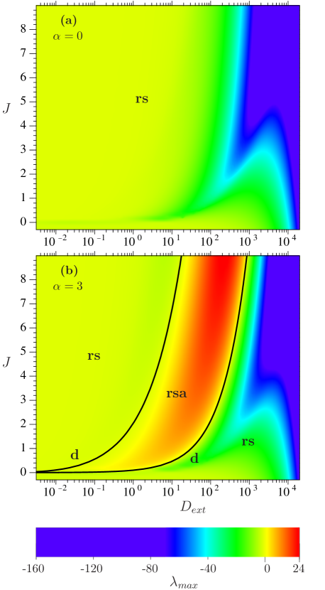
Figure 5: Bifurcation diagram for the white noise forced laser model (18–19) in the $(D_{ext},J)$-plane for (a) $\alpha=0$ and (b) $\alpha=3$. rs stands for random sink, rsa stands for random strange attractor, the two black curves d denote stochastic d-bifurcation, and colour coding is for $\lambda_{max}$. An unforced laser has a Hopf bifurcation at $(D_{ext}=0,J=0)$. Adapted from WIE09 with permission.

Figure 6: Pullback convergence to (a–c) a random sink for $D_{ext}=0.1$ and (d–f) a random strange attractor for $D_{ext}=0.5$ in the white noise forced laser model (18–19) with $\alpha=3$ and $J=1$. Shown are snapshots of $10\,000$ trajectories in projection onto the complex $E$-plane at time $t=30$. The initial conditions are uniformly distributed on the $E$-plane with $N=0$ at different initial times $t_{0}$=(a,d) 29, (b,e) 28, and (c,f) 0.

VI Synchronisation transitions via Stochastic d-bifurcation

To facilitate the analysis we make use of Definitions 1–3 and, henceforth, consider noise synchronisation in the laser model with white noise external forcing

$$\frac{dE}{dt} = i\Delta\,E+g\gamma(1-i\alpha)NE+f_{ext}(t),$$ (18)

$$\frac{dN}{dt} = J-N-(1+gN)|E|^{2},$$ (19)

but without the intrinsic spontaneous emission noise. Now, owing to the absence of intrinsic noise, Definition 4 is equivalent to the synchronisation detection scheme chosen in Section IV. More specifically, the evolution of $M$ trajectories starting at different initial conditions for a single laser with external forcing is the same as the evolution of an ensemble of $M$ identical uncoupled lasers with the same forcing, where each laser starts at a different initial condition. A random sink for (18–19) in the form of a unique attracting trajectory, $a(t,f_{ext})$, makes trajectories for different initial conditions converge to each other. In an ensemble of $M$ identical uncoupled lasers with common forcing this means that $\langle I_{M}\rangle\rightarrow M^{2}\langle I_{fr}\rangle$ in time so that synchronisation is detected. A random strange attractor for (18–19), where nearby trajectories separate exponentially fast because $\lambda_{max}>0$, implies $\langle I_{M}\rangle<M^{2}\langle I_{fr}\rangle$ so that incomplete synchronisation or lack of synchronisation is detected.

Figure 5 shows effects of white noise external forcing on the sign of the otherwise zero $\lambda_{max}$ in an unforced laser. For $\alpha=0$, external forcing always shifts $\lambda_{max}$ to negative values meaning that the system has a random sink for $D_{ext}>0$ and $J>0$ [Fig. 5(a)]. Additionally, this random sink is a unique trajectory, $a(t,f_{ext})$, meaning that the laser is synchronised to white noise external forcing. However, for $\alpha=3$ there are two curves of stochastic d-bifurcation where $\lambda_{max}$ crosses through zero [Fig. 5(b)]. Noise synchronisation is lost for parameter settings between these two curves, where $\lambda_{max}>0$ indicates a random strange attractor . Pullback convergence to two qualitatively different random attractors found for $\alpha=3$ is shown in Fig. 6. At fixed time $t=30$, we take snapshots of $10\,000$ trajectories for a grid of initial conditions with different initial times $t_{0}$. In (a–c), trajectories converge in the pullback sense to a random sink. The random sink appears in the snapshots as a single dot whose position is different for different $t$ or different noise realisations $f_{ext}$. In (d–f), trajectories converge in the pullback sense to a random strange attractor that appears in the snapshots as a fractal-like structure. This structure remains fractal-like but is different for different $t$ or different noise realisations $f_{ext}$.

VI.1 Class-B Laser Model vs. Landau-Stuart Equations

The stochastic d-bifurcation uncovered in the previous section has been reported in biological systems KOS04 ; GOL05 ; GOL06 ; LIN07 ; LIN08 and should appear in a general class of oscillators with stochastic forcing. Here, we use the laser model in conjunction with the Landau-Stuart model to address its dependence on the three parameters: $D_{ext},J,$ and $\alpha$, and to uncover its universal properties. With an exception of certain approximations GOL06 , this problem is beyond the reach of analytical techniques and so numerical analysis is the tool of choice.

To help identifying effects characteristic to the more complicated laser model, we first consider the Landau-Stuart model with white noise external forcing

$$\frac{dE}{d\tilde{t}}=\left[J+i\left(\tilde{\Delta}-\alpha(J-|E|^{2})\right)\right]E-E|E|^{2}+f_{ext}(\tilde{t}),$$ (20)

where, for the rescaled time $\tilde{t}$, the external forcing correlations become

$$\langle f_{ext}^{R}(\tilde{t})f_{ext}^{R}(\tilde{t}^{\prime})\rangle=\langle f_{ext}^{I}(\tilde{t})f_{ext}^{I}(\tilde{t}^{\prime})\rangle=\frac{D_{ext}}{g\gamma}\delta(\tilde{t}-\tilde{t}^{\prime}).$$

Figure 7(a–b) shows the dependence of the d-bifurcation on $J$, $D_{ext}$, and $\alpha$ in Eq. (20). In the three-dimensional $(J,D_{ext},\alpha)$-parameter space, the two-dimensional surface of d-bifurcation appears to originate from the half line $(D_{ext}=0,J=0,\alpha>5.3)$ of the deterministic Hopf bifurcation, has a ridge at $\alpha_{min}\approx 5.3$, and is asymptotic to $\alpha\approx 9$ with increasing $D_{ext}$ [Fig. 7(b)]. Furthermore, numerical results in Fig. 7(b) suggest that the shape of the d-bifurcation curve in the two-dimensional section $(D_{ext},\alpha)$ is independent of $J$. As a consequence, for fixed $\alpha$ within the range $\alpha\in(5.3,9)$ one finds two d-bifurcation curves in the $(D_{ext},J)$-plane [Fig. 7(a)] that are parametrised by

$$J_{j}=C_{j}(\alpha)\sqrt{2D_{ext}}\,\,,\;\;\;\;\mbox{where}\;\;\;\;j=1,2,$$ (21)

Figure 7: A three-parameter study of stochastic d-bifurcation (a–b) in the white noise forced Landau-Stuart model (20) and (c–d) the white noise forced laser model (18–19). To facilitate the comparison between (20) and (18–19), we plotted results for (18–19) with the rescaled forcing strength, $\sqrt{2D_{ext}/g\gamma}$. Adapted from WIE09 with permission.

and bound the region with a random strange attractor. Since $C_{1}(\alpha_{min})=C_{2}(\alpha_{min})=1$, these two curves merge into a single curve

$$J=\sqrt{2D_{ext}}\,\,,$$ (22)

when $\alpha=\alpha_{min}$. On the one hand, for $\alpha\leq\alpha_{min}$, the region with a random strange attractor disappears from the $(D_{ext},J)$-plane. On the other hand, for $\alpha>9$, there is just one d-bifurcation curve in the $(D_{ext},J)$-plane, meaning that the region with a random strange attractor becomes unbounded towards increasing $D_{ext}$ [Fig. 7(b)].

Similar results are expected for any white noise forced oscillator with shear that is near a Hopf bifurcation, and for ’weak’ forcing. This claim is supported with numerical analysis of the laser model (18–19) in Fig. 7(c–d). For a fixed $\alpha$, Eq. (20) and Eqs. (18–19) give identical results if the forcing is weak enough but significant discrepancies arise with increasing forcing strength. First of all, it is possible to have one-dimensional sections of the $(D_{ext},J)$-plane for fixed $J$ with multiple uplifts of $\lambda_{max}$ to positive values [black dots for $J<10^{-6}$ in Fig. 7(c)]. Secondly, the parameter region with a random strange attractor for Eqs. (18–19) expands towards much lower values of $\alpha>\alpha_{min}\approx 1$ [Fig. 7(d)]. Thirdly, the shape of the two-dimensional surface of d-bifurcation in the laser model becomes dependent on $J$ and has a minimum rather than a ridge. As a consequence, although the stochastic d-bifurcation seems to originate from the half line $(D_{ext}=0,J=0,\alpha>5.3)$, it will appear in the $(D_{ext},J)$-plane even for $\alpha\in(1,5.3)$ as a closed and isolated curve away from the origin of this plane [Fig. 7(c)]. Finally, the region of random strange attractor remains bounded in the $(D_{ext},J)$-plane even for large $\alpha$.

Figure 8: $J$ versus (solid) the two non-zero Lyapunov exponents, $\mbox{Re}(\mu_{2})$ and $\mbox{Re}(\mu_{3})$, for the limit cycle in the laser model (1–2), and (dashed) the nonzero Lyapunov exponent, $\mu_{2}$, for the limit cycle in the Landau-Stuart model (5). Adapted from WIE09 with permission.

To unveil the link between the transient dynamics of unforced systems and the forcing-induced stochastic d-bifurcation, we plot $J$ versus Lyapunov exponents in Fig. 8; note that Lyapunov exponents, $\lambda_{i}$, and Floquet exponents, $\mu_{i}$, are related by $\lambda_{i}={\textrm{R}e}[\mu_{i}]$. A comparison between Figs. 7 and 8 shows strong correlation between the relaxation towards the limit cycle and the d-bifurcation. In the Landau-Stuart model (5), the linear relation (6) between $J$ and the non-zero Lyapunov exponent, $\mu_{2}$ (dashed line in Fig. 8), results in a linear parametrisation (21) of d-bifurcation curves in the ($J,\sqrt{2D_{ext}})$-plane [Fig. 7(a)]. In the laser model (1–2), the nonlinear relation (3–4) between $J$ and the non-zero Lyapunov exponents, $\mbox{Re}(\mu_{2})$ and $\mbox{Re}(\mu_{3})$ (solid curves in Fig. 8), results in a very similar nonlinear parametrisation of d-bifurcation curves in the ($J,\sqrt{2D_{ext}}$)-plane [Fig. 7(c)]. The splitting up of the chaotic region bounded by the black dots for $J<9\times 10^{5}$ in Fig. 7(c) is related to two different eigendirections normal to the limit cycle with significantly different timescales of transient dynamics towards the limit cycle (the two corresponding Lyapunov exponents are shown in solid in Fig. 8). Finally, the appearance of relaxation oscillations in the laser system is associated with a noticeable expansion of the chaotic region, in particular, towards smaller $\alpha$.

VII Noise-induced strange attractors

Complicated invariant sets, such as strange attractors, require a balanced interplay between phase space expansion and contraction GUC83 . If phase space expansion in certain directions is properly compensated by phase space contraction in some other directions, nearby trajectories can separate exponentially fast ($\lambda_{max}>0$) and yet remain within a bounded subset of the phase space.

It has been recently proven that, when suitably perturbed, any stable hyperbolic limit cycle can be turned into ‘observable’ chaos (a strange attractor) WAN03 . This result is derived for periodic discrete-time perturbations (kicks) that deform the stable limit cycle of the unkicked system. The key concept is the creation of horseshoes via a stretch-and-fold action due to an interplay between the kicks and the local geometry of the phase space. Depending on the degree of shear, quite different kicks are required to create a stretch-and-fold action and horseshoes. Intuitively, it can be described as follows. In systems without shear, where points in phase space rotate with the same angular frequency about the origin of the complex $E$-plane independent of their distance from the origin, the kick alone has to create the stretch-and-fold action. This is demonstrated in Fig. 9. Horseshoes are formed as the system is suitably kicked in both radial and angular directions and then relaxes back to the attractor [the circle in Fig. 9(a)] of the unkicked system. Repeating this process reveals chaotic invariant sets. However, showing rigorously that a specific kick results in ‘observable’ chaos is a non-trivial task WAN03 . In the presence of shear, where points in phase space rotate with different angular frequencies depending on their distance from the origin, the kick does not have to be so specific or carefully chosen. In fact, it may be sufficient to kick non-uniformly in the radial direction alone, and rely on natural forces of shear to provide the necessary stretch-and-fold action.

These effects are illustrated in Fig. 10 for the single laser model (1–2) with non-uniform kicks in the radial direction alone for $\alpha=0$ (no shear) and $\alpha=2$ (shear). There, we set $\Delta=0$ and refer to the stable limit cycle [dashed circle in Fig. 10(a)] as $\Gamma$. Kicks modify the electric field amplitude, $|E|$, by a factor of $0.8\sin[4\,\arg(E)]$ at times $t=0,\,0.25,\,0.5,\,\mbox{and}\,0.75$, but leave the phase, $\arg(E)$, unchanged. For $\alpha=0$ each point on the black curve spirals onto $\Gamma$ in time but remains within the same isochrone defined by a constant electric-field phase, $\arg(E)=\arg(E(0))$. Hence, the black curve does not have any folds at any time. However, for $\alpha=2$, a kick moves most points on the black curve to different isochrones so that points with larger amplitudes $|E|$ rotate with larger angular frequencies. This gives rise to an intricate stretch-and-fold action. Folds and horseshoes can be formed under the evolution of the flow even though the kicks are in the radial direction alone.

Figure 9: Time evolution of sets of initial conditions showing the creation of horseshoes in the phase space of a suitably kicked laser model with no shear ($\alpha=0$). The sets of initial conditions are (a) the stable circle and (d) boxes containing parts of the circle. Shown are phase portraits [(a) and (d)] before, [(b) and (e)] immediately after the first kick, and [(c) and (f)] some time after the first kick.

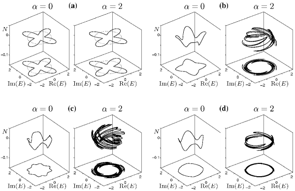
Figure 10: Snapshots at times (a) $t=0$, (b) $t=0.35$, (c) $t=0.8$, and (d) $t=1$ showing the time evolution of $15000$ trajectories with initial conditions distributed equally over the stable circle for (1–2). Kicks in the radial direction alone are applied at times $t=0,0.25,0.5,0.75$. A comparison between $\alpha=0$ and $\alpha=2$ illustrates the $\alpha$-induced stretch-and-fold action in the laser phase space.

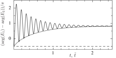
Figure 11: Phase-space stretching along the limit cycle shown as time evolution of the phase difference between two trajectories starting at different isochrones. The three curves are obtained using (dashed) Eqs. (1–2) with $\alpha=0$, (solid) Eqs. (1–2) with $\alpha=3$, and (dotted) Eq. (5) with $\alpha=3$. Adapted from WIE09 with permission.

In the laser model, stretch-and-fold action is significantly enhanced by the spiralling transient motion about $\Gamma$. For $J>10^{-1}$, the laser model (1–2) and the Landau-Stuart model (5) have nearly identical relaxation timescales toward $\Gamma$ (Fig. 8). However, owing to one additional degree of freedom and oscillatory relaxation (4), the instantaneous stretching along $\Gamma$ in the three-dimensional laser vector field (1–2) can be much stronger compared to the planar vector field (5), especially at short times after the perturbation. This effect is illustrated in Fig. 11 by the time evolution of the phase difference, $\arg(E_{1}(t))-\arg(E_{2}(t))$, between two trajectories, 1 and 2, starting at different isochrones for $\alpha=3$. Since both vector fields have identically shaped isochrones (8), the phase difference converges to the same value as time tends to infinity. However, at small $t$, the oscillatory phase difference for (1–2) can exceed significantly the monotonically increasing phase difference for (5) (compare solid and dotted curves in Fig. 11).

It is important to note that the rigorous results for turning stable limit cycles into chaotic attractors are derived for periodic discrete-time perturbations. Stochastic forcing is a continuous-time perturbation, meaning that the analysis in WAN03 cannot be directly applied to our problem. Nonetheless, such analysis gives a valuable insight as to why random chaotic attractors appear for $\alpha$ sufficiently large, and it helps distinguish effects of stochastic forcing.

Here, we demonstrated that purely additive white noise forcing is sufficient to induce random strange attractors in limit cycle oscillators. Furthermore, numerical analysis in Sec. VI.1 shows that, in the case of stochastic forcing, creation of strange attractors requires a different balance between the amount of shear, relaxation rate toward the limit cycle, and forcing strength, as compared to periodic forcing. Unlike in the case of discrete-time periodic forcing, the shear has to be strong enough, $|\alpha|>C>0$, to allow sufficient stretch-and-fold action. Provided that the shear is strong enough, the stochastic forcing strength needs to be at least comparable to the relaxation rate toward the limit cycle to allow formation of random strange attractors. Furthermore, we demonstrated that in higher dimensional systems, different eigendirections with distinctly different relaxation rates toward the limit cycle could give rise to more than one region in the ($J,\sqrt{2D_{ext}}$)-plane with a random strange attractor. Last but not least, we revealed that the enhancement in the instantaneous stretch-and-fold action arising from laser relaxation oscillations results in a larger parameter region with a random strange attractor.

VIII Conclusions

We used the class-B laser model in conjunction with the Landau-Stuart model (Hopf normal form with shear) to study noise synchronisation and loss of synchrony via shear-induced stochastic d-bifurcations.

We defined noise synchronisation in terms of pullback convergence of random attractors and showed that a nonlinear oscillator can synchronise to stochastic external forcing. However, the parameter region with synchronous dynamics becomes interrupted with a single or multiple intervals of asynchronous dynamics if amplitude-phase coupling or shear is sufficiently large. Stability analysis shows that the synchronous solution represented by a random sink loses stability via stochastic d-bifurcation to a random strange attractor. We performed a systematic study of this bifurcation with dependence on the three parameters: the Hopf bifurcation parameter (laser pump), the amount of shear (laser linewidth enhancement factor), and the stochastic forcing strength.

In this way, we uncovered a vast parameter region with random strange attractors that are induced purely by stochastic forcing. More specifically, in the three-dimensional parameter space, the two-dimensional surface of the stochastic bifurcation originates from the half-line of the deterministic Hopf bifurcation. In the plane of stochastic forcing strength and Hopf bifurcation parameter, one finds stochastic d-bifurcation curve(s) bounding region(s) of random strange attractors if the amount of shear is sufficiently large. The shape of d-bifurcation curves is determined by the type and rate of the relaxation toward the limit cycle in the unforced oscillator. Near the Hopf bifurcation and provided that stochastic forcing is weak enough, the d-bifurcation curves satisfy the numerically uncovered power law (21). However, as the stochastic forcing strength increases, there might be deviations from this law. The deviations arise because different oscillators experience different effects of higher-order terms and additional degrees of freedom on the relaxation toward the limit cycle. In the laser example, the d-bifurcation curves deviate from the simple power law (21) so that the region of a random strange attractor splits up and expands toward smaller values of shear as the forcing strength increases. We intuitively explained these results by demonstrating that the shear-induced stretch-and-fold action in the oscillator’s phase space facilitates creation of horseshoes and strange attractors in response to external forcing. Furthermore, we showed that the stretch-and-fold action can be greatly enhanced by damped relaxation oscillations in the laser model, causing the deviation from the simple power law.

References

- (1) A.S. Pikovsky, M. Rosenblum, and J. Kurths, Synchronisation-a unified approach to nonlinear science, Cambridge University Press, Cambridge, 2001.
- (2) A.S. Pikovsky,in Nonlinear and turbulent processes in physics, edited by R.Z. Sagdeev (Harwood Academic, Singapore, 1984), 1601–1604.
- (3) Z.F. Mainen and T.J. Sejnowski, “Reliability of spike timing in neocortical neurons”, Science 268 1503–1506 (1995).
- (4) R.V. Jensen, “Synchronization of randomly driven nonlinear oscillators”, Phys. Rev. Lett. 58 R6907–R6910 (1998).
- (5) C.S. Zhou, J. Kurths, E. Allaria, S. Boccaletti, R. Meucci, and F. T. Arecchi, “Constructive effects of noise in homoclinic chaotic systems”, Phys. Rev. Lett. 67 066220 (2003).
- (6) J. Teramae and D. Tanaka, “Robustness of the Noise-Induced Phase Synchronization in a General Class of Limit Cycle Oscillators”, Phys. Rev. Lett. 93 204103 (2004).
- (7) A. Uchida, R. McAllister, and R. Roy, “Consistency of nonlinear system response to complex drive signals”, Phys. Rev. Lett. 93 244102 (2004).
- (8) E. Kosmidis and K. Pakdaman, “ An Analysis of the Reliability Phenomenon in the FitzHugh-Nagumo Model”, J. Comp. Neurosci. 14 5–22 (2003).
- (9) D.S. Goldobin and A. Pikovsky, “Synchronisation and desynchronisation of self-sustained oscillators by common noise”, Phys. Rev. E 71 045201(R) (2005).
- (10) D.S. Goldobin and A. Pikovsky, “Antireliability of noise-driven neurons”, Phys. Rev. E 73 061906 (2006).
- (11) N.F. Rulkov, M.M. Sushchik, L.S. Tsimring, and H.D.I. Abarbanel, “Generalised synchronisation of chaos in directionally coupled chaotic systems”, Phys. Rev. E 51 980–994 (1995).
- (12) S. Wieczorek “Stochastic bifurcation in noise-driven lasers and Hopf oscillators”, Phys. Rev. E 79 036209 (2009).
- (13) K.K. Lin, E. Shea-Brown, and L.-S. Young, “Reliability of coupled oscillators”, J. Nonlin. Sci. 19 497–545 (2009).
- (14) K.K. Lin, and L.-S. Young, “Shear-induced chaos”, Nonlinearity 21 899–922 (2008).
- (15) S. Wieczorek, B. Krauskopf, T.B. Simpson, and D. Lenstra, “The dynamical complexity of optically injected semiconductor lasers”, Phys. Rep. 416 1–128 (2005).
- (16) S. Wieczorek and W.W. Chow, “Bifurcations and chaos in a semiconductor laser with coherent or noisy optical injection”, Optics Communications 282 (12) 2367–2379 (2009).
- (17) J. Guckenheimer and P. Holmes, Nonlinear oscillations, dynamical systems, and bifurcations of vector fields, Springer-Verlag, New York 1983.
- (18) C.H. Henry, “Theory of the linewidth of semiconductor laser”, IEEE J. Quantum Electron. QE–18 259 (1982).
- (19) J. Guckenheimer, “Isochrons and phaseless sets”, J. Math. Biol. 3 259–273 (1974/75).
- (20) R. Lang, “Injection locking properties of a semiconductor laser”, IEEE J. Quantum Electron. 18, 976 (1982).
- (21) W.W. Chow, M.O. Scully, and E.W. van Stryland, “Line narrowing in a symmetry broken laser”, Opt. Commun. 15 6–9 (1975).
- (22) T. Erneux, V. Kovanis, A. Gavrielides, and P.M. Alsing, “Mechanism for period-doubling bifurcation in a semiconductor laser subject to optical injection”, Phys. Rev. A 53 4372–4380 (1996).
- (23) K.E. Chlouverakis and M.J. Adams, “Stability map of injection-locked laser diodes using the largest Lyapunov exponent”, Opt. Comm. 216 405–412 (2003).
- (24) C. Bonatto and J.A.C. Gallas, “Accumulation horizons and period adding in optically injected semiconductor lasers”, Phys. Rev. E 75 055204R (2007).
- (25) S. Wieczorek, T.B. Simpson, B. Krauskopf, and D. Lenstra “Global quantitative predictions of complex laser dynamics”, Phys. Rev. E 65 045207R (2002).
- (26) L. Arnold, Random Dynamical Systems, (Springer-Verlag, Berlin Heidelberg, 1998).
- (27) P. Ashwin and G. Ochs, “Convergence to local random attractors”, Dyn. Syst. 18 (2) 139–158 (2003).
- (28) N.F. Rulkov, M.M. Sushchik, L.S. Tsimring, and H.D.I. Abarbanel, “Generalised synchronisation of chaos in directionally coupled chaotic systems”, Phys. Rev. E 51 (2) 980–994 (1995).
- (29) H.D.I. Abarbanel N.F. Rulkov, and M.M. Sushchik, “Generalised synchronisation of chaos: The auxiliary system approach”, Phys. Rev. E 53 (5) 4528–4535 (1996).
- (30) K. Pyragas, “Weak and strong synchronisation of chaos”, Phys. Rev. E 54 (5) R4508–R4511 (1996).
- (31) R. Brown and L. Kocarev, “A unifying definition of synchronisation for dynamical systems”, Chaos 10 (2) 344–349 (2000).
- (32) J.A. Langa, J.C. Robinson, and A. Súarez, “Stability, instability, and bifurcation phenomena in non-autonomous differential equations”, Nonlinearity 15 (2) 1–17 (2002).
- (33) Q. Wang and L.-S. Young, “Strange attractors in periodically-kicked limit cycles and Hopf bifurcations”, Comm. Math. Phys. 240 509–529 (2003).