On the dimerized phase in the cross-coupled antiferromagnetic spin ladder

Abstract

We revisit the phase diagram of the frustrated $s$=1/2 spin ladder with antiferromagnetic rung and diagonal couplings. In particular, we reexamine the evidence for the columnar dimer phase, which has been predicted from analytic treatment of the model and has been claimed to be found in numerical calculations. By considering longer chains and by keeping more states than in previous work using the density-matrix renormalization group, we show that the numerical evidence presented previously for the existence of the dimerized phase is not unambiguous in view of the present more careful analysis. While we cannot completely rule out the possibility of a dimerized phase in the cross-coupled ladder, we do set limits on the maximum possible value of the dimer order parameter that are much smaller than those found previously.

I Introduction

In spin chains, frustration due to competing antiferromagnetic nearest- and comparably strong next-nearest-neighbor coupling leads to the appearance of a new gapped, dimerized phasehald ; affleck whose properties are markedly different from that of the uniform spin-liquid state of the antiferromagnetic spin-1/2 chain. A much richer phase diagram is found in spin ladders, where the couplings between nearest-neighbor spins situated along the legs and on the rungs of the ladder may compete. These phases and the quantum phase transitions between them have been extensively studied recently, both experimentally and theoretically.frustrated The theoretical approaches include both analytic and numerical work. The analytic treatment of the bosonized form of the spin Hamiltonian has been widely used to predict the phase diagram. cg ; shelton ; nt ; chp ; og ; weihong ; nge ; gt ; aen ; gene ; oleg There is general agreement that, in two-leg spin ladders, the most relevant operator generates either a topologically ordered rung-singlet or a Haldane phase, depending on the relative strength of the intraleg and interleg couplings.

The competition between the couplings is, however, a delicate problem when the intraleg and the interleg couplings are of the same order of magnitude, and the type of order is, in some cases, determined by marginally relevant terms generated within the renormalization group (RG) procedure. Among the many terms generated, operators leading to dimerization appear. On this basis,oleg it was proposed that a dimerized phase appears between the topologically ordered rung-singlet and the Haldane phases for the so-called cross-coupled ladder, in which spins are coupled not only along the legs and across the rungs but also diagonally, i.e., on opposite legs and on different, neighboring rungs.

The existence of an analogous dimerized phase induced by four-spin exchange terms has been proposed some time ago.nt This dimerized phase has indeed been found to exist numerically.lfs ; kolezhuk ; pati ; muller ; lauchli ; momoi It is also well-established that a dimerized phase exists when a second-neighbor interaction on the legs of the ladder are present honecker or when the interleg coupling is ferromagnetic.hikihara The existence of the dimerized phase has, however, been disputed for ladders with pairwise spin interactions only,wang ; hung ; kim2008 while other work has presented evidence supporting the presence of this phase.liu ; hikihara

The density-matrix renormalization group (DMRG) procedure invented by Whitewhite is a particularly useful numerical method to study such problems because it makes possible the high-precision calculation of the ground-state properties and low-lying excitations of low-dimensional quantum systems. The DMRG has indeed been widely used lfs ; fath ; hf ; hhr ; fouet ; meyer ; sheng to explore the possible phases of spin ladders. The length of the ladders from which finite-size scaling is done and the accuracy of the DMRG calculation can be, however, decisive. Motivated mainly by the recent work of Hikihara and Starykhhikihara , we have undertaken a careful analysis of the numerical data to see if there is indeed compelling evidence for the dimerized phase in the cross-coupled ladder using the DMRG procedure.

The paper is organized as follows. In Sec. II, we summarize earlier results on the phase diagram of the cross-coupled frustrated antiferromagnetic spin-1/2 ladder. The aspects of the DMRG procedure that determine its accuracy are briefly discussed in Sec. III. Our numerical results are presented in Sec. IV. Finally Sec. V contains our conclusions.

II Previous results on the cross-coupled spin ladder

We treat a two-leg spin-1/2 ladder with pairwise Heisenberg couplings along the legs, across the rungs, and diagonally between sites on adjacent rungs, but on opposite legs. The Hamiltonian can be written

$${\mathcal{H}}=\sum_{i}{\mathcal{H}}_{i,i+1}\,,$$ (1)

where

$${\mathcal{H}}_{i,i+1} = J_{\|}\left(\boldsymbol{S}_{1,i}\cdot\boldsymbol{S}_{1,i+1}+\boldsymbol{S}_{2,i}\cdot\boldsymbol{S}_{2,i+1}\right)$$

$$+\textstyle{\frac{1}{2}}J_{\bot}\left(\boldsymbol{S}_{1,i}\cdot\boldsymbol{S}_{2,i}+\boldsymbol{S}_{1,i+1}\cdot\boldsymbol{S}_{2,i+1}\right)$$

$$+J_{\times}\left(\boldsymbol{S}_{1,i}\cdot\boldsymbol{S}_{2,i+1}+\boldsymbol{S}_{2,i}\cdot\boldsymbol{S}_{1,i+1}\right)\,,$$

and $\boldsymbol{S}_{1,i}$ and $\boldsymbol{S}_{2,i}$ are the spin operators on rung $i$ and legs 1 and 2, respectively. A depiction of the couplings of the cross-coupled ladder is shown in Fig. 1.

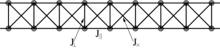
Figure 1: (Color online) Depiction of the cross-coupled ladder.

Here we will consider only antiferromagnetic coupling and set the intraleg coupling to unity, $J_{\|}=1$ which we take as the energy scale in the problem. For $J_{\times}=0$, it has been established that the entire half-line $0<J_{\bot}<\infty$ of the ground-state phase diagram, is continuously connected,wns ; shelton i.e., no phase transition occurs for any finite value of $J_{\bot}$. Since the configuration that dominates the ground-state wave function is the product of rung singlets, this phase is often referred to as the rung-singlet (RS) phase. Conversely, for $J_{\bot}=0$, the entire half-line $0<J_{\times}<\infty$ is continuously connected to the Haldane phase haldane of the spin-1 chain and the system is known to have a gapped spectrum of spin-1 magnons. lfs ; ls

When both $J_{\bot}$ and $J_{\times}$ are finite, frustration due to competition between the intraleg and the rung or diagonal interleg couplings potentially leads to the formation of new phases. Indications for such new phases are given by analytic calculations which can be performed for weak interchain couplings using the bosonized form of the Hamiltonian. The leading term in the Hamiltonian is the coupling between the staggered magnetizations of the legs:

$$(J_{\bot}-2J_{\times})\boldsymbol{n}_{1}\cdot\boldsymbol{n}_{2}\,.$$ (3)

This term generates a gap in the spectrum irrespective of the sign of the coefficient $J_{\bot}-2J_{\times}$. Rung singlets are generated for $J_{\bot}-2J_{\times}>0$, while the Haldane phase appears for $J_{\bot}-2J_{\times}<0$. The first numerical results on the model weihong ; fath were consistent with a first-order transition for both weak and strong interchain couplings. Subsequent work has suggested that the transition is actually continuous when the interchain coupling is weak, becoming first-order only for stronger interchain coupling.wang ; hung This scenario has been supported further by an analysis based on quantum information entropies.kim2008 Although two critical values of the coupling were found in the two-site entropy function for finite systems in this work, it was shown that they scale to a single value in the thermodynamic limit. It was therefore argued that a direct transition between the rung singlet and the Haldane phases takes place.

When $J_{\bot}=2J_{\times}$, the most relevant term is suppressed at the transition between the two gapped phases and other, less relevant terms may play a role. In particular, such terms lead to the prediction of a spontaneously dimerized phase.oleg ; kim2008 ; hikihara The boundaries of this dimerized phase have been estimated to lie at

$$J_{\bot}=2J_{\times}-\frac{5}{\pi^{2}}J^{2}_{\times}\quad\mbox{and}\quad J_{\bot}=2J_{\times}-\frac{1}{\pi^{2}}J^{2}_{\times}\,.$$ (4)

The most recent numerical results, however, indicate a much narrower range for the existence of the dimerized phase.liu ; hikihara In Ref. liu, the dimerized phase was claimed to exist in the range $0.373\leq J_{\bot}\leq 0.386$ for $J_{\times}=0.2$. The authors of Ref. hikihara, chose a single point in the middle of this range, namely $J_{\bot}=0.38$, $J_{\times}=0.2$ to demonstrate the existence of the dimerized phase. In what follows, we will also restrict ourselves to the vicinity of this single point in parameter space and will carry out a careful numerical analysis of the dimer order parameter in the range $0.36\leq J_{\bot}\leq 0.4$ for $J_{\times}=0.2$.

III Numerical procedure

III.1 Factors determining the accuracy of the DMRG procedure

In the standard DMRG procedure, the chain is divided into two blocks and two extra sites. As the two sites are incorporated into larger blocks during the steps of the renormalization procedure, only a fraction of the new block states are kept; the others are discarded. Usually the number of block states, $M$, kept in the truncation procedure ranges from a few hundred to a few thousand and is set according to the accuracy required and the available computational resources.schollwock ; manmana ; hallberg

As we have pointed out in previous work, keeping the number of block states constant for increasingly large system sizes leads to increasing error, legeza02 ; legeza03 i.e., the scaling of block entropy with system size is not taken into account.vidal03 In a consistent calculation, the number of block states must be increased as system size is increased. The finite-size scaling to infinite system size must be accompained by a systematic increase of $M$, and the $M\rightarrow\infty$ limit must be taken. We have shown that the proper choice of $M$ can be determined by the so-called Dynamic Block State Selection (DBSS) approach,legeza02 ; legeza03 in which the threshold value of the quantum information loss $\chi$ is fixed a priori. In this approach, the number of block states to be kept is obtained from the criterion $s-s^{\rm Trunc}\leq\chi$, where $s$ and $s^{\rm Trunc}$ stand for the block entropy before and after the truncation, respectively. The minimum number of block states $M_{\rm min}$ is set prior to the calculation, and the maximum number of block states needed to achieve the desired accuracy, $M_{\rm max}$, is monitored during the DMRG process. This allows for a rigorous control of the numerical accuracy and gives a stable extrapolation to $\chi=0$.

III.2 Choice of a proper order parameter: advantages and limitations

In an earlier workgene we used the generalization of the so-called hidden topological order,dennijs $O$, to two-leg ladders,

$${\mathcal{O}}_{\text{odd}} = -\lim_{|i-j|\rightarrow\infty}\Bigg{\langle}(S_{i,1}^{z}+S_{i,2}^{z})$$

$$\times\exp\left[i\pi\sum_{l=i+1}^{j-1}(S_{l,1}^{z}+S_{l,2}^{z})\right](S_{j,1}^{z}+S_{j,2}^{z})\Bigg{\rangle}\,,$$

and

$${\mathcal{O}}_{\text{even}} = -\lim_{|i-j|\rightarrow\infty}\Bigg{\langle}(S_{i+1,1}^{z}+S_{i,2}^{z})$$

$$\times\exp\left[i\pi\sum_{l=i+1}^{j-1}(S_{l+1,1}^{z}+S_{l,2}^{z})\right](S_{j+1,1}^{z}+S_{j,2}^{z})\Bigg{\rangle}\,,$$

to identify various spin-liquid phases.fath The advantage of these specially constructed order parameters is that only one of them can be finite in a given phase and they both vanish for critical systems. Unfortunately, the rung-singlet and dimerized phases would fall into the same topological sector because $O_{\rm even}$ is finite for both cases. Thus, they cannot be distinguished by the topological order.

A similar problem arises for the so-called $z$ operators,nakamura01 ; nakamura02 which can also be used to distinguish different odd- or even-parity valence-bond-solid (VBS) states. The operator

$$z_{\text{rung}}=\left\langle\exp\left[i\frac{2\pi}{N}\sum_{l=1}^{N}l(S_{1,l}^{z}+S_{2,l}^{z})\right]\right\rangle\,,$$ (7)

defined for ladders with periodic boundary conditions, converges to $+1$ in the rung-singlet phase and to $-1$ in the Haldane phase, while the operator

$$z_{\text{diag}}=\left\langle\exp\left[i\frac{2\pi}{N}\sum_{l=1}^{N}l(S_{1,l+1}^{z}+S_{2,l}^{z})\right]\right\rangle$$ (8)

converges to $-1$ and $+1$, respectively, in the two topologically distinct phases. They give a clear indication of the parity of the number of singlet bonds “cut” by a line between adjacent rungs, but they do not distinguish between the columnar-dimer phase and the rung-singlet phase.

Since we are looking for a possible columnar-dimer phase only, a more natural quantity to examine is the local dimer order parameter $(D)$ defined as

$$D=\lim_{N\to\infty}|D(N)|$$ (9)

with

$$D(N)=\langle{\cal H}_{N/2-1,N/2}\rangle-\langle{\cal H}_{N/2,N/2+1}\rangle\,.$$ (10)

Thus, dimerization is measured as the alternation in the bond energy in the middle of a sufficiently long open chain. Here $D$ is finite when the translational symmetry of the Hamiltonian is spontaneously broken in the thermodynamic limit. It is worth noting that our definition is slightly different from the one used in Ref. hikihara, for the columnar phase, where only the intraleg part of the spin couplings was included. Although, quantitatively the two definitions give different values for the order parameter, the qualitative behavior is the same.

For noncritical models with a finite correlation length, the end effects decay exponentially and the local quantity $D(N)$ is expected to vary to leading order as

$$D(N)=D+aN^{-\beta}\exp(-N/2\xi).$$ (11)

This behavior is qualitatively similar to the scaling of the gap for periodic boundary conditions (PBC), except that the scaling variable is the distance of the middle of the chain from the boundary, $N/2$, and the exponent $\beta$ of the algebraic prefactor is, a priori, unknown. Here $\xi$ stands for the correlation length, which is finite for gapped systems. The exponential convergence of local quantities such as the dimer order parameter $D(N)$ makes the extrapolation to the thermodynamic limit more reliable.buchta2005 In cases when the available data for $D(N)$ not show a tendency to go to a finite value as a function of $1/N$, we also carry out extrapolations without the exponential term in Eq. (11). In addition, in order to obtain an upper bound for $D$, we also use a second order polynomial fit in $1/N$. Since the numerical accuracy is of crucial importance in the present study, we analyze the behavior of the dimer order parameter as a function of $M$ and $\chi$ systematically.

IV Numerical results

As mentioned above, the dimerized phase exists, if it exists at all, in a narrow region around $J_{\bot}=0.38,J_{\times}=0.2$. We first calculate the length-dependent $D(N)$ using open boundary conditions (OBC) on systems of up to $N=512$ rungs in steps of $32$. We perform four DMRG sweeps with fixed numbers of block states, $M=256$ and $512$. Note that the longest system studied in Ref. hikihara, had $N=192$ rungs. The results for the dimer order parameter at $J_{\bot}=0.38,J_{\times}=0.2$ are shown on a log-log scale in Fig. 2 to allow for direct comparison with Fig. 10 of Ref. hikihara, .

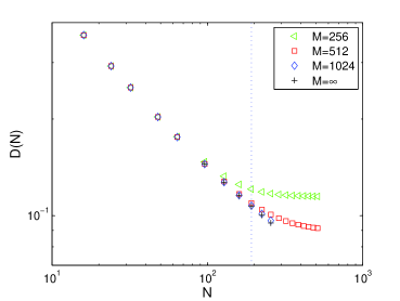
Figure 2: (Color online) Dimer order parameter $D(N)$ plotted as a function of $N$ on a log-log scale for various fixed numbers of block states ($M$) for $J_{\bot}=0.38,J_{\times}=0.2$. The dotted line indicates $N=192$, the largest system studied previously. The $M=\infty$ extrapolation is taken from the fits depicted in Fig. 3(a).

The data points calculated at fixed $M$, $M=256$ or $M=512$, exhibit a clear tendency to go to a finite value as a function of $N$ in the infinite-chains limit. The flat region develops for $M=256$ at chain length ($N\simeq 128$) and for $M=512$ when $N$ exceeds about $256$. This flattening of the dimer order parameter with increasing $N$ was interpreted as evidence for the presence of a dimerized phase.

In order to see what happens for even larger values of $M$, we have carried out calculations keeping $M=1024$ block states for ladders of up to $N=256$ rungs. As can be seen in Fig. 2, the dimer order parameter does not tend to a finite value with $N$ at the available system sizes. To carry out the standard extrapolation scheme, we have fitted the $M$-dependent $D(N)$ for various system sizes as a function of $1/M$ using the function

$$D(M,N)=D(N)+a(N)M^{-\beta(N)}\,,$$ (12)

where $D(N),a(N)$, and $\beta(N)$ are free fitting parameters. These fits are shown in Fig. 3(a).

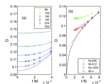
Figure 3: (Color online) (a) Scaling of the dimer order parameter as a function of the number of block states retained, $M$, for various chain lengths. The solid line is a fit using the function $D(M,N)=D+a(N)M^{-\beta(N)}$. (b) The $D(N)$ data of Fig. 2 plotted as a function of $1/N$. The solid line is a fit to the $D(M\rightarrow\infty,N)$ data using Eq. (11). The dotted line is a similar fit without the exponential factor, while the dashed line is a fit to a second-order polynomial in $1/N$.

The finite-size scaling of $D(N)$ can be better seen if this quantity is plotted as a function of $1/N$ rather than as a function of $N$. Such a plot is shown in Fig. 3(b), including $D(M,N)$ for fixed values of $M$. While the data points for $M=256$ and $M=512$ behave as if they would go to a finite value in the $N\rightarrow\infty$ limit, the data available for $M=1024$ ($N\leq 256$) do not show an upward curvature in $1/N$. The same is true for the extrapolated values of the dimer order parameter indicated by the solid line in Fig. 3(b). Extrapolation using Eq. (11) yields $D(M\rightarrow\infty,N\rightarrow\infty)=0.003(2)$ and a very large correlation length, $\xi=5972$. Since a flattening off is not apparent in the curves, we have repeated the fit without the exponential term, yielding $D(M\rightarrow\infty,N\rightarrow\infty)=0.013(5)$. In order to obtain an upper bound for $D$, we have also carried out a fit to a second-order polynomial in $1/N$. The extrapolated value of $D_{\rm ub}(M\rightarrow\infty,N\rightarrow\infty)$ is $0.052(2)$ but this fit, indicated by the dashed line, clearly overestimates the bond order parameter significantly.

By repeating the same analysis for several points in the vicinity of $J_{\bot}=0.38$ keeping $J_{\times}=0.2$ fixed we have also studied the finite-size scaling of $D(N)$ in more detail and determined $D(M\rightarrow\infty,N\rightarrow\infty)$. The results are shown in Fig. 4. For all data points extrapolation using Eq. (11) yields $D(M\rightarrow\infty,N\rightarrow\infty)\simeq\mathcal{O}(10^{-4})$ and a correlation length of the order $10^{2}$, except for $J_{\bot}=0.38$. It is obvious from the figure that the inflection point shows up only at larger system sizes as $J_{\bot}=0.38$ is approached, thus longer and longer systems must be investigated for a reliable extrapolation. It is worth mentioning, however, that in all cases the extrapolated curves start with a horizontal slope.

Figure 4: (Color online) Scaling of $D(M\rightarrow\infty,N)$ as a function of $1/N$ for various $J_{\bot}$ values in the vicinity of $J_{\bot}=0.38$ keeping $J_{\times}=0.2$ fixed. The solid line is a fit to the $D(M\rightarrow\infty,N)$ data using Eq. (11).

Since the decrease of the dimer order parameter is the slowest at $J_{\bot}=0.38$ we have reinvestigated this point using a better extrapolation scheme, i.e., the DBSS method. By setting a limit on the quantum information loss, the number of block states is selected dynamically during the RG steps of the DMRG. In our calculations, the maximum number of block states, $M_{\rm max}$, varies in the range $200-2500$ for decreasing $\chi$. For $\chi=10^{-4}$, we have taken $M_{\rm min}=64$, while we taken $M_{\rm min}=256$ for all other cases. The largest dimension of the superblock Hamiltonian was over 14 million. The number of block states needed to achieve the predetermined $\chi$ value is shown as a function of $1/N$ in Fig. 5(a). Obviously $M_{\rm max}$ diverges for increasing $N$ and decreasing $\chi$. For example, $M\simeq 2500$ states must be kept for a ladder with $N=256$ rungs in order to obtain an accuracy of $\chi=10^{-7}$.

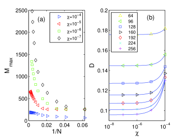
Figure 5: (Color online) (a) Maximum number of block states $M_{\rm max}$ selected dynamically for given accuracy thresholds $\chi$ plotted as a function of inverse system size $1/N$. (b) Scaling of the dimer order parameter as a function of the quantum information loss $\chi$ for various chain lengths.

The dimer order parameter calculated for different accuracy levels is plotted as a function of $\chi$ in Fig.5(b) on a semi-logarithmic scale, while these data and the extrapolated values $D(\chi\rightarrow 0,N)$ are plotted as a function of $1/N$ in Fig. 6(a). Extrapolation to $N\rightarrow\infty$ was again performed using Eq. (11), yielding $D(\chi\rightarrow 0,N\rightarrow\infty)=0.003(1)$, while the fit without the exponential term yielded $D(\chi\rightarrow 0,N\rightarrow\infty)=0.021(5)$. A portion of Fig. 6(a) is displayed in an enlarged scale in Fig. 6(b). It can be clearly seen that a small error, in this case of the order of $10^{-4}$, in $D(\chi\rightarrow 0,N)$ can lead to a significant shift of the extrapolated value. We have again determined an upper bound through a fit to a second-order polynomial in $1/N$, obtaining $D_{\rm ub}(\chi\rightarrow 0,N\rightarrow\infty)=0.054(2)$.

Figure 6: (Color online) (a) Similar to Fig. 3(b) but with data calculated with the indicated fixed values of $\chi$ and extrapolated to $\chi=0$ using an exponential form as shown in 5(b). The solid line is a fit to the $D(N,\chi\rightarrow 0)$ data using Eq. (11). The dotted line is a similar fit without the exponential factor, while the dashed line is a fit to a second-order polynomial in $1/N$. (b) Extrapolated data and fits for an enlarged region.

To compare the results obtained from the $M\rightarrow\infty$ extrapolation with those of the $\chi\rightarrow 0$ extrapolation, we display both $D(M\rightarrow\infty,N)$ and $D(\chi\rightarrow 0,N)$ on the same axes in Fig. 7(a). On the scale used, the results of the two procedures coincide. The difference is of order $10^{-4}$, as can be seen on the logarithmic scale used in Fig. 7 (b). The extrapolated data points show no upward curvature as a function of $1/N$. Thus, we find that there is no evidence for a finite dimer order parameter to the resolution of the calculations performed here.

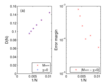
Figure 7: (Color online) (a) Similar to Fig. 3 (b), but with the $M\rightarrow\infty$ and $\chi\rightarrow 0$ extrapolated data plotted on the same scale and (b) their difference plotted on a logarithmic scale as a function of $1/N$.

V Conclusion

In summary, we have carried out density-matrix renormalization-group calculations on the $s=1/2$ cross-coupled spin ladder, in which, in addition to antiferromagnetic nearest-neighbor couplings along the legs and across the rungs of the ladder, an antiferromagnetic coupling between spins diagonally across the plaquettes is present. Our aim was to search for indications for the gapped columnar dimer phase found by Starykh and Balents,oleg in view of the fact that earlier numerical work liu ; hikihara only provided hints that this phase might exist. Since it is known that the dimerized phase, if it exists, appears in a small parameter regime due to the marginally relevant character of the current-current coupling between the legs, we have performed the numerical calculations using the DMRG in a narrow region in the parameter space, namely for $0.36\leq J_{\bot}\leq 0.4,J_{\times}=0.2$ and have analyzed the accuracy of the calculation carefully. Whereas the longest ladder studied in Ref. hikihara, had 192 rungs and a maximum of 500 states were kept, we have carried out calculations for ladders with $N=512$ rungs keeping $M=512$ states and with $N=256$ rungs keeping $M=1024$ states. When the dimer order parameter is plotted as a function of $N$ (see Fig. 2), the curves seem to tend to a finite value for large systems; the slope tends to zero. This was interpreted in Ref. hikihara, as an indication of the existence of the dimerized phase. However, when more and more states are kept, this tendency becomes less and less pronounced. When the dimer order parameter calculated for different $M$ values is extrapolated to $M\rightarrow\infty$, $D$ curves downwards as a function of $1/N$, as seen in Fig. 3(b). In fact, finite-size scaling of the extrapolated $D(M\rightarrow\infty,N)$ data in the whole region $0.36\leq J_{\bot}\leq 0.4,J_{\times}=0.2$ using Eq. (11) yielded a dimer order parameter of order $10^{-3}$ or smaller.

In addition, at a particular point of the parameter space, $J_{\bot}=0.38,J_{\times}=0.2$, at which the phase is most likely to occur we have also performed calculations using the DBSS method taking a number of different fixed values for the quantum information loss $\chi$ for ladders of up to $N=256$ rungs keeping up to 2500 block states and performing an extrapolation to $\chi=0$. One important message of this calculation is that if longer ladders are to be considered, the number of states kept in the DMRG procedure must be taken to be up to approximately 10000 to obtain sufficient accuracy. This indicates the fundamental limitation of the DMRG method for the cross-coupled spin ladder.

We have found that the result obtained for the dimer order parameter in the $\chi=0$ limit coincides with the one obtained from the $M\rightarrow\infty$ limit. The extrapolated data do not show upward curvature as a function of $1/N$, in contrast to the results obtained on shorter chains with a smaller number of block states kept. The limiting value for $N\rightarrow\infty$ depends strongly on the functional form used for the extrapolation. According to our best estimate, the maximum possible value of the dimer order parameter is of the order of the error of the calculation. While it cannot be completely ruled out that the curvature of $D(N)$ as a function of $1/N$ changes at much larger system sizes if there is a very small dimerization gap and a very large correlation length, there is no indication of such behavior in the present calculations. Therefore, we find that whether or not the columnar dimer phase is present anywhere in the phase diagram of the cross-coupled antiferromagnetic ladder remains an open question.

- (1) F. D. M. Haldane, Phys. Rev. B 25 4925 (1982).
- (2) S. R. White and I. Affleck, Phys. Rev. B 54, 9862 (1996).
- (3) For reviews, see Frustrated Spin Systems, edited by H. T. Diep (World Scientific, Singapore 2004); Quantum Magnetism, edited by U. Schollwöck, J. Richter, D. J. J. Farnell, and R. F. Bishop, Lect. Notes Phys. 645 (Springer, Berlin 2004).
- (4) R. Chitra and T. Giamarchi, Phys. Rev. B 55, 5816 (1995).
- (5) D. G. Shelton, A. A. Nersesyan, A. M. Tsvelik, Phys. Rev. B 53, 8521 (1996).
- (6) A. A. Nersesyan and A. M. Tsvelik, Phys. Rev. Lett. 78, 3939 (1997).
- (7) D. C. Cabra, A. Honecker, and P. Pujol, Phys. Rev. Lett. 79, 5126 (1997).
- (8) E. Orignac and T. Giamarchi, Phys. Rev. B 56, 7167 (1997).
- (9) Z. Weihong, V. Kotov, and J. Oitmaa, Phys. Rev. B 57, 11439 (1998).
- (10) A. A. Nersesyan, A. O. Gogolin, and F. H. L. Essler, Phys. Rev. Lett. 81, 910 (1998).
- (11) T. Giamarchi and A. M. Tsvelik, Phys. Rev. B 59, 11398 (1999).
- (12) D. Allen, F. H. L. Essler, and A. A. Nersesyan, Phys. Rev. B 61, 8871 (2000).
- (13) E. H. Kim, G. Fáth, J. Sólyom, and D. J. Scalapino, Phys. Rev. B 62, 14965 (2000).
- (14) O. A. Starykh and L. Balents, Phys. Rev. Lett. 93, 127202 (2004).
- (15) Ö. Legeza, G. Fáth, and J. Sólyom, Phys. Rev. B 55, 291 (1997).
- (16) A. K. Kolezhuk and H.-J. Mikeska, Phys. Rev. Lett. 80, 2709 (1998).
- (17) S. K. Pati, R. P. R. Singh, and D. I. Khomskii, Phys. Rev. Lett. 81, 5406 (1998).
- (18) M. Müller, T. Vekua, and H.-J. Mikeska, Phys. Rev. B 66, 134423 (2002).
- (19) A. Läuchli, G. Schmid, and M. Troyer, Phys. Rev. B 67, 100409(R) (2003).
- (20) T. Momoi, T. Hikihara, M. Nakamura, and X. Hu, Phys. Rev. B 67, 174410 (2003).
- (21) T. Vekua and A. Honecker, Phys. Rev. B 73, 214427 (2006).
- (22) T. Hikihara and O. A. Starykh, Phys. Rev. B. 81, 064432 (2010).
- (23) X. Wang, Mod. Phys. Lett. B 14, 327 (2000).
- (24) H.-H. Hung, C.-D. Gong, Y.-C. Chen, and M.-F. Yang, Phys. Rev. B. 73, 224433 (2006).
- (25) E. H. Kim, Ö. Legeza, and J. Sólyom, Phys. Rev. B 77, 205121 (2008).
- (26) G. H. Liu, H. L. Wang, and G. S. Tian, Phys. Rev. B 77, 214418 (2008).
- (27) S. R. White, Phys. Rev. Lett. 69, 2863 (1992); Phys. Rev. B 48, 10345 (1993).
- (28) G. Fáth, Ö. Legeza, and J. Sólyom, Phys. Rev. B 63, 134403 (2001).
- (29) T. Hikihara and A. Furusaki, Phys. Rev. B 63, 134438 (2001).
- (30) T. Hakobyan, J. H. Hetherington, and M. Roger, Phys. Rev. B 63, 144433 (2001).
- (31) J.-B. Fouet, F. Mila, D. Clarke, H. Youk, O. Tchernyshyov, P. Fendley, and R. M. Noack, Phys. Rev. B 73, 214405 (2006).
- (32) J. S. Meyer and K. A. Matveev, J. Phys.: Condens. Matter 21, 023203 (2009).
- (33) D. N. Sheng, O. I. Motrunich, S. Trebst, E. Gull, and M. P. A. Fisher, Phys. Rev. B 78, 054520 (2008).
- (34) S. R. White, R. M. Noack, and D. J. Scalapino, Phys. Rev. Lett. 73, 886 (1994).
- (35) F. D. M. Haldane, Phys. Rev. Lett. 50, 1153 (1983); Phys. Lett. 93A, 464 (1983).
- (36) Ö. Legeza and J. Sólyom, Phys. Rev. B 56, 14449 (1997).
- (37) U. Schollwöck, Rev. Mod. Phys. 77, 259 (2005).
- (38) R. M. Noack and S. R. Manmana, in Diagonalization- and Numerical Renormalization-Group-Based Methods for Interacting Quantum Systems, edited by A. Avella and F. Mancini (AIP, 2005), vol. 789, pp. 93–163.
- (39) K. Hallberg, Advances in Physics 55, pp 477-526 (2006).
- (40) Ö. Legeza, J. Röder, and B. A. Hess, Phys. Rev. B 67, 125114 (2003).
- (41) Ö. Legeza and J. Sólyom, Phys. Rev. B 70, 205118 (2004).
- (42) J. Vidal, G. Palacios, R. Mosseri, Phys. Rev. A 69, 022107 (2004); J. Vidal, R. Mosseri, J. Dukelsky, ibid. 69, 054101 (2004).
- (43) M. P. M. den Nijs and K. Rommelse, Phys. Rev. B 40, 4709 (1989).
- (44) M. Nakamura and S. Todo, Phys. Rev. Lett. 89, 077204 (2002).
- (45) M. Nakamura and S. Todo, Prog. Theor. Phys. Suppl. 145, 217 (2002).
- (46) K. Buchta, Ö. Legeza, G. Fáth, and J. Sólyom, Phys. Rev. B 72, 054433 (2005).