On the dynamics of planetesimals embedded in turbulent protoplanetary discs with dead zones

Abstract

Accretion in protoplanetary discs is thought to be driven by magnetohydrodynamic (MHD) turbulence via the magnetorotational instability (MRI). Recent work has shown that a planetesimal swarm embedded in a fully turbulent disc is subject to strong excitation of the velocity dispersion, leading to collisional destruction of bodies with radii $R_{\rm p}<100\,\rm km$. Significant diffusion of planetesimal semimajor axes also arises, leading to large-scale spreading of the planetesimal population throughout the inner regions of the protoplanetary disc, in apparent contradiction of constraints provided by the distribution of asteroids within the asteroid belt. In this paper, we examine the dynamics of planetesimals embedded in vertically stratified turbulent discs, with and without dead zones. Our main aims are to examine the turbulent excitation of the velocity dispersion, and the radial diffusion, of planetesimals in these discs. We employ three dimensional MHD simulations using the shearing box approximation, along with an equilibrium chemistry model that is used to calculate the ionisation fraction of the disc gas as a function of time and position. Ionisation is assumed to arise because of stellar X-rays, galactic cosmic rays and radioactive nuclei. In agreement with our previous study, we find that planetesimals in fully turbulent discs develop large random velocities that will lead to collisional destruction/erosion for bodies with sizes below $100\,\rm km$, and undergo radial diffusion on a scale $\sim 2.5\,\rm au$ over a $5\,\rm Myr$ disc life time. But planetesimals in a dead zone experience a much reduced excitation of their random velocities, and equilibrium velocity dispersions lie between the disruption thresholds for weak and strong aggregates for sizes $R_{\rm p}\leq 100\,\rm km$. We also find that radial diffusion occurs over a much reduced length scale $\sim 0.25\,\rm au$ over the disc life time, this being consistent with solar system constraints. We conclude that planetesimal growth via mutual collisions between smaller bodies cannot occur in a fully turbulent disc. By contrast, a dead zone may provide a safe haven in which km-sized planetesimals can avoid mutual destruction through collisions.

1 Introduction

The formation of planetesimals is a key stage in the formation of planetary systems, but at present there is little consensus about the processes involved. One class of models envisages an incremental process in which small dust grains collide, stick and settle vertically within a protoplanetary disc, with continued growth through coagulation eventually forming km-sized planetesimals (Weidenschilling & Cuzzi, 1993; Weidenschilling, 2000). Models discussed by Weidenschilling (2000), that assume the disc is laminar and has a surface density a few times larger than the minimum mass solar nebula model of Hayashi (1981), predict planetesimal formation times that are a few thousand local orbital periods at each location in the disc, implying formation times of $\approx$ few $\times 10^{4}\,\rm yr$ at $5\,\rm au$. More recent models presented by Brauer et al. (2008), that examine planetesimal formation in low density turbulent discs, conclude that incremental planetesimal formation is prevented by the rapid inward migration of metre-sized boulders when they form, combined with fragmentation induced by high velocity collisions caused by differential radial migration. Large km-sized bodies were only obtained in these models when unrealistically large values for the critical velocity for fragmentation were adopted, and a significant increase in the dust-to-gas ratio above solar abundance was assumed. A local particle-in-a-box model of growth through dust coagulation presented by Zsom et al. (2010), that incorporates recent experimental results on the compactification of porous aggregates, suggests that coagulative growth beyond millimetre sizes is difficult to achieve because compacted aggregates tend to bounce rather than stick. These latter results raise serious questions about the validity of the incremental picture of planetesimal formation.

A number of the difficulties faced by the incremental model have been known for many years, leading to searches for alternative planetesimal formation scenarios. Gravitational instability of the dense dust layer that forms through vertical settling was suggested by Goldreich & Ward (1973) as a means of forming km-sized planetesimals. Although this pathway is not now widely accepted, recent models of planetesimal formation that involve collective effects, including self-gravity of regions of enhanced solids concentration, have been proposed. Cuzzi et al. (2008) have developed a model in which mm-sized chondrules are concentrated in turbulent eddies, and then contract on the settling time of the solid grains under the action of self-gravity to form large $100\,\rm km$-sized planetesimals. The combined action of the streaming instability (Youdin & Goodman, 2005), and trapping of metre-sized boulders in short-lived turbulent eddies, has been suggested as a means of inducing planetesimal formation via gravitational collapse by Johansen et al. (2007), leading to the direct formation of planetesimals that are as large as the asteroid Ceres ($R_{\rm p}\simeq 500\,\rm km$). Although these methods of forming planetesimals avoid the problem of growing beyond the metre-sized barrier, they each have their own difficulties, and as yet no clear consensus of how planetesimals form has emerged.

Once planetesimals have formed, runaway growth may lead to the formation of $\sim 1000\,\rm km$ oligarchs on time scales of $\sim 10^{5}\,\rm yr$ (Wetherill & Stewart, 1993; Kenyon & Bromley, 2009), which then accumulate smaller bodies to become planetary embryos and cores during the oligarchic phase (Ida & Makino, 1993; Kokubo & Ida, 1998). Rapid runaway growth of km-sized planetesimals requires that their velocity dispersion remains significantly smaller than the escape velocity of the accreting bodies, which for $10\,\rm km$-sized objects is $\sim 10\,\rm m\,s^{-1}$. A self-stirring swarm of planetesimals embedded in a laminar disc can maintain a low velocity dispersion via gas drag and dynamical friction, but the situation in a turbulent disc may be very different due to stochastic forcing of planetesimal random motions by the turbulence. Planetesimal accretion that occurs at a rate determined by the geometric cross section may lead to planetary formation time scales in excess of observed disc life times of a few Myr (Haisch et al., 2001).

A further constraint is that planetesimal collision velocities must remain below the catastrophic disruption threshold for collisional growth to occur. For planetesimals between the sizes 1 - $10\,\rm km$, disruption thresholds lie approximately in the interval $10\,\rm m\,s^{-1}\leq v_{\rm crit}\leq 60\,\rm m\,s^{-1}$, depending on the material strength and whether the planetesimals are monolithic bodies or rubble piles (Benz & Asphaug, 1999; Stewart & Leinhardt, 2009). Clearly an external source of stirring, such as disc turbulence, may not only prevent runaway growth, but may lead to the collisional destruction of planetesimals.

Turbulence is generally believed to provide the anomalous source of viscosity required to explain the typical $\sim 10^{-8}{\rm M}_{\odot}\,\rm yr^{-1}$ accretion rates of T Tauri stars (Sicilia-Aguilar et al., 2004). The most promising source of this is MHD turbulence driven by the magnetorotational instability (MRI, Balbus & Hawley, 1991). Both local shearing box and global simulations indicate that the non linear, saturated state of the MRI is vigorous turbulence that is able to transport angular momentum at a rate that can explain observations of T Tauri accretion rates (Hawley et al., 1995; Armitage, 1998; Hawley, 2001; Papaloizou & Nelson, 2003). But the MRI requires that the gas is sufficiently ionised in order for the linear instability to operate (Blaes & Balbus, 1994), and for non linear turbulence to be sustained (Fleming et al., 2000). In the absence of sufficient free electrons in the gas phase, the flow returns to a laminar state.

Protoplanetary discs surrounding T Tauri stars are cold and dense, leading to low levels of ionisation (Umebayashi, 1983). In the main body of these discs the primary sources of ionisation are expected to be external: stellar X-rays (Glassgold et al., 1997) and possibly galactic cosmic rays (Umebayashi & Nakano, 1981), each of which have a limited penetration depth into the disc. Gammie (1996) presented a model in which the disc surface layers are ionised, and sustain a turbulent accretion flow, whereas the disc interior is a ‘dead zone’ where the flow remains laminar and minimal accretion takes place. This layered accretion disc model has been the subject of numerous investigations over recent years which have examined the role of dust grains (Sano et al., 2000; Ilgner & Nelson, 2006a), gas-phase heavy metals (Fromang et al., 2002), different chemical reaction networks (Ilgner & Nelson, 2006a), the role of turbulent mixing (Ilgner & Nelson, 2006b), and the Hall effect (Wardle, 1999).

MHD simulations have also been used to examine the dynamics of magnetised discs in which a finite electrical conductivity plays an important role. Fleming et al. (2000) examined the saturated level of turbulence as a function of the magnetic Reynolds number. Fleming & Stone (2003) examined disc models in which magnetic resistivity varied with height, simulated the layered accretion model proposed by Gammie (1996), and demonstrated that the dead zone maintains a modest Reynolds stress due to waves being excited by the active layers. More recent studies have coupled time dependent chemical networks to the MHD evolution using a multi-fluid approach, and have demonstrated that turbulent diffusion of charge carriers into the dead zone can enliven it, in the absence of small dust grains (Turner et al., 2007; Ilgner & Nelson, 2008). The presence of a significant population of small grains, however, reduces the time for removal of free charges from the gas phase, and the dead zone is maintained (Turner & Sano, 2008).

Low mass planets and planetesimals embedded in turbulent protoplanetary discs are subject to stochastic gravitational forces due to turbulent density fluctuations (Nelson & Papaloizou, 2004; Nelson, 2005). The stochastic forcing leads to diffusion of the semimajor axes and excitation of the eccentricity of the embedded bodies. Nelson & Gressel (2010) – hereafter paper I – examined the dynamics of planetesimals embedded in fully turbulent cylindrical disc models without dead zones, and demonstrated that the excitation of the velocity dispersion will lead to collisional disruption of planetesimals of size $R_{\rm p}\leq 10\,\rm km$. They also demonstrated that very good agreement can be obtained between local shearing box simulations and global simulations when shearing boxes of sufficient size are employed (see also Yang et al., 2009). In this paper, we extend the work presented in paper I and examine the dynamics of planetesimals embedded in vertically stratified discs, with and without dead zones, using shearing box simulations. A key result is that the turbulent stirring of planetesimals is significantly reduced in discs with dead zones, possibly allowing for their continued growth rather than destruction or erosion during collisions. As such, we propose that dead zones may provide safe havens for planetesimals, and are a required ingredient for the formation of planetary systems.

This paper is organised as follows: We describe the physical model and numerical methods in Section 2. The presentation of the results is divided into four parts: In Section 3, we describe the general morphology and dynamics of the emerging hydromagnetic turbulence. Section 4 discusses how the resulting stochastic gravitational torques experienced by bodies embedded in the disc can be classified by their distribution and auto-correlation. Finally, in Sections 5 and 6, we analyse the temporal evolution in eccentricity and radial diffusion of a swarm of particles immersed in the flow. We discuss the implications of our results for planetary formation in Section 7, and we draw our conclusions in Section 8.

2 Methods

For the models reported-on in this paper, we make use of the second-order Godunov code nirvana-iii (Ziegler, 2004, 2008) and solve the standard equations of resistive magneto-hydrodynamics (MHD) in a local, corotating Cartesian frame ($\hat{{\mathbf{x}}},\hat{{\mathbf{y}}},\hat{{\mathbf{z}}}$), which read:

$$\partial_{t}\rho+\nabla\!\cdot\!(\rho\mathbf{v}) \!=\! 0\,,$$

$$\ \partial_{t}(\rho\mathbf{v})+\nabla\!\cdot\![\rho\mathbf{vv}+p^{\star}\!\!-\mathbf{BB}] \!=\! 2\rho\Omega\,(q\Omega x\,\hat{{\mathbf{x}}}-\hat{{\mathbf{z}}}\!\times\!\mathbf{v})-\rho\nabla\Phi(z)\hat{{\mathbf{z}}}$$

$$\partial_{t}\mathbf{B}-\nabla\!\times\!(\mathbf{v}\!\times\!\mathbf{B}-\eta\nabla\!\times\!\mathbf{B}) \!=\! 0\,,$$

$$\nabla\!\cdot\!\mathbf{B} \!=\! 0\,,$$

with a static gravitational potential $\Phi(z)=\frac{1}{2}\,\Omega^{2}\,z^{2}$, the total pressure $p^{\star}=p+\frac{1}{2}\mathbf{B}^{2}$, and where all other symbols have their usual meanings. The first source term in the momentum equation includes the Coriolis acceleration and tidal force in the shearing box approximation (see Gressel & Ziegler, 2007; Stone & Gardiner, 2010, for implementation details). For the shear rate, $q$, we apply the Keplerian value of $-3/2$.

2.1 Model geometry and parameters

The simulations are semi-global in the sense that we only consider a small horizontal patch of a protoplanetary accretion disc but include the full vertical structure. Our fiducial stratified simulation covers $\pm 4$ pressure scale heights, $H$, to account for hydrostatic stratification under the assumption of an isothermal equation of state. To accommodate sufficiently wide MRI-active regions in the presence of a realistic dead zone, we use an increased box size of $5.5$ scale heights on each side, i.e., a box with $L_{z}=11\,H$. This provides an extra $3$ to $4\,H$ above and below the nominal dead zone, whose vertical extent either side of the midplane is $\sim 2H$.

Based on our previous work on permissible shearing box sizes for studying the dynamics of embedded bodies in turbulent discs in paper I, we chose a standard horizontal extent of $4\times 16\,H$. Due to the higher computational cost of the models including a dead zone, we adopt a somewhat smaller horizontal domain size of $3\times 12\,H$, yet still large enough to allow for the excitation of spiral density waves (Heinemann & Papaloizou, 2009a, b). The box sizes and grid resolution for the different models are listed in Tab. 1.

Because the ionisation model used to compute the resistivity involves chemical rate equations, we need to specify a unit system to convert between computational units and physical units for the mass density and temperature. To allow for direct comparison with other results, we scale our model such that it approximates the widely used “minimum-mass” protosolar nebula model (Hayashi, 1981). More specifically, we place our local box at a radius $r_{0}=5\,\rm au$ and choose a disc aspect ratio $h\equiv H/r=0.05$, a column density of $\Sigma=135\,\rm g\,\rm cm^{-2}$, a temperature $T=108\,\rm K$, and an isothermal sound speed of $c_{s}=667\,\rm m\,s^{-1}$. Using our definition of $H$, the equilibrium vertical density profile is given by $\rho(z)=\rho_{0}\exp{\left[-z^{2}/(2H^{2})\right]}$, where $\rho_{0}$ is the midplane density.

	domain $\ [H]$	resolution	XR	SR	CR
A1	$4\!\times\!16,\,\pm 4.0$	$128\!\times\!256\!\times\!256$	$-$	$-$	$-$
D1	$3\!\times\!12,\,\pm 5.5$	$\ 72\!\times\!144\!\times\!264$	$\circ$	$\times 10$	$\circ$
D2	$3\!\times\!12,\,\pm 5.5$	$\ 72\!\times\!144\!\times\!264$	$\times 20$	$\times 10$	$\circ$
B1	$4\!\times\!16\!\times\!2$	$128\!\times\!512\!\times\!64$	$-$	$-$	$-$

Table 1: Simulation parameters for the studied models. Columns 4-6 indicate the ionisation flux for X-rays (XR), short-lived radionuclides (SR), and cosmic rays (CR), respectively; open circles indicate nominal values, and a multiplication symbol followed by an integer gives the multiple of the nominal value adopted.

2.2 Initial and boundary conditions

For the initial magnetic field, we apply the standard zero-net-flux magnetic configuration $B_{z}(x)\sim\sin(2\pi\,x/L_{x})$, with an initial plasma parameter (ratio of thermal to magnetic pressure) $\beta_{\rm p}\simeq 50$. To avoid low $\beta_{\rm p}$ in the far halo region, we attenuate $B_{z}(z)$ with height, as to keep the plasma parameter roughly constant. At the same time, to obey the divergence constraint, we introduce a radial field $B_{x}(x,z)$, which is subsequently sheared out into an azimuthal field as the system evolves. The described configuration has proven to produce a relatively smooth transition into developed turbulence, avoiding extreme field topologies in the linear growth phase.

Following Turner & Sano (2008), we furthermore impose a weak additional $B_{z}$ net field, with an associated midplane $\beta_{\rm p}=13900$. Due to the assumed periodicity, the flux associated with this field is preserved for the duration of the simulations, and we found this to be a useful means of maintaining active MRI over long evolution times in the presence of a dead zone. Such a field may be a local residual of a large-scale field dragged in by the disc during its formation from the collapse of a magnetised molecular cloud. We also note that in the presence of a mean-field dynamo mechanism (as e.g. discussed in Gressel, 2010), one would expect a significant net vertical flux in any given local patch of the disc.

For the velocity field, we use vertical boundary conditions which allow material to leave the box but prevent inflow. This has the advantage that the magnetic field can escape the box rather than pile-up near the domain boundary, as is the case for a completely closed box (Stone et al., 1996). The magnetic field boundary conditions implement a rough approximation to an external vacuum field and are usually referred to as “pseudo-vacuum” conditions. This means that the horizontal components are set to zero on the boundary, and only a vertical field component (with vanishing gradient) is allowed. We note that this type of boundary enforces a gradient in $B_{x}$ and $B_{y}$ near the top and bottom of the domain, which results in an accelerated wind in this region, clearing material and embedded field structures from the magnetically dominated halo region. To compensate for the mass loss associated with the outflow boundaries and to enforce a stationary background, we continually re-instate the initial density profile in each grid cell by means of an artificial mass source term (cf. Hanasz et al., 2009).

In the simulations adopting a dead zone due to insufficient ionisation we prescribe a locally and temporally varying magnetic diffusivity $\eta$. Some earlier simulations of dead zones by Fleming & Stone (2003) and Oishi et al. (2007) prescribed a static diffusivity profile derived from a physically motivated ionisation model. Here we further extend the realism of the diffusivity model by deriving a time-variable profile based on the gas column density, the detailed procedure of which is described in the following section.

After our disc models have achieved a steady turbulent state, we introduce 25 planetesimals into the disc midplanes. We treat these planetesimals as non interacting test particles which evolve under the full 3D influence of the gravitational field of the turbulent disc. The disc gravity is softened on a length scale equal to the cell diagonal.

2.3 The diffusivity model

Comparing different chemical reaction networks, Sano et al. (2000) and Ilgner & Nelson (2006a) found that the adsorption of free electrons and ions onto the surfaces of small dust grains plays an important role in removing free charges from the gas phase. These authors find that even tiny mass fractions of micron-sized grains can significantly deplete charge carriers.

Taking this dominance of small grains into account, we here refrain from following the detailed non-equilibrium chemistry in combination with a multi-fluid treatment as was done by Turner et al. (2007) and Ilgner & Nelson (2008). Instead we adopt a simplified treatment of the gas-phase reactions. As a reasonable approximation to the more intricate modelling outlined above, we assume that recombination happens much faster than any dynamical mixing timescale in our system, which seems warranted in the presence of small grains (Sano et al., 2000; Ilgner & Nelson, 2006a, b). As a first step towards more realistic description, we allow the magnetic diffusivity, $\eta=\eta({\bf x},t)$, to vary spatially in all three dimensions, and update it according to a look-up table derived from the reaction network in model4 of Ilgner & Nelson (2006a). In particular, we assume dust grains of size $0.1\mu{\rm m}$ and with density $3\,\rm g\,\rm cm^{-3}$ and use a dust-to-gas mass ratio of $10^{-3}$. The assumed gas-phase Magnesium abundance is taken to be depleted by a factor $10^{-4}$ compared to its solar value. The input parameters to the tabulated diffusivity are: (i) mass density, (ii) gas temperature, and (iii) the local ionisation rate $\zeta$. All three quantities are evaluated on a per-grid-cell basis. To include the effects of external irradiation on $\zeta$, we compute column densities to both the upper and lower disc surfaces.

2.3.1 Ionisation sources

There are several likely sources of ionising radiation in the vicinity of a newly born star. Turner & Drake (2009) have recently studied how contributions from stellar X-rays, radionuclides, and energetic protons (interstellar cosmic rays, protons accelerated in the coronae of the star and disc) influence the shape and extent of a possible dead zone. We have implemented their ionisation model, including all ionisation sources. Because of uncertainties related to some of the proposed mechanisms, we take a conservative standpoint in this paper and focus on stellar X-ray irradiation (XR), and interstellar cosmic rays (CRs) as the prime sources of ionisation.

Observations of young stars in Orion show that T Tauri star X-ray luminosities vary by approximately four orders of magnitude, with a median value of $L_{\rm XR}\simeq 2\times 10^{30}\,{\rm erg\,s}^{-1}$ (Garmire et al., 2000). Igea & Glassgold (1999) performed Monte-Carlo radiative transfer calculations of the ionisation rate in a standard protostellar disc model, adopting the above value for $L_{\rm XR}$ and assuming a plasma temperature of $k\,T=5\,{\rm keV}$. Applying a fit to their results, we approximate the ionisation rate due to X-rays by

$$\zeta_{\rm XR}=2.6\!\times\!10^{-15}\,\rm s^{-1}\ \left[{\rm e}^{-\Sigma_{a}/\Sigma_{\rm XR}}+{\rm e}^{-\Sigma_{b}/\Sigma_{\rm XR}}\right]\,r_{\,\rm au}^{-2}\,,$$ (1)

where $r_{\,\rm au}$ is the position of our box in astronomical units, $\Sigma_{a}$ and $\Sigma_{b}$, are the gas column densities above and below a given point, and $\Sigma_{\rm XR}=8.0\,\rm g\,\rm cm^{-2}$ is the absorption depth for the assumed spectrum of X-rays. As detailed in Umebayashi & Nakano (2009), we prescribe the following vertical attenuation of interstellar CRs illuminating the disc surfaces:

$$\zeta_{\rm CR}=5\!\times\!10^{-18}\,\rm s^{-1}\ {\rm e}^{-\Sigma_{a}/\Sigma_{\rm CR}}\ \left[1+\left(\frac{\Sigma_{a}}{\Sigma_{\rm CR}}\right)^{\frac{3}{4}}\right]^{-\frac{4}{3}}+\ \dots$$ (2)

Here, $\Sigma_{\rm CR}=96\,\rm g\,\rm cm^{-2}$ is the cosmic ray attenuation depth estimated by Umebayashi & Nakano (1981), and the dots indicate the corresponding contribution from the second column density $\Sigma_{b}$.

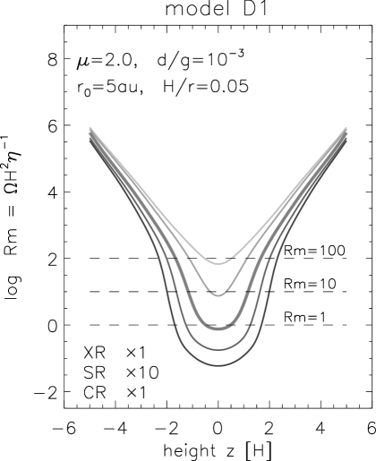
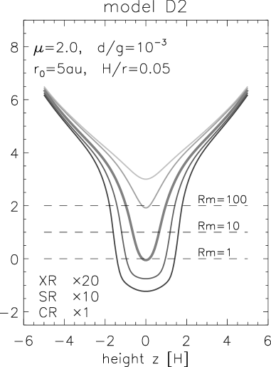
Figure 1: Vertical $\eta$ profiles for runs D1 and D2, in terms of the magnetic Reynolds number, $\mathrm{Rm}=\Omega\,H^{2}\,\eta(z)^{-1}$, as given by our ionisation model. The thick line corresponds to the adopted initial model (with $\Sigma=135\,\rm g\,\rm cm^{-2}$). Thin lines on either side are for disc masses increased and reduced by factors of two, and demonstrate the strong dependence on the mass column. A dead zone is expected for $\mathrm{Rm}\,\hbox{\lower 1.50696pt\hbox{$\sim$}\hbox to0.0pt{\hss\raise 1.50696pt\hbox{$<$}}}\,10$ (cf. Turner & Sano, 2008).

Because the numerically allowed diffusive time step decreases with the grid spacing squared, adequately resolved dynamical simulations can become prohibitive in the presence of high diffusion coefficients. Given limited computational resources, we therefore decided to confine the dynamical span in the magnetic diffusivity $\eta$ to a reasonable range. We primarily do this by including an ambient ionisation due to the decay of short-lived radionuclides (SR), which we further enhance by a factor of ten compared to the fiducial value of $\zeta_{\rm SR}=3.7\!\times\!10^{-19}\,\rm s^{-1}$ given in Turner & Drake (2009). As can be seen in Fig. 1, where we plot the resulting $\eta$ profiles, the floor in the magnetic Reynolds number due to the ambient level of ionisation is well below the expected threshold for the formation of a dead zone. This implies that we should not expect our results to be significantly affected by enhancing the effects of decaying radionuclides.

We remark that, compared to previous work, our diffusivity profiles overall imply lower magnetic Reynolds numbers. Given that Fleming et al. (2000) have found a critical $\mathrm{Rm}_{\rm c}\simeq 10^{4}$ for sustained MRI in a zero-net-flux configuration, we expect that the amplitude of an external net-flux will have a significant impact on the level of turbulence.

2.3.2 Sub-cycling

Notwithstanding the moderate range in $\eta$, the numerical constraint given by the diffusive propagation of information is one of the main limiting factors in our simulations. To avoid a degradation of the numerical accuracy in the MRI-active region by an excessively low numerical time step in the dead zone, we choose to account for the two separate regimes in $\mathrm{Rm}$. This is done by operator-splitting the diffusive term in the induction equation and applying a sub cycling-scheme for its update. By doing so, we are able to integrate the non-diffusive part of the MHD equations with a longer time step, enhancing the accuracy of the solution in regions of low magnetic diffusivity.

2.4 Code improvements

Properly resolving the growing modes of the magneto-rotational instability (MRI) with Godunov-type codes has been found to depend on the reconstruction strategy used and on the ability of the Riemann solver to capture the Alfvénic mode (Balsara & Meyer, 2010). To improve the representation of discontinuities in our finite volume scheme, we recently extended the nirvana-iii code with the Harten–Lax–van Leer Discontinuities (HLLD) approximate Riemann solver introduced by Miyoshi & Kusano (2005). To guarantee the required directional biasing of the electromotive force interpolation (cf. Flock et al., 2010), we have implemented and tested the upwind reconstruction procedure of Gardiner & Stone (2005).

To enhance the stability of our code in the strongly magnetised corona, we gradually degrade the reconstruction order from second- to first-order accuracy near the vertical domain boundaries, thus avoiding undershoots in the hydrodynamic state variables in strong shocks.

2.4.1 Artificial mass diffusion

To facilitate the study of a low-beta disc corona, Miller & Stone (2000) have introduced the concept of a so-called Alfvén speed limiter, circumventing prohibitively high signal speeds in low-density regions. Such a limiter can in principle be adopted for the approximate Riemann solvers we use. We chose, however, a different approach and instead add an artificial mass diffusion term to the equations of mass and momentum conservation. The diffusion coefficient is chosen to lie well below the truncation error in the bulk of the domain. In grid cells where the density contrast exceeds a specified dynamic range, $C_{\rm dyn}$, the coefficient is gradually adjusted according to

$$D(\rho)=\frac{1}{6}\ \left[1+\left(10^{C_{\rm dyn}}\,\frac{\rho}{\rho_{0}}\right)^{4}\right]^{-1/4}$$ (3)

such that the grid Reynolds number approaches order unity – coinciding with the stability limit for the explicit time integration of the diffusive term. The transition function is chosen in a way that the inverse operation can be efficiently implemented by means of consecutive square-root operations. We typically chose $C_{\rm dyn}=5$, resulting in four to five orders of magnitude in density contrast. We note that, because the diffusive fluxes are part of the finite volume update, this approach does not violate mass conservation, and therefore avoids the problems of enforcing an artificial floor value in the density. In conclusion, our approach has proven to greatly benefit the overall robustness without noticeably affecting the solution in the interior of the domain. Similarly to the limiters used by Miller & Stone (2000) and Johansen & Levin (2008), the Courant-Friedrichs-Lewy time-step constraint due to the fast magnetosonic mode is significantly alleviated, allowing for economical use of computing resources.

3 Disc model properties

	orbits	$\left<\right.\!\alpha\!\left.\right>$	$\sigma_{\Gamma}\ \ [\,\rm cm^{2}\,\rm s^{\!-2}]$	$\tau_{\rm c}\ \ [2\pi\Omega^{-1}]$	$C_{\sigma}(\Delta x)\ \ [H]$	$C_{\sigma}(e)\ \ [H/r]$
A1	217	0.0105	0.45$\,\times 10^{8}$	0.30	5.21$\,\times 10^{-3}$	2.68$\,\times 10^{-3}$
D1	224	0.0038	0.06$\,\times 10^{8}$	0.29	4.72$\,\times 10^{-4}$	1.54$\,\times 10^{-4}$
D2	223	0.0051	0.13$\,\times 10^{8}$	0.27	7.25$\,\times 10^{-4}$	2.50$\,\times 10^{-4}$
B1∗	505	$0.05\quad$	0.74$\,\times 10^{8}$	0.32	7.70$\,\times 10^{-3}$	2.77$\,\times 10^{-3}$

^∗torque corrected for 2D/3D evaluation (cf. Fig. 8 in Nelson & Gressel, 2010).

Table 2: Overview of simulation results. Gravitational torques $\Gamma$ represent the standard deviation $\sigma$ of a normal distribution (see Fig. 8), Coherence times $\tau_{\rm c}$ are from a fit to the torque ACF (see Fig. 9). The random walk amplitudes $C_{\sigma}(\Delta x)$ and $C_{\sigma}(e)$ refer to the dispersion in the displacement and eccentricity of a swarm of particles.

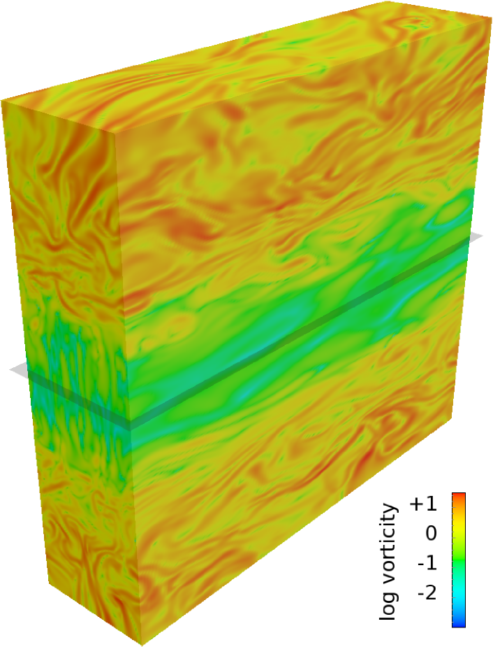
Figure 2: Visualisation of the turbulent flow structure. The colour coding indicates the vorticity, $\log_{10}\ |\nabla\times\mathbf{u}|$ of the perturbed flow $\mathbf{u}=\mathbf{v}-q\Omega x\hat{{\mathbf{y}}}$. While the turbulent regions above and below the dead zone show strongly folded vortex structures, the flow pattern near the midplane is dominated by shearing waves. The contrast in the vorticity amplitude is $\sim 100$.

In the following, we will present results from three different simulations (see Tab. 1 for details). To be able to make a quantitative comparison with respect to the effects of a dead zone, we performed a fiducial stratified model with fully active MRI, referred to as model A1. In general, this model agrees well with the unstratified simulations presented in paper I. For our standard dead zone model, D1, we choose the reference ionisation rates of Turner & Drake (2009) along with a dust-to-gas mass ratio of 1$\,:\,$1000, i.e., accounting for a modest depletion of the smallest grains by coagulation and sedimentation. The resulting diffusivity profile is plotted in the left panel of Figure 1.

The resulting dead zone in this model covers roughly $\pm 2H$, making it a reasonable proxy for what a realistic dead zone at $5\,\rm au$ might look like. Gaseous nebulae around newly forming stars, however, are subject to substantial variations in X-ray irradiation (Garmire et al., 2000), so for our second dead zone model, D2, we increase the stellar flux by a factor of twenty. We find the average total thickness of the dead zone to be reduced by roughly $1.5$ pressure scale heights in this case (see Fig. 1, right panel).

3.1 Hydromagnetic turbulence

One important result of the early simulations of layered accretion discs by Fleming & Stone (2003) was that the dead zone, despite its name, retains a non-negligible level of Reynolds stresses, namely in the form of waves that are excited in the active layers. These residual motions can clearly be seen in Fig. 2, where we have visualised the flow structure in terms of the logarithmic vorticity. The colour coding exhibits very distinct patterns in the two regions: while the MRI active layers show folded vortex features characteristic of developed turbulence, the dead zone region is clearly non-turbulent, and dominated by sheared density waves with $k_{R}\gg k_{\phi}$. At the interface between the two zones, one can furthermore see structures indicating some level of turbulent mixing into the dead zone. Because our model assumes that recombination on the surface of small dust grains is efficient (leading to a recombination time scale much smaller than the dynamical mixing time scale) this does not, however, have an effect on the extent of the dead zone.

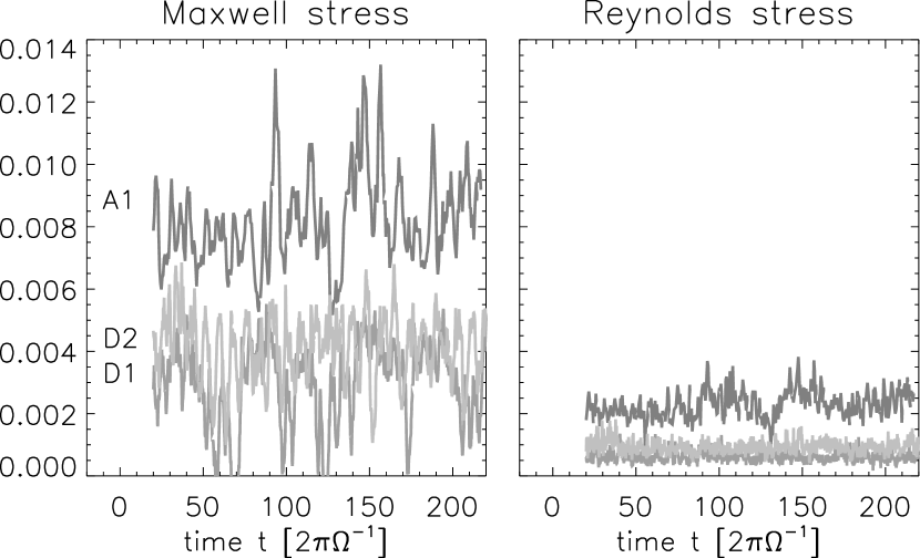
Figure 3: Comparison between the box averaged turbulent Maxwell- and Reynolds stresses. Values are normalised by the gas pressure in the disc midplane, $p_{0}$. The time-averaged sums of these, i.e., the $\alpha$ parameters, are listed in column three of Tab. 2.

Our primary aim in this paper is to examine statistically the dynamical evolution of planetesimals embedded in turbulent discs with and without dead zones. In order to do this we require a quasi-stationary model of turbulence. As can be seen in Fig. 3, where we plot the time variation of the box-averaged transport coefficients, our models fulfil this requirement of a stationary mean with (admittedly strong) superposed fluctuations. Because the bulk of the transport is associated with the MRI-active regions, the turbulent stresses only seem to depend weakly on the actual width of the dead zone. We remark that due to the different field configuration, the overall strength of the turbulence is somewhat weaker than in our previous non-stratified models presented in paper I. This is related to buoyant loss of magnetic flux from the disc in stratified simulations, and is consistent with recent results in the literature (cf. Davis et al., 2010, and references therein).

Figure 4: Spatio-temporal evolution of (a) mean toroidal field, (b) total Maxwell stress, for the fully active model A1.

3.2 Spatio-temporal disc evolution

Figure 4 shows space-time plots of the mean toroidal magnetic field $\bar{B}_{y}(z,t)$, as well as the total Maxwell stress for the fully active model A1. Probably the most striking features in this plot are the periodic “butterfly” patterns in the large-scale magnetic field, which are commonly observed in this type of simulation (e.g. Davis et al., 2010; Flaig et al., 2010). Because the upwelling field structures are not associated with a bulk motion of the flow, the likely explanation for the emerging patterns is a mean-field dynamo as recently re-investigated by Gressel (2010). Even though we see quite strong fluctuations in the total Maxwell stress, the overall state is quasi stationary. Note that the two most prominent peaks of the total Maxwell stress (i.e. around 140-145 and 155-160 orbits) are (a) due to a strong mean field, and (b) confined to one half of the box. The situation of magnetic activity being dominant in one half of the disc has been observed before (see e.g. fig. 7 in Miller & Stone, 2000), and might be explained by equally strong quadrupolar and dipolar contributions. These cancel on one side and, at the same time, add-up on the opposite side, resulting in the observed lopsided appearance. In fact, we cannot define a clear parity of the field in Fig. 4, which implies that the dipolar and quadrupolar dynamo modes seem to possess similar growth rates.

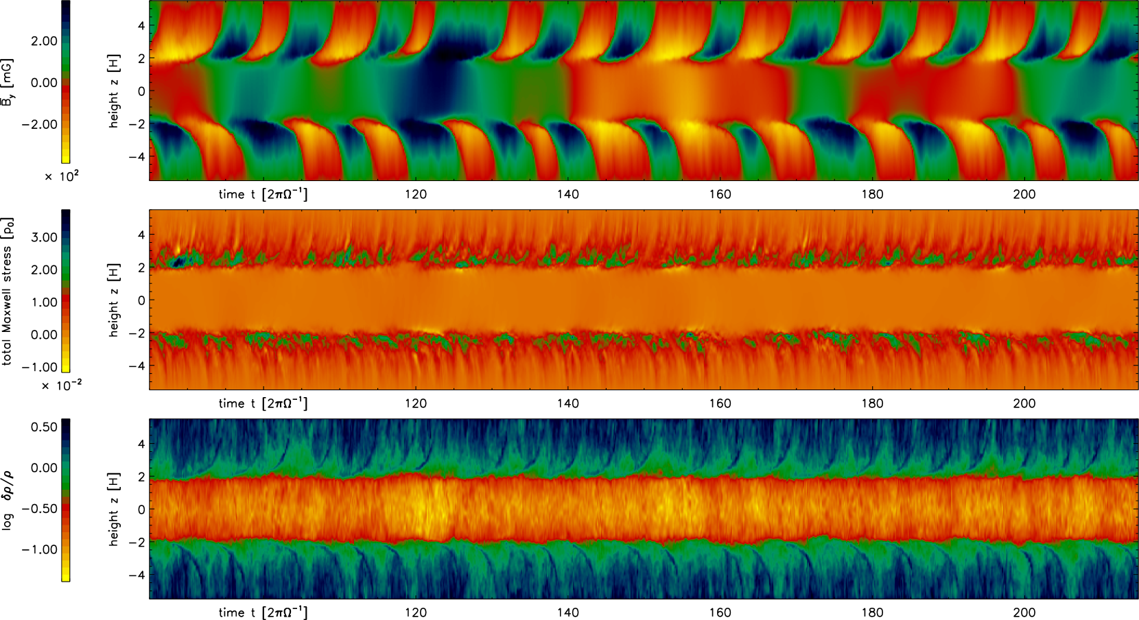
Figure 5: Same as Fig. 4, but for the dead zone model D1, and including an extra panel showing the relative density fluctuations (logarithmic). The horizontal field exhibits the same dynamo cycles in the MRI active layers. As already seen by Turner & Sano (2008), the toroidal field leaks into the diffusively dominated midplane region, contributing to the stresses. Despite the absence of strong turbulent fields, density fluctuations reach a level of 10-20% within the dead zone.

In the following discussion, we will focus on the vertical structure of the disc and how it is shaped by the presence of a dead zone. For this we will show the time-averaged vertical profiles of various quantities. To demonstrate that this is a meaningful procedure, we provide space-time diagrams of three representative quantities (Fig. 5) for model D1. Again, the mean toroidal field generally is of irregular parity, i.e., neither quadrupolar nor dipolar symmetry is seen to prevail. Whether the concept of a global parity is relevant in the presence of a highly diffusive “insulating” layer remains a matter of discussion. It is interesting to note, however, that MRI channel modes – which are a non-linear solution to local net-flux MRI simulations – represent global modes even when stratification is included (Latter et al., 2010). In fact, we see some indication of channels in our simulations, most prominently in the density (compare the lower panel in Fig. 5 with Latter et al., 2010, fig. 3).

Quite remarkably, the number of field reversals related to the dynamo-cycle seems to be largely unaffected by the presence of the dead zone. As mentioned above, one main motivation in explaining the rising patterns by a mean-field dynamo, was the absence of a bulk motion near the midplane – implying that the pattern speed cannot be explained by the Parker instability (Shi et al., 2010). The key in explaining the upward motion was a negative buoyant $\alpha$ effect near the midplane (Rüdiger & Pipin, 2000; Brandenburg, 2008). With the pattern in the disc halo being unchanged in the presence of a dead zone, this picture possibly has to be amended. Naively, for a positive $\alpha$ effect in the halo (as found by Gressel, 2010), one would not expect an outward butterfly diagram from classical theory – demonstrating the need for non-linear feedback both in the diagnostics (Rheinhardt & Brandenburg, 2010) as well as in the modelling (Brandenburg, Candelaresi & Chatterjee, 2009; Courvoisier, Hughes & Proctor, 2010).

We note however, that because of the presence of the weak net vertical flux in our current simulations, they are not strictly comparable to our previous work. Due to the net flux, a possible explanation of the unchanged migration direction might be the presence of prevailing channel modes. These were shown to produce a strong negative helicity (cf. fig. 4 in Gressel, 2010), compatible with the upward motion of the wave patterns.

Now focusing our attention to the actual dead zone region, we see that a significant amount of azimuthal (and in fact, radial) field diffuses in to the low-$\mathrm{Rm}$ region around the midplane. This leakage has first been seen in simulations by Turner et al. (2007) and Turner & Sano (2008), which are very similar to ours and also contain a weak net vertical field. In contrast to this, the simulations by Fleming & Stone (2003), Oishi, Mac Low & Menou (2007) and Ilgner & Nelson (2008), which apply a zero-net-flux configuration, do not show such an effect. It seems peculiar, however, that the presence of a net flux should play a role in this context. As Ilgner & Nelson (2008) illustrate in their fig. 2, the assumed diffusivity profiles of Fleming & Stone (2003) result in moderately high magnetic Reynolds numbers near the midplane. On the contrary, in the model of Turner, Sano & Dziourkevitch (2007) and also in our model (cf. Fig 1) the magnetic Reynolds number reaches much lower values of $\mathrm{Rm}<10$ for $|z|<H$, leading to a much reduced diffusion time scale, possibly facilitating the leakage of large-scale field from the disc halo into the dead zone.

Finally, we note that relative density fluctuations remain at a level of up to ten per cent within the dead zone – as seen in the lowermost panel of Fig. 5. Episodes of lower perturbance (as indicated by lighter colours) are clearly correlated with strong azimuthal field, and notably with a negative Maxwell stress at the interface between the dead and active zones. As already mentioned above, we see indications of persistent channel modes (dark streaks above $|z|\,\hbox{\lower 1.50696pt\hbox{$\sim$}\hbox to0.0pt{\hss\raise 1.50696pt\hbox{$>$}}}\,2H$), which are not unexpected given the magnetic configuration. It might be argued that such features are overly pronounced at the current numerical resolution, and might be destroyed by parasitic instabilities (Pessah & Goodman, 2009; Latter et al., 2009, 2010) when the resolution is further increased.

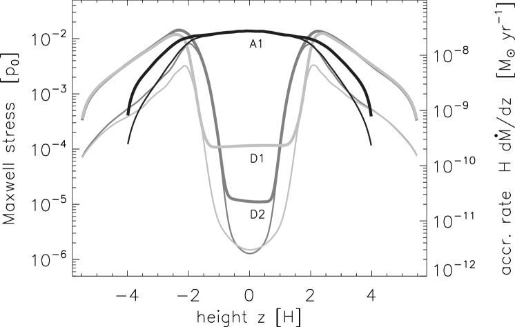
Figure 6: Maxwell stresses for the different models. Thick lines indicate the total stress $\propto-\left<\right.\!B_{R}\,B_{\phi}\!\left.\right>$, thin lines represent the turbulent contribution $\propto-\left<\right.\!B^{\prime}_{R}\,B^{\prime}_{\phi}\!\left.\right>$, where $B^{\prime}\!=\!B-\left<\right.\!B\!\left.\right>$. The vertically integrated mass accretion rates (see rhs axis) for the models D2, D1 and A1, are $9.85\times 10^{-8}$, $7.82\times 10^{-8}$, and $1.36\times 10^{-7}\,\rm M_{\odot}\,\rm yr^{-1}$, respectively. Note the unexpected trend in the depth between models D1 and D2, as opposed to Fig. 7.

3.3 Disc vertical structure

Figure 6 shows time-averaged vertical profiles of the $R\phi$ components of the Maxwell stress tensor. Because we use an isothermal equation of state, resulting in a constant sound speed, $c_{\rm s}$, these profiles translate directly into a fractional mass accretion rate as indicated by the right-hand axis. The values on this axis are given by the expression $H\,{\rm d}\dot{M}/{\rm d}z=3\pi\,c_{s}\,H^{2}\,\rho(z)T_{r\phi}/p(z)$, which can be derived from the usual approximation for the mass accretion rate in a steady disc $\dot{M}=3\pi\nu\Sigma$, but relaxing the assumption that the effective viscous stresses are independent of $z$.

The vertically integrated mass flow rates generated by the magnetic stresses are $9.85\times 10^{-8}$ and $7.82\times 10^{-8}\,\rm M_{\odot}\,\rm yr^{-1}$ for runs D2 and D1, respectively. This similarity is expected because the heights of the dead and active zones about the midplane in each model are similar ($\sim 1.5H$ and $2H$, respectively, for the dead zones in models D2 and D1). The mass flow rate in the fully active run A1 is $1.36\times 10^{-7}\,\rm M_{\odot}\,\rm yr^{-1}$, nearly twice that observed in the model with the largest dead zone. Given that the bulk of the mass in the disc lies within the dead zone, where the Maxwell stresses for models D2 and D1 are factors of $\sim 10^{-2}$ and $10^{-3}$ smaller than for model A1, the bulk of the transport in models D1 and D2 happens in the active layers because the stresses (and effective viscosity coefficient $\alpha$) remain large there.

Figure 6 shows that the Maxwell stresses in the midplane regions are dominated by large-scale fields in runs D1 and D2 – even more so than in the halo regions of the fully active run A1. This result agrees broadly with recent simulations (cf. fig. 4 in Turner & Sano, 2008) which included similar physical effects. While the turbulent contribution to the Maxwell stress (thin lines) falls-off to $\simeq 10^{-6}$ in the dead zone for both models D1 and D2, one can clearly see that the effect of the greater dead zone width in model D1 is compensated for by a shallower valley in the total Maxwell stress (thick lines). The inverse top-hat shape of the profiles is likely related to large-scale field diffusing into regions of intermediate $\mathrm{Rm}$, as seen in the topmost panel of Figure 5. Given that the transition region is closer to the low-$\beta$ halo for model D1 (with a wider dead zone), it seems plausible that the strength of the regular field is larger in this case. Clearly, the contribution due to the fluctuating fields becomes negligible in both cases.

Considering that, for model D1, the floor value of the Maxwell stress is of the same magnitude as the Reynolds stress (cf. Fig. 7), such large-scale stresses might play an important role in mediating mass transport within the dead zone – making a more detailed future study of the discussed trend worthwhile, particularly in the context of global disc models, where it may be possible to observe large scale accretion flows in dead zones.

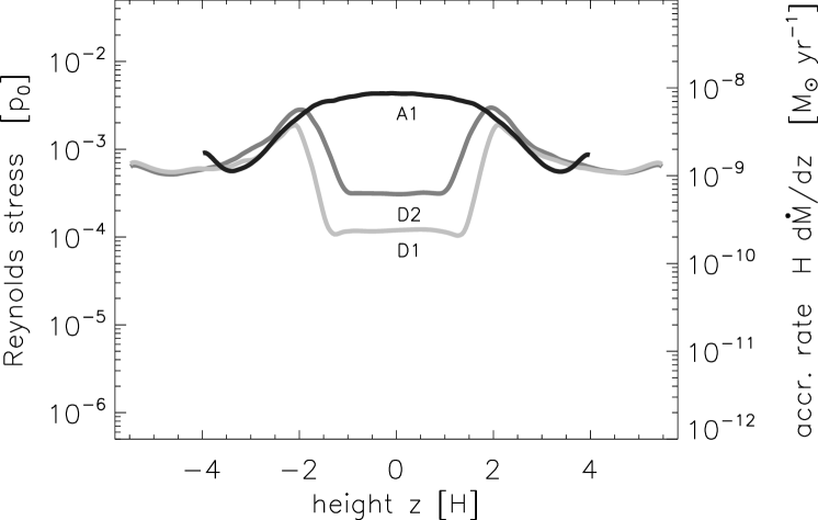
Figure 7: Same as Fig. 6, but for the Reynolds stress $\left<\right.\!\rho\,v_{R}\delta v_{\phi}\!\left.\right>$. The vertically-integrated mass accretion rates are $2.08\times 10^{-8}$, $1.39\times 10^{-8}$, and $3.64\times 10^{-8}\,\rm M_{\odot}\,\rm yr^{-1}$ for models D2, D1, and A1, respectively.

In Figure 7, we plot vertical profiles of the time-averaged Reynolds stress. As expected, the lines agree very well in the MRI-active regions. Comparing the models D1 and D2, we now see a correspondence between the dead zone width and depth, as expected. It appears that larger and more massive active zones lying above and below the dead zone are more able to excite higher amplitude sound waves which are able to propagate into the dead zone, generating a correspondingly larger Reynolds stress there.

Based on two runs with different (zero net flux) field topologies, Fleming & Stone (2003) concluded that “the Reynolds stress in the midplane does not seem to depend on the size of the dead zone but rather the amplitude of the turbulence in the active layers”. This is clearly not the case for our models D1 and D2, which show quite different Reynolds stresses in the dead zone, while having almost identical levels of Maxwell stresses – both in the total and fluctuating part – within the active region (see Figs. 6 and 7, respectively). While we reckon that the larger Reynolds stress is related to the larger mass of the active layer in model D2, this discrepancy may also be due to the presence of large-scale fields diffusing into the midplane region in our simulations. Note that Fleming & Stone (2003) did not mention such fields in their discussion.

4 Characterising the gravitational forcing

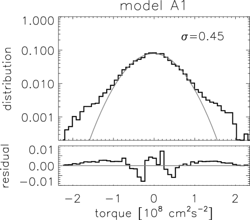
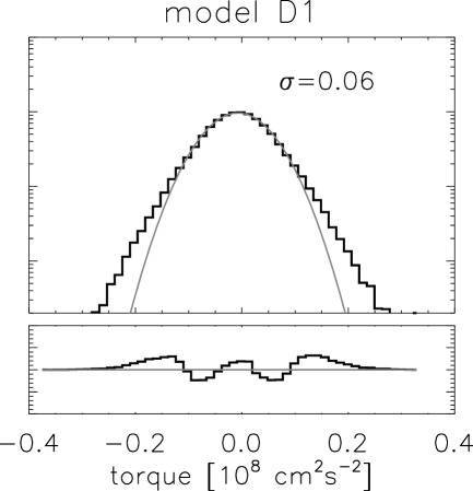
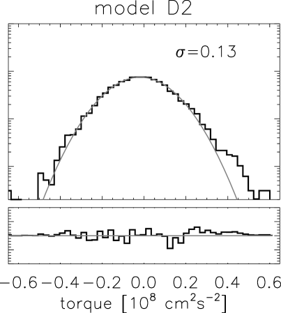
Figure 8: Torque histograms for models A1, D1 and D2. The grey lines indicate fitted normal distributions, for which standard deviations are given (note the different scale on the abscissae). While the torques within the dead zone are well approximated by a Gaussian, the distribution in model A1 develops some deviations for large torques.

As first suggested by the global simulations of Nelson (2005), the stochastic gravitational forces associated with density fluctuations from developed MRI turbulence have the potential to limit severely the growth of planetesimals. In paper I, we have confirmed this original finding in the framework of global simulations and local simulations with large enough box sizes, but in which the vertical component of gravity was neglected. In the following section, we extend this work to the case of stratified discs with and without a dead zone. To facilitate a direct comparison, we here focus on the case of a moderately strong net vertical field. In this respect, the results should be interpreted as upper limits. To obtain lower limits for the torque amplitude, models with nominal dead zones and applying a zero-net-flux configuration will be required.

4.1 Stochastic torques

Figure 8 shows distribution functions of gravitational torques along the $y$-direction in our simulation box. The histograms are computed from the time series of a set of 25 particles in each simulation run. Unlike Oishi et al. (2007), we do not observe transients in the time series, and the torques are indeed quasi-stationary in the interval [20,210] orbits, which has been used to obtain each histogram. As required for a simplified treatment in terms of a stochastic Monte Carlo model, the histograms are well represented by a normal distribution. Notably, there are moderate power-law tails in the fully active run A1, indicating some level of non-Gaussian fluctuations (also cf. fig. 7 in paper I). The amplitude of the torques in the different runs roughly scales with the square-root of the midplane Reynolds stress. This arises because the density fluctuations scale linearly with the velocity fluctuations, and coincides with the scaling found in section 3.3 of Baruteau & Lin (2010).

Apart from the torque amplitude, the ability to stochastically amplify particle motions depends on the degree of coherence in the fluid patterns. Building on our work from paper I, we here apply the same formalism and study temporal torque autocorrelation functions (ACFs). We use the fitting formula introduced in section 3.3 of paper I, i.e.

$$S_{\Gamma}(\tau)=\left[(1-a)+a\,\cos(2\pi\,\omega\,\tau)\right]\,{\rm e}^{-\tau/\tau_{\rm c}}\,,$$ (4)

with free parameters, $a$, $\omega$, and $\tau_{\rm c}$. As discussed in paper I, we assume two components to better fit the shape of the ACF: (i) an exponential decay representing the truly stochastic part of the torque time series; (ii) a modulation due to “wavelike” behaviour, i.e., a negative dip in the ACF reflecting the fact that density enhancements swashing over the region of influence will produce torques of opposite signs when approaching and receding the test particle. Such a feature is also seen in the corresponding Figs. 9 and 15 of Oishi et al. (2007) and Yang et al. (2009), respectively, complicating the interpretation of the results.

In paper I, we have discovered certain trends in the amplitude of the latter effect, which are probably related to the finite size of the computational domain. Because the periodic box in some respect acts as a resonator, the wavelike component probably appears too pronounced in local simulations. This demonstrates that one does well keeping in mind the limitations of local boxes in terms of the allowed dynamics (also see Regev & Umurhan, 2008). The parameter of interest, of course, is the correlation time $\tau_{\rm c}$ of the stochastic perturbation. While waves represent ordered motion, it is this stochastic part that ultimately produces the random-walk amplification of the particle motions.

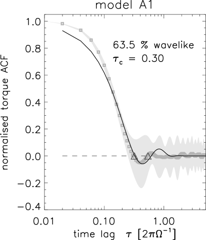
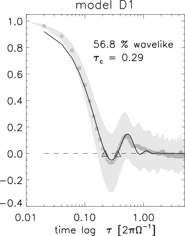
Figure 9: Torque autocorrelation function (ACF) for models A1 and D1. The black lines indicate model fits (see text), showing that motions are coherent over approximately one third of the orbital time scale. The ACF for model D2 is very similar to D1 and is hence not shown.

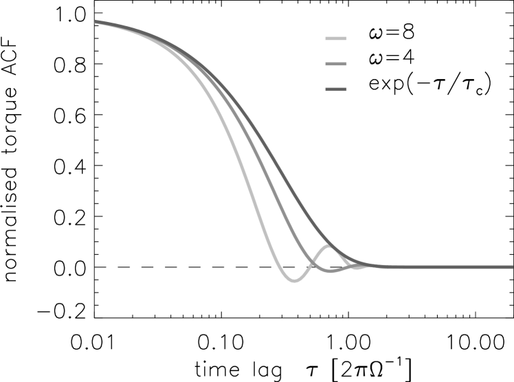
Figure 10: Comparison of three different model ACFs as given by Eqn. (4). All curves have the same coherence time $\tau_{\rm c}=0.3$ and yet show quite different zero-crossings.

In the following, we rely on the approach taken in Eqn. (4) providing an effective deconvolution of the two effects. The resulting fits for models A1 and D1 are shown in Fig. 9. Unlike model B1 (cf. fig. 9 in paper I), model A1 shows a moderate level of modulation. Given the horizontal box dimensions of $4\!\times\!16H$, this is somewhat unexpected as we observed a consistent trend towards weaker modulation for larger box sizes in paper I. This being said, the fitted coherence time of $\tau_{\rm c}=0.30$ in model A1 is in striking agreement with our earlier unstratified model. The torque ACF of the dead zone model D1 shows a comparable amplitude in the modulation and has an almost identical value of $\tau_{\rm c}=0.29$.

With respect to the artificial forcing function used in the 2D global simulations of Baruteau & Lin (2010), we note that our value for $\tau_{\rm c}=0.3$ coincides with the one stated for their “reduced lifetime” case. Comparing our ACF with the one in their Fig. 2, there appears, however, to be a discrepancy of a factor of two in the first zero crossing. This can possibly be explained by a different modulation of the exponential decay as exemplified in Figure 10. All curves have a common $\tau_{\rm c}=0.3$. Moreover, the first two curves have a 60% wavelike modulations with frequency $\omega$ as indicated, while the third is a simple exponential. Owing to the confusion with respect to the definition of the coherence time, it seems worthwhile to further study how the spectrum of modes affects the apparent coherence. Nevertheless, given the actual type of forcing used in Baruteau & Lin (2010), i.e. a spectrum of wavelike motions, one may be surprised how similar the ACFs indeed look. Going back to Fig. 2, it however becomes obvious that it is not the turbulence we need to approximate but only the spiral density waves with uncorrelated phases that it creates.

The corresponding ACF for model D2 is omitted here, as it is very similar to D1. The fitted coherence time for model D2 is $\tau_{\rm c}=0.27$, in good agreement with the other two runs. We therefore conclude that the presence (and depth) of a dead zone does have little influence on the temporal torque statistics and merely affects the amplitude of the stirring process.

Model	size	$v_{\rm disp}$ [$\,\rm m\,s^{-1}\,$]	$v_{\rm disp}$ [$\,\rm m\,s^{-1}\,$]	$v_{\rm crit}$ [$\,\rm m\,s^{-1}\,$]	$v_{\rm crit}$ [$\,\rm m\,s^{-1}\,$]	$v_{\rm crit}$ [$\,\rm m\,s^{-1}\,$]	$t_{\rm eq}$ [$\,\rm yr\,$]
		(gas drag)	(collisional)	(weak)	(strong)	(rubble pile)
A1	$100\,\rm m$	73.8	79.9	1.0	7.7	-	$1.91\!\times\!10^{4}$
	$1\,\rm km$	159.0	251.4	2.9	15.2	-	$8.85\!\times\!10^{4}$
	$10\,\rm km$	342.8	795.0	26.3	137.0	58.5	$4.11\!\times\!10^{5}$
	$100\,\rm km$	738.2	2514.3	262.6	1368.0	585.4	$1.91\!\times\!10^{6}$
D1	$100\,\rm m$	11.0	4.5	1.0	7.7	-	$2.20\!\times\!10^{4}$
	$1\,\rm km$	23.7	14.3	2.9	15.2	-	$2.20\!\times\!10^{5}$
	$10\,\rm km$	51.0	45.4	26.3	137.0	58.5	$2.21\!\times\!10^{6}$
	$100\,\rm km$	110.0	143.5	262.6	1368.0	585.4	$10.3\!\times\!10^{6}$
D2	$100\,\rm m$	15.2	7.4	1.0	7.7	-	$2.22\!\times\!10^{4}$
	$1\,\rm km$	32.7	23.3	2.9	15.2	-	$2.21\!\times\!10^{5}$
	$10\,\rm km$	70.5	73.9	26.3	137.0	58.5	$1.60\!\times\!10^{6}$
	$100\,\rm km$	153.4	233.6	262.6	1368.0	585.4	$7.58\!\times\!10^{6}$

Table 3: Results for the equilibrium velocity dispersions obtained for each model as a function of the planetesimal sizes, and as a function of the damping mechanism. Also tabulated is the time required to grow to the smaller of the equilibrium velocity dispersion values given for each model each size.

5 Eccentricity stirring and planetesimal accretion

To study the excitation of the velocity dispersion and the radial diffusion of embedded boulders, planetesimals, and protoplanets, in each run we integrated the trajectories of a swarm of 25 non-interacting test particles subject to perturbations from the gravitational potential of the gas disc. Unlike in paper I, we here focus on larger bodies and neglect the effects of aerodynamic interaction. This is warranted for solids with radii above $\simeq 100\,\rm m$ (cf. paper I where the results for planetesimals with sizes in the range $100\,\rm m$ - $10\,\rm km$ were found to be similar for run times on the order of a few hundred planetesimal orbits). The upper limit for the size range considered here is given by the constraint that perturbations of the disc remain weak such that spiral wave excitation and gap-opening can be ignored. This is the case for planetesimals and small protoplanets, where feedback onto the disc can be ignored.

Although we do not consider in detail the dynamics of metre-sized boulders that are strongly coupled to the gas via drag forces in this paper, we recall from paper I that such bodies quickly achieve random velocities very similar to the turbulent velocity field of the gas. The midplane r.m.s. turbulent velocity for the fully turbulent model A1 is found to be $v_{\rm turb}=(76.6\pm 6.5)\,\rm m\,s^{-1}$, and for model D1 $v_{\rm turb}=(17.8\pm 2.6)\,\rm m\,s^{-1}$. For model D2 $v_{\rm turb}=(28.5\pm 3.6)\,\rm m\,s^{-1}$.

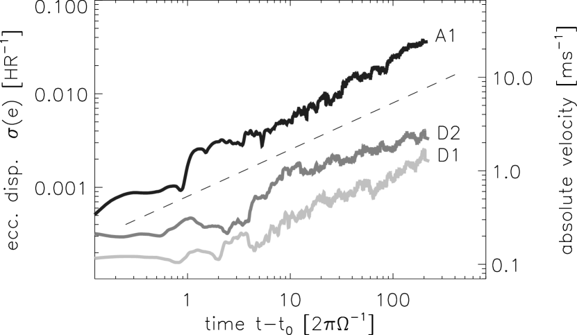
Figure 11: Random-walk eccentricity growth for the dispersion, $\sigma(e)$, of sets of 25 particles in each run. The expected $\sqrt{t}$ behaviour is indicated by the dashed line. The rhs axis gives the corresponding radial velocity dispersion, leading to disruptive relative velocities for the fully active run A1. The amplitudes for the dead zone runs are lower by a factor of 10-20.

We now consider the dynamics of larger planetesimals. The excitation of the eccentricity (and equivalently the radial velocity dispersion) can be seen in Fig. 11, where we plot the r.m.s. values of these quantities averaged over the planetesimal swarms as a function of time for the runs A1, D1 and D2. The time history is consistent with a random-walk behaviour, indicated by the dashed line representing an $e(t)\sim\sqrt{t}$ dependence. Expressing the time evolution of the eccentricity according to

$$e(t)/h=C_{\sigma}(e)\sqrt{t},$$ (5)

where $h=H/r$, and the time is measured in local orbits, we obtain the following values for the amplitude factors, $C_{\sigma}(e)$ (which are also listed in Tab. 2): $2.68\times 10^{-3}$, $2.50\times 10^{-4}$, and $1.54\times 10^{-4}$ for models A1, D2, and D1 respectively. Despite the different levels of turbulence (as reflected in both $\alpha$ and $\Gamma$), the values in Tab. 2 show that the stirring amplitude of model A1 agrees quite well with the unstratified model from paper I. The amplitudes from the dead zone runs D2 and D1 are lower by a factor of $\simeq 11$ and $\simeq 17$, respectively, showing that the presence of the dead zone has a clear and measurable effect on the strength of eccentricity stirring.

5.1 Long-term evolution

As we have only been able to run our simulations for about 200 orbits, it is important to consider the long term evolution by examining the magnitude of the equilibrium eccentricity that is expected to arise through the balance between turbulent eccentricity excitation and gas drag and/or collisional damping (Ida et al., 2008). The question of whether or not collisional growth of planetesimals may occur in the different disc models is determined by the velocity dispersions obtained relative to the disruption/erosion velocity thresholds, and this point is addressed in the discussion that follows.

5.1.1 Gas drag damping

We have not included gas drag or collisional damping in the simulations presented in this paper, but gas drag was included in the runs presented in paper I, and they showed that over run times of a few hundred orbits the gas drag has little influence on the eccentricity for planetesimals with radii $R_{p}\geq 100\,\rm m$. We adopt the usual expression for the gas drag force (Weidenschilling, 1977)

$${\bf F}_{\rm drag}=\frac{1}{2}C_{\rm D}\pi R_{\rm p}^{2}\rho\ |{\bf v}_{\rm p}-{\bf v}_{\rm g}|\ ({\bf v}_{\rm p}-{\bf v}_{\rm g})$$ (6)

where $C_{\rm D}$ is the drag coefficient. For making simple estimates we take the value $C_{\rm D}=0.44$, appropriate for larger planetesimals for which the Reynolds number of the flow around the body ${\cal R}_{e}>800$. The eccentricity growth over time is given by (5) where the time, $t$, is measured in local orbits. Following the same procedure adopted in paper I, and calculating the equilibrium velocity dispersion by equating the eccentricity growth time scale and the gas drag-induced damping time scale, we obtain

$$v_{\rm disp}=\left(\frac{4C_{\sigma}^{2}(e)h^{2}R_{\rm p}\rho_{\rm p}v^{2}_{\rm k}}{10^{9}C_{\rm D}\rho}\right)^{1/3}$$ (7)

where $R_{\rm p}$ and $\rho_{\rm p}$ are the planetesimal radius and density, and $v_{\rm k}$ is the Keplerian velocity. Note that the form taken by (7) now assumes that the system evolution time given in (5) is expressed in seconds. The equilibrium velocity dispersions obtained using (7) for each disc model and planetesimal size are listed in the third column of Tab. 3.

5.1.2 Collisional damping

The effects of collisional damping, due to inelastic collisions between planetesimals, may be estimated by noting that the collisional damping time scale is given by the product of the collision time scale and the number of collisions required to damp out the kinetic energy of random motion for a typical planetesimal. This approach is similar to that adopted by Ida et al. (2008). The collision time (neglecting the effect of gravitational focusing) is given by

$$t_{\rm coll}=\frac{1}{n_{\rm p}\pi R_{\rm p}^{2}v_{\rm disp}},$$ (8)

where $n_{\rm p}$ is the number density of planetesimals. This may be approximated by $n_{\rm p}=\Sigma_{\rm p}/(2\,H_{\rm p}\,m_{\rm p})$, where $H_{\rm p}=v_{\rm disp}/\Omega_{k}$ and $\Sigma_{\rm p}$ is the mass surface density of planetesimals. The coefficient of restitution is given by $C_{\rm R}=v_{\rm f}/v_{\rm i}$, where $v_{\rm i}$ and $v_{\rm f}$ are the initial and final velocities associated with a collision. The number of collisions required to damp $v_{\rm disp}$ is therefore

$$N_{\rm coll}=\frac{1}{1-C_{\rm R}}\,.$$ (9)

Combining Equations (8) and (9) we obtain the collision damping time:

$$\tau_{\rm c-damp}=\frac{8R_{\rm p}\rho_{\rm p}}{3\Sigma_{\rm p}\Omega_{\rm k}}\left(\frac{1}{1-C_{\rm R}}\right)\,.$$ (10)

Equating the collisional damping time with the eccentricity growth time associated with (5) – and given explicitly by equation (16) in paper I – yields an expression for the equilibrium velocity dispersion

$$v_{\rm disp}=\sqrt{\frac{4R_{\rm p}\rho_{\rm p}C_{\sigma}^{2}(e)h^{2}v_{k}^{2}}{10^{9}\Sigma_{\rm p}\Omega_{k}}\left(\frac{1}{1-C_{\rm R}}\right)}\,.$$ (11)

The value to be adopted for the coefficient of restitution, $C_{\rm R}$, depends on the material composition, the impact velocity, and whether or not the planetesimals may be considered to be monolithic bodies or rubble piles held together by self-gravity alone. Adopting the velocity dependent formula from Bridges et al. (1984)

$$C_{\rm R}={\rm MIN}\,\left\{\ 0.34\left(\frac{v_{\rm disp}}{1\,{\rm cm\,s}^{-1}}\right)^{-0.234},\ 1\ \right\}\,,$$ (12)

we find that $C_{\rm R}\simeq 0$ for the values of the radial velocity dispersion, $v_{\rm disp}$, that we obtain in the simulations. We therefore adopt $C_{\rm R}=0$ when estimating the equilibrium $v_{\rm disp}$. The equilibrium velocity dispersions obtained using (11) for each disc model and planetesimal size are listed in the fourth column of Table 3. In obtaining these values we assume that $\Sigma_{\rm p}=4\times(\Sigma/250)$ – i.e. the surface density of solids is a factor of $1/250$ lower than the gas surface density, but is augmented by a factor of 4 beyond the ice-line. We further assume that all disc solids are incorporated within planetesimals of size $R_{\rm p}$ for each size that we consider.

5.1.3 Disruption velocity thresholds

The consequences of the equilibrium velocity dispersions obtained from equations (7) and (11) for planetary growth can only be determined by comparing them with the disruption/erosion thresholds for colliding bodies (Benz & Asphaug, 1999; Stewart & Leinhardt, 2009), and with the escape velocities associated with the planetesimals. In a recent study, Stewart & Leinhardt (2009) present a universal law for collision outcomes in the form

$$\frac{M_{\rm lr}}{M_{tot}}=1-\frac{1}{2}\frac{Q_{\rm R}}{Q_{\rm D}},$$ (13)

where $M_{\rm lr}$ is the mass of the largest post-collision remnant, $M_{\rm tot}$ is the total mass of the colliding objects $M_{1}+M_{2}$, and $Q_{\rm R}$ is the reduced mass kinetic energy normalised by the total mass

$$Q_{\rm R}=\frac{M_{1}M_{2}}{2M^{2}_{\rm tot}}V_{\rm I}^{2}.$$ (14)

Here $V_{\rm I}$ is the impact velocity. For accretion to occur during a collision between equal sized bodies, we require $M_{\rm lr}/M_{\rm tot}>1/2$, or equivalently $Q_{\rm R}/Q_{\rm D}<1$, such that $Q_{\rm D}$ is the collisional disruption or erosion threshold.

The value of $Q_{\rm D}$ is sensitive to factors that influence the energy and momentum coupling between colliding bodies (e.g. impact velocity, strength and porosity). Stewart & Leinhardt (2009) fit results from their numerical simulations and data in the literature using the expression

$$Q_{\rm D}=\left[q_{\rm s}R_{12}^{9\mu_{\rm m}/(3-2\phi_{\rm m})}+q_{\rm G}R_{12}^{3\mu_{\rm m}}\right]V_{\rm I}^{(2-3\mu_{\rm m})}\,,$$ (15)

where $q_{\rm s}$, $q_{\rm G}$, $\phi_{\rm m}$ and $\mu_{\rm m}$ are parameters. $R_{12}$ is the spherical radius of the combined mass, assuming $\rho_{\rm p}=1\,\rm g\,\rm cm^{-3}$. Since we use $\rho_{\rm p}=2\,\rm g\,\rm cm^{-3}$, and consider collisions between equal-sized bodies only, we have $R_{12}=2^{2/3}R_{\rm p}$. The first term on the right hand side of (15) represents the strength regime, while the second term represents the gravity regime. Small bodies are supported by material strength, which decreases as the planetesimal size increases. On the other hand, gravity increases in importance with growing planetesimal size – with the transition between the strength and gravity regimes occurring at $R_{\rm p}\approx 100\,\rm m$. Stewart & Leinhardt (2009) derive the following values for the above parameters for weak aggregates (weak rock): $q_{\rm s}=500$, $q_{\rm G}=10^{-4}$, $\mu_{\rm m}=0.4$, $\phi_{\rm m}=7$. For strong rocks they use basalt laboratory data and modelling results from Benz & Asphaug (1999) to obtain: $q_{\rm s}=7\times 10^{4}$, $q_{\rm G}=10^{-4}$, $\mu_{\rm m}=0.5$, $\phi_{\rm m}=8$. In the limit of large planetesimals, the disruption curve can be best fit by their results for colliding rubble piles, for which $Q_{\rm D}=1.7\times 10^{-6}R_{12}^{2}$. Given the uncertainties associated with the structure and material strength of planetesimals, we tabulate the disruption velocities, $v_{\rm crit}$, for both weak and strong planetesimals in the fifth and sixth columns of Tab. 3. For $R_{\rm p}\geq 10\,\rm km$, we tabulate the disruption velocities for rubble piles in the seventh column.

5.2 Model A1

We now consider the results for the fully turbulent model A1. The equilibrium velocity dispersions corresponding to gas drag damping are listed in the third column of Tab. 3 for $100\,\rm m$, $1\,\rm km$, $10\,\rm km$ and $100\,\rm km$-sized planetesimals (assuming a density $\rho_{\rm p}=2$ g cm^-3). These values of $v_{\rm disp}$ are smaller than those presented in paper I by approximately a factor of two, because in that paper we adopted a slightly more massive disc model, a larger planetesimal density $\rho_{\rm p}=3$ g cm^-3, and we utilised cylindrical disc models that give rise to enhanced stirring of planetesimals relative to the full 3D simulations considered here.

Comparing the values of $v_{\rm disp}$ in the third and fourth columns, we see that for all planetesimal sizes damping due to gas drag dominates over collisional damping, so it is the values in the third column that are closest to the true equilibrium values obtained when all sources of damping act simultaneously. We see that $v_{\rm disp}>v_{\rm crit}$ for planetesimals composed of both ‘weak’ and ‘strong’ rock for $R_{\rm p}\leq 10\,\rm km$, and for $R_{\rm p}=100\,\rm km$ we see that $v_{\rm disp}$ exceeds the disruption/erosion threshold for rubble piles. We conclude that if planetesimals reach their equilibrium values for $v_{\rm disp}$, then mutual collisions will lead to their destruction.

Estimated times for $v_{\rm disp}$ to grow to the equilibrium values via a random-walk ($v_{\rm disp}\sim\sqrt{t}$) are listed in the eighth column of Tab. 3. The most favourable models for the incremental formation of planetesimals at $5\,\rm au$ in a laminar disc suggest formation times of a few $\times 10^{4}\,\rm yr$ (Weidenschilling, 2000). Formation times in a turbulent disc exceed this because the vertical settling of solids is reduced (Brauer et al., 2008). The random velocity growth times in Tab. 3 thus indicate that if planetesimals were able to form incrementally in the disc that we simulate, then they would always have a velocity dispersion equal to the equilibrium value. But, the time to reach the disruption velocity $v_{\rm crit}=15.2\,\rm m\,s^{-1}$ for strong $1\,\rm km$ aggregates is only $800\,\rm yr$, much shorter than the formation time. It is clear that planetesimals cannot form and grow by a process of collisional agglomeration in a fully turbulent disc similar to model A1.

5.3 Models D1 and D2

We first discuss model D1, which has the deeper dead zone of the two dead zone simulations. The values of $v_{\rm disp}$ listed in Tab. 3 show that for planetesimals with $R_{\rm p}\leq 10\,\rm km$ collisional damping dominates gas drag in setting the equilibrium velocity dispersion. Only for $R_{\rm p}=100\,\rm km$ is gas drag more important. The transition from gas drag dominated damping in model A1 to collisional damping in model D1 occurs because of the different functional dependencies on the eccentricity excitation coefficient, $C_{\sigma}(e)$ in equations (7) and (11).

The equilibrium $v_{\rm disp}$ for all planetesimal sizes lie between the disruption/erosion thresholds, $v_{\rm crit}$, for weak and strong aggregates. For the larger planetesimals with $R_{\rm p}=10$ and $100\,\rm km$ we see that $v_{\rm disp}<v_{\rm crit}$ for rubble piles. These results suggest that collisions between planetesimals in a dead zone can lead to growth rather than destruction, with the outcome depending on the material strength.

The times required for $v_{\rm disp}$ to reach the equilibrium values are listed in the eighth column of Tab. 3. Given that the time required for incremental formation of km-sized planetesimals in a disc with modest turbulence is likely to exceed $10^{5}\,\rm yr$ at $5\,\rm au$, the time scales for the growth of $v_{\rm disp}$ suggest that planetesimals growing through a process of particle sticking will always have velocity dispersions close to the equilibrium values. The fact that these values are below the disruption thresholds for strong aggregates suggests that collisional growth may still be possible, albeit at a slower rate than in a laminar disc.

If km-sized planetesimals can form, further accretion is normally expected to arise via runaway growth, leading to the formation of $\sim 1000\,\rm km$ sized oligarchs within $\sim 10^{5}\,\rm yr$ (Wetherill & Stewart, 1993; Kenyon & Bromley, 2009). Runaway growth requires the velocity dispersion to be lower than the escape velocity from the accreting bodies, and for an internal density $\rho_{\rm p}=2$ g cm^-3 this is given by $v_{\rm esc}=10\left(\frac{R_{\rm p}}{10\,\rm km}\right)\,\rm m\,s^{-1}$. A typical $10\,\rm km$ planetesimal in model D1 forming via incremental growth will be excited to $v_{\rm disp}>10\,\rm m\,s^{-1}$ during its formation, so turbulent stirring will prevent runaway growth from occurring for bodies of this size. Because $v_{\rm disp}$ remains below the disruption threshold for rubble piles, however, collisions can still lead to growth, but at a substantially slower rate than occurs during runaway growth. We discuss the implications of our results for the more rapid planetesimal formation scenarios presented by Cuzzi et al. (2008) and Johansen et al. (2007) in Section 7.

Similar conclusions may be drawn from the results of model D2 as we have drawn for model D1. But, having a deeper dead zone, as in model D1, is clearly preferable for planetesimal formation due to the fact we find that the velocity dispersion is smaller in that case.

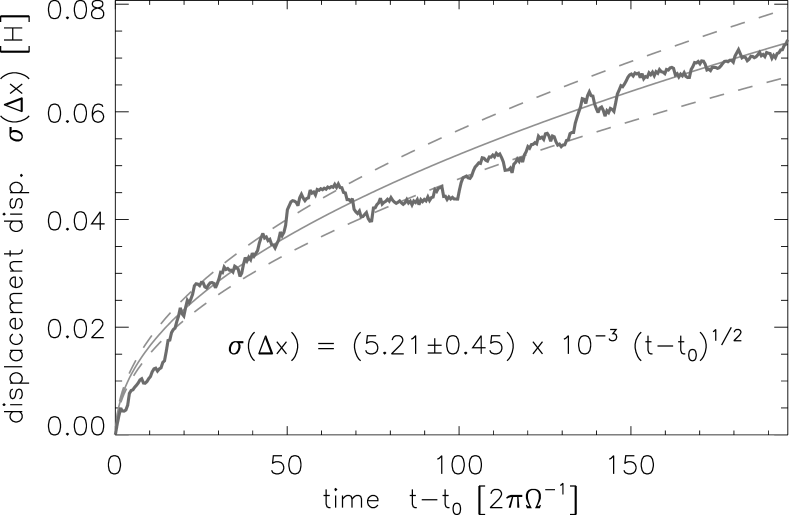
Figure 12: Dispersion of the radial displacement $\Delta x$ of a swarm of 25 test particles for run A1. The growing spread in the particles’ separation is well approximated by a random-walk as illustrated by the over-plotted curve.

6 Radial diffusion of planetesimals

It was shown in paper I that the radial drift of planetesimals of size $R_{\rm p}>10\,\rm km$ over typical disc life times due to gas drag is small. Instead, the diffusion of planetesimal semimajor axes is dominated by the stochastic gravitational torques exerted on the planetesimals by the turbulent disc. This implies that material of common origin and composition (e.g. planetesimals which form at a particular radial location in the disc), in time will spread out over a certain region in semimajor axis. The degree of spreading is determined by the disc life time and the strength of the stochastic torques.

In paper I, we examined the degree of spreading induced by the stochastic torques in a fully turbulent disc model similar in mass to the minimum mass solar nebula model, and showed that over a putative disc life time of $5\,\rm Myr$, planetesimals embedded in the current asteroid-belt region would spread inward and outward over a distance of $\sim 2.5\,\rm au$. Such a conclusion sits uncomfortably with the relatively low volatile content of the inner solar system planets (O’Brien et al., 2006), which would presumably be higher if substantial volatile-rich material from beyond the snow-line had migrated inward during the planet-forming epoch. Additionally, although the picture of how different taxonomic classes of asteroids are distributed as a function of heliocentric distance has become more complex in recent years (Mothé-Diniz et al., 2003), the earlier work of Gradie & Tedesco (1982) shows a clear trend of increasing volatile content as a function of heliocentric distance. In this latter study, the distribution of taxonomic types is consistent with a picture of in situ formation, followed by radial diffusion over a distance of $\simeq 0.5\,\rm au$. In the following discussion we judge that our models have had a measure of success if they do not violate the constraints implied by this picture.

In Fig. 12, we plot the evolution of the r.m.s. of the radial displacement of a swarm of test particles, and we find the resulting curve to be consistent with a random-walk. As mentioned above, we neglect dynamical interactions amongst the particles. This implies that self-stirring due to close encounters is not accounted for, and the given values have to be regarded as lower limits.

In Sect. 4, we have demonstrated that the gravitational torques acting on particles can be represented by a normal distribution, and their temporal correlations possess a finite coherence time. These two properties allow us to estimate particle diffusion based on a Fokker-Planck equation. As discussed in detail in section §3.7 of paper I (see also Johnson et al., 2006), the natural variable to describe this process is the specific angular momentum $j$. The time scale for diffusion of particle angular momenta due to stochastic torques is

$$t_{j}=\frac{(\Delta j)^{2}}{D_{j}}$$ (16)

where $D_{j}$ is the diffusion coefficient and $\Delta j$ is the change in $j$. The diffusion coefficient $D_{j}$ may be approximated by $D_{j}=\sigma_{\Gamma}^{2}\tau_{\rm c}$, where $\sigma_{\Gamma}$ is the r.m.s. of the fluctuating specific torques, and $\tau_{\rm c}$ is the correlation time associated with the fluctuating torques.

The change in specific angular momentum obtained after an evolution time of $t$ is given by

$$\Delta j=\sqrt{D_{j}\,t}.$$ (17)

Noting that small changes in specific angular momentum are related to small changes in the semi-major axis, $a$, by the expression

$$\frac{\Delta j}{j}=\frac{\Delta a}{2a}$$ (18)

the change in semimajor axis over an evolution time $t$ is:

$$\Delta a=\frac{2a\sqrt{D_{j}t}}{j}.$$ (19)

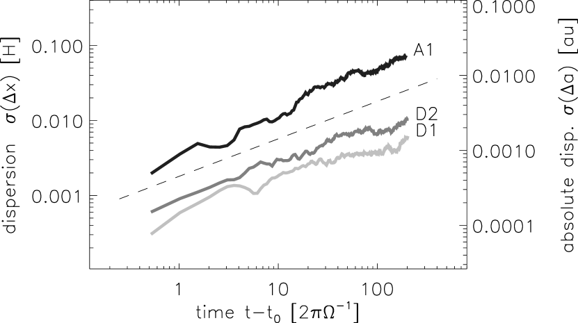
Figure 13: Model comparison for the random-walk behaviour shown in Fig. 12 above, but plotted logarithmically. The second axis gives the absolute dispersion $\Delta a$ at $r=5\,\rm au$. Evolution scaling with the square-root of time is indicated by the dashed line.

We can now examine the degree of agreement between the level of particle diffusion observed directly in the simulations, and presented in Fig. 13, and predictions based on (19). The radial location of the shearing box in our simulations is assumed to be $5\,\rm au$, and simulation run times are $t\simeq 200$ local orbits. The value of $D_{j}$ for each model may be computed using the expression $D_{j}=\sigma_{\Gamma}^{2}\tau_{\rm c}$, and values for $\sigma_{\Gamma}$, expressed in c.g.s. units, may be read off Fig. 8 for each model. The corresponding estimates of $\tau_{\rm c}$ are listed in Tab. 2 (along with the r.m.s. specific torques, $\sigma_{\Gamma}$).

We note that the time evolution of the r.m.s. radial displacement obtained in each model, $\sigma_{\Delta x}$, has been fitted using the expression

$$\sigma_{\Delta x}/H=C_{\sigma}(\Delta x)\sqrt{t}$$ (20)

where $H$ is the local disc thickness, the time $t$ is measured in units of local orbits, and the coefficients $C_{\sigma}(\Delta x)$ are tabulated in Tab. 2. After 200 orbits, the radial diffusion given by (20) corresponds to a change of semimajor axis $\Delta a=0.0184\,\rm au$ for model A1, which can be verified by inspection of Figure 13. The predicted change from (19) is $\Delta a=0.0122\,\rm au$, approximately 30% smaller than the observed value.

For model D1, we observe a change $\Delta a=0.00167\,\rm au$, and predict a change from (19) of $\Delta a=0.00161\,\rm au$, giving excellent agreement. For model D2, the observed change in semimajor axis is $\Delta a=0.00256\,\rm au$, which is approximately 25% smaller than the predicted value of $\Delta a=0.00336\,\rm au$. Taking these results overall, and noting that the use of only 25 particles in the simulations implies minimal sampling errors at the 20% level, we consider the agreement between the observed and predicted levels of diffusion to be very satisfactory.

Examining the longer term evolution, we use (20) to calculate the level of diffusion expected over an assumed disc life time of $5\,\rm Myr$. For the fully active model, A1, we obtain $\Delta a=2.9\,\rm au$, which is in good agreement with the result obtained in paper I. For model D1, we obtain $\Delta a=0.26\,\rm au$, and for model D2 we obtain $\Delta a=0.40\,\rm au$. It is clear from these values that in a vertically stratified disc sustaining MHD turbulence without a dead zone, radial diffusion is predicted to be too large to be consistent with solar system constraints. For a disc with a significant dead zone whose height extends either side of the midplane by a distance $\sim 2H$, however, we see that the degree of radial mixing is strongly diminished, and the results are consistent with the distribution of asteroidal taxonomic types (Gradie & Tedesco, 1982).

7 Discussion

We now attempt to summarise our results and present a coherent picture of how the dynamics and growth of planetesimals are affected by turbulent stirring in discs with and without dead zones. We frame our discussion in the context of the three planetesimal formation models discussed in the introduction: incremental growth through particle sticking over time scales exceeding $10^{5}\,\rm yr$ (Weidenschilling, 2000; Brauer et al., 2008); concentration of chondrules in turbulent eddies, followed by gravitational contraction on the chondrule settling time – typically $\sim 10^{2}$ - $10^{3}$ orbits (Cuzzi et al., 2008); gravitational collapse of dense clumps of metre-sized bodies formed in turbulent discs through a combination of trapping in local pressure maxima and the streaming instability (Johansen et al., 2007). Although there are significant problems with the incremental growth picture, in this paper we are interested in exploring the effects of turbulence on macroscopic bodies of sizes $R_{\rm p}\geq 100\,\rm m$, and so it is useful for our discussion to assume an optimistic outcome for this model. Toward the end of this section we also discuss some of the shortcomings of our model, and issues that are raised by these for the interpretation of our results.

7.1 Turbulent discs without dead zones

The results presented in Section 5 suggest that planetesimal formation and growth via a process involving mutual collisions between smaller bodies is not possible in fully turbulent discs. The rapid excitation of large random velocities which exceed the disruption/erosion threshold for planetesimals with $R_{\rm p}\leq 100\,\rm km$ will simply lead to the destruction of bodies which form in this manner. Although the turbulence simulated in this paper is quite vigorous, because of the imposed vertical magnetic field, the scaling developed in paper I for the strength of stochastic forcing as a function of the effective viscous stress suggest that even an order of magnitude decrease in the effective viscous $\alpha$ value will not decrease the random velocities sufficiently to prevent catastrophic disruption from occurring.

The formation of large ($R_{\rm p}\simeq 100\,\rm km$) planetesimals through chondrules concentrating in turbulent eddies may be possible in fully turbulent discs driven by the MRI. The obvious requirement for there to be a turbulent cascade resulting in Kolmogorov-scale eddies in which chondrules can concentrate would appear to be satisfied in such a disc. During the initial formation and settling stage of these objects, they are likely to be of low density and hence strongly coupled to the gas via gas drag. Relative velocities on local scales relevant for collisions are likely to be small. As they contract to form “sandpile” planetesimals, however, they will decouple from the gas and evolve dynamically like planetesimals with internal densities of $\rho_{\rm p}\simeq 2\,\rm g\,\rm cm^{-3}$. If formation/contraction times for these bodies are $\simeq 10^{4}\,\rm yr$ at $5\,\rm au$, then turbulent stirring will cause their velocity dispersion to grow to the surface escape velocity of $\simeq 100\,\rm m\,s^{-1}$ within $3.5\times 10^{4}\,\rm yr$, preventing runaway growth from ensuing. Further collisional growth between sandpile planetesimals will therefore occur slowly. Continued driving of the velocity dispersion by turbulence eventually allows $v_{\rm disp}$ to exceed the disruption value for $100\,\rm km$ rubble piles within approximately $1.2\,\rm Myr$. Clearly collisional growth must allow significantly larger bodies to form within this time to prevent the eventual collisional destruction of the majority of sandpile planetesimals. Even if larger bodies do form that are safe against collisional disruption, questions remain about the possibility of forming large planetary cores that can accrete gas within a few Myr in the absence of runaway growth. A model in which a relatively small number of large planetesimals avoid collisional destruction and grow by accreting the surrounding collisional debris may, however, provide a viable route to the growth of massive planetary cores.

Rapid formation of large planetesimals through the clumping of metre-size boulders, followed by their gravitational collapse, has been demonstrated in fully turbulent discs driven by the MRI (Johansen et al., 2007; Johansen et al., 2011). Although the size distribution of planetesimals arising from this process is not known accurately because of numerical limitations, the simulations produce objects with sizes similar to Ceres ($R_{\rm p}\simeq 500\,\rm km$). Such objects have surface escape velocities of $500\,\rm m\,s^{-1}$, and the time over which turbulent stirring generates a velocity dispersion of this magnitude is $\sim 8\times 10^{5}\,\rm yr$. It is unclear whether a population of planetesimals with an approximately unimodal size distribution centred on $R_{\rm p}=500\,\rm km$ can undergo runaway growth, because of self-stirring and weak gas drag damping of eccentricities. But if it is feasible then turbulent stirring in a fully active disc such as computed in model A1 will probably not provide significant hindrance because of the long time scales required for the velocity dispersion to grow above $v_{\rm disp}\simeq 500\,\rm m\,s^{-1}$.

7.2 Turbulent discs with dead zones

Our results for model D1 show that in a model with a relatively deep dead zone, the equilibrium velocity dispersion is determined by collisional rather than gas drag damping for bodies with $R_{\rm p}\leq 10\,\rm km$, for reasons discussed in section 5.3. The equilibrium velocity dispersion lies between the disruption/erosion thresholds for weak and strong aggregates, suggesting that incremental collisional growth of planetesimals is possible, but depends on the material strength of the bodies. For $100\,\rm m$ bodies, the time required to excite the velocity dispersion to the equilibrium value of $4.5\,\rm m\,s^{-1}$ is $\simeq 2.2\times 10^{4}\,\rm yr$, comfortably shorter than the formation time of km-sized planetesimals at $5\,\rm au$. Similarly, the time required to excite $1\,\rm km$ bodies to their equilibrium random velocities is $\simeq 2.2\times 10^{5}\,\rm yr$, comparable to our assumed formation time for these bodies through incremental growth. At each stage during the incremental growth of planetesimals within the dead zone, the planetesimals will have velocity dispersions close to the equilibrium values, which then control in-part the formation and growth rates. But provided the material strength of the planetesimals is sufficient (larger than that for weak aggregates), planetesimal growth should be possible in a dead zone through collisional agglomeration, so long as the bouncing and metre-size barriers can be overcome (Brauer et al., 2008; Zsom et al., 2010).

Runaway growth of km-sized planetesimals requires the velocity dispersion to be significantly lower than the escape velocity from the accreting bodies, and for $10\,\rm km$ planetesimals $v_{\rm esc}=10\,\rm m\,s^{-1}$. Results from model D1 indicate that a velocity dispersion of this magnitude will be excited within $\simeq 10^{5}\,\rm yr$, effectively quenching the runaway growth. Continued collisional growth can still proceed, since the velocity dispersion remains below the disruption/erosion threshold (at least for strong aggregates and rubble piles), and the equilibrium velocity dispersion for $10\,\rm km$ objects $v_{\rm disp}=51\,\rm m\,s^{-1}$ is not reached until after $2.2\,\rm Myr$. If growth ensues quickly enough, the eventual formation of bodies with $R_{\rm p}\simeq 100\,\rm km$ will allow runway growth of these planetesimals to occur. Model D1 shows that the time required to raise the velocity dispersion up to the escape velocity $v_{\rm esc}=100\,\rm m\,s^{-1}$ for these bodies is $10\,\rm Myr$. In this general picture, the influence of stochastic gravitational forces acting on planetesimals in a dead zone can cause the postponement of runaway growth for $10\,\rm km$ planetesimals, but once $100\,\rm km$ sized bodies form, rapid runaway growth produce numerous $\sim 1000\,\rm km$ sized oligarchs which will then undergo oligarchic growth to form planetary embryos and cores. This general picture of delayed runaway growth is similar in concept to that suggested by Kortenkamp et al. (2001) for planet formation in binary systems.

The formation of sandpile planetesimals via the concentration of chondrules within turbulent eddies should be possible in a dead zone, provided that the Reynolds stress generated there is indicative of a turbulent flow with an energy cascade resulting in Kolmogorov-eddies in which millimetre particles can become trapped. At the present time it is not clear that this is an accurate description of the dead zone flow, as the Reynolds stress appears to be largely due to spiral density waves that are stochastically excited in the disc active regions, and undergo non linear damping as their wavelengths shorten during radial propagation through the disc (Heinemann & Papaloizou, 2009b). A detailed analysis of high resolution simulations is required to examine the nature of the flow in the dead zone. Assuming that $100\,\rm km$ sandpile planetesimals can form, the slow growth of the velocity dispersion means that turbulent stirring cannot provide an impediment to subsequent runaway growth.

Similar comments apply to the rapid formation of planetesimals in dead zones via the mechanism described in Johansen et al. (2007). Formation in this case is driven to a large degree by trapping of metre-size bodies in pressure maxima (localised regions of anticyclonic vorticity) generated by turbulence (Johansen et al., 2011), and these are not as prominent in the midplane of a disc with a dead zone. This suggests that the streaming instability models in laminar discs presented in Johansen et al. (2009) may provide a more promising avenue for rapid planetesimal formation in dead zones. Once large planetesimals form, the possible onset of runaway growth will not be inhibited by the weak stochastic excitation of the velocity dispersion in a dead zone.

7.3 Caveats

We now consider the possible effects of assumptions we have made in our models that may affect their outcomes and the conclusions we have drawn from them.

7.3.1 Disc mass

The disc model we adopt in this study is lower in mass by a factor of $\sim 3$ than disc models that have been used as the basis for successful models of giant planet formation (Pollack et al., 1996). But it should be noted that these models often neglected the effects of planetary migration which can enable planetary embryos to grow beyond their isolation masses, thus assisting in the formation of giant planets within expected disc life times (Alibert et al., 2005). If relative density perturbations in the dead zone remain the same when the disc mass is increased, then a higher disc mass will lead to a corresponding increase in turbulent stirring, making planetesimal destruction/erosion more likely. But, in a disc where the ionisation sources are external (stellar X-rays, galactic cosmic rays), the column density and mass of the active zone are almost independent of the total disc mass/surface density, and depend primarily on the penetration depth of the ionising sources. Consequently, we may expect the relative density fluctuations near the midplane in the dead zone to be weaker in a heavier disc than in a lighter disc, potentially providing a less destructive source of gravitational stirring. At present it is unclear how turbulent stirring in a dead zone scales with the disc mass, and studying this issue is difficult from the computational point of view. The shearing box models we present here are extended in the $x$ and $y$ directions compared to those used in most studies, and include $\pm 5.5$ scale heights above and below the midplane. Increasing the disc mass moves the boundary between the dead and active zones further from the midplane, such that the vertical computational domain must be extended significantly to accommodate the active zone, increasing the computational expense. It is our intention to address this issue in a future study.

7.3.2 Initial magnetic fields

We have assumed a particular configuration for the initial magnetic fields in our simulations that includes a small but non-negligible net-flux vertical component. It is well known that the existence and strength of net-flux magnetic fields changes the saturation level of developed MHD turbulence in simulations of the MRI (Hawley et al., 1995). A future study of planetesimal dynamics embedded in turbulent discs with dead zones should examine the role played by the field topology and strength.

7.3.3 Planetesimal size distribution

In our estimates of collisional damping we assume that all planetesimals are the same size, and that all solids are incorporated into planetesimals. The latter assumption is broadly consistent with our disc model, in which we assume that 90% of the dust has been depleted due to the growth of grains into larger bodies. But the assumption of a single planetesimal size is not realistic. A more accurate calculation of the role of collisional damping would require a self-consistent model of accretion and fragmentation such that the size distribution is modelled self-consistently. Unfortunately such a model goes beyond the scope of this paper.

7.3.4 Planetesimal scale height

When estimating the scale height of the planetesimal disc during the calculation of collisional damping rates, we assumed that $H_{\rm p}=v_{\rm disp}/\Omega_{\rm k}$ (i.e. the velocity dispersion is isotropic). In a turbulent disc, however, where a significant component of the stochastic gravitational field is generated by spiral density waves that have little vertical structure, we should expect that the eccentricity growth exceeds that of the inclination. Our simulation results, however, show that for models D1 and D2 the inclination growth actually exceeds that of the eccentricity. This surprising result arises because the disc midplane (centre of mass in the $z$-direction), oscillates vertically with an amplitude that reaches $\sim 0.02H$, causing an oscillation of similar magnitude in the planetesimals. Future simulations of planetesimals within dead zones will be computed using global models to examine how robust this phenomenon is, although we note that a similar vertical oscillation has been reported in the shearing box simulations presented by Oishi et al. (2007).

7.4 Equation of state

Wave propagation in discs is strongly influenced by the equation of state (Lin et al., 1990; Korycansky & Pringle, 1995). This may affect the ability of waves that are excited in the active regions to propagate into the dead zone, and thus affect the turbulent stirring there. The simulations presented in this paper all adopted an isothermal equation of state, whereas protoplanetary discs are expected to be optically thick at $5\,\rm au$.

For parameters typical of T Tauri stars, the primary heating mechanism near the midplane is the absorption of the radiation emitted by the disc atmosphere, which in turn heats mainly by absorbing light from the central star (Chiang & Goldreich, 1997). The accretion heating also occurs in the atmosphere, leading to a thoroughly isothermal interior when a dead zone is present (Hirose & Turner, 2011). The role of the equation of state in determining the level of turbulent stirring at the midplane will be explored in a future publication.

8 Conclusions

In this paper we have presented the results of simulations of planetesimals embedded in local models of protoplanetary discs. The main aim of this work is to understand the dynamics of planetesimals in turbulent discs, and to examine how dead zones of varying vertical thicknesses change the stochastic forcing of the radial velocity dispersion, and the diffusion of planetesimal semimajor axes. We consider the influence of gas drag and collisional damping in counteracting the growth of random velocities due to turbulent stirring, and estimate the equilibrium velocity dispersions which result. The main conclusions of this study are as follows.

The presence and depth of a dead zone have negligible effect on the measured coherence time of the particle stirring, but only affect its amplitude as measured through the width of the torque distribution.

In fully turbulent discs without dead zones, we find that the velocity dispersion of embedded planetesimals grows rapidly, and quickly exceeds the threshold for disruption for planetesimals in the size range $100\,\rm m\leq R_{\rm p}\leq 10\,\rm km$. We conclude that planetesimal formation via collisional accretion of smaller bodies cannot occur in globally turbulent discs. The direct formation of large $100\,\rm km$-sized planetesimals via turbulent concentration and gravitational instability (Johansen et al., 2007; Cuzzi et al., 2008) may occur, but the excitation of their random velocities may prevent runaway growth, making it difficult to form large planetary embryos and cores within reasonable disc life times.

Radial diffusion of planetesimals occurs over distances of $\sim 2.5\,\rm au$ in fully turbulent discs over typical disc life times of $5\,\rm Myr$. This is inconsistent with the observed correlation between asteroid taxonomic types and heliocentric distance in the asteroid belt, which indicate radial mixing over distances $\leq 0.5\,\rm au$ during the formation of the solar system. It thus seems implausible that the solar nebula sustained levels of turbulence observed in numerical simulations of fully turbulent discs.

The stochastic forcing of planetesimal random motions is much weaker in discs with dead zones. In a dead zone with vertical extent $\pm 2H$ above and below the midplane, the stochastic excitation of planetesimal eccentricities is reduced by a factor $\sim 17$ relative to a fully active disc. The damping of planetesimal random motions in this model is dominated by collisional damping, and the equilibrium velocity dispersions lie between the disruption thresholds for weak and strong aggregates. It thus appears that the collisional growth and formation of km-sized planetesimals may be possible in a dead zone. But, we note that the tidal break-up of comet Shoemaker-Levy 9 (Asphaug & Benz, 1996), and analysis of the collision ejecta from comet Tempel 1 during the Deep Impact mission (Richardson et al., 2007), suggest that cometary bodies possess modest material strength. It therefore remains uncertain what range of collision velocities can be tolerated during the incremental growth of km-sized planetesimals as envisaged in the models of Weidenschilling (2000) and Brauer et al. (2008).

Although km-sized planetesimals may be able form within a dead zone, subject to overcoming the metre-sized and bouncing barriers, stochastic forcing by the turbulent disc excites random velocities above the escape velocity for $R_{\rm p}=10\,\rm km$ bodies within $10^{5}\,\rm yr$, quenching runaway growth. Slower growth of planetesimals through collisions remains possible, and runaway growth can ensue once bodies with $R_{\rm p}\simeq 100\,\rm km$ form, due to the slow growth of random velocities within a dead zone. If $R_{\rm p}\simeq 1000\,\rm km$ ‘oligarchs’ form, oligarchic growth can proceed with very modest influence from the weak stochastic forcing in the dead zone. A corollary of this is that $100\,\rm km$-sized planetesimals that form through the concentration of particles and subsequent gravitational instability in a dead zone will not be prevented from undergoing runaway growth by turbulent stirring.

In summary, we come to the following specific conclusions regarding the outcome of our present study:

• Comparing the results obtained for dead zones with different vertical heights ($\sim 1.5H$ and $2H$), we find that the larger dead zone model clearly favours the collisional formation of planetesimals because of weaker stochastic forcing of random motions.

• The radial diffusion of planetesimals is much reduced in discs with dead zones relative to fully active discs. Diffusion over a distance equal to $0.26\,\rm au$ is predicted by our deeper dead zone model, consistent with solar system constraints.

• The low diffusion levels for planetesimal semimajor axes in dead zones clearly means that stochastic torques in such an environment cannot prevent the large scale inward drift of low mass planets via type I migration.

• We suggest that dead zones provide safe havens for km-sized planetesimals against destructive collisions, and are probably a required ingredient for the formation of planetary systems.

This paper is part of series in which we are examining the dynamics of planetesimals and planets in increasingly realistic disc models, and shows that different qualitative outcomes for planet formation can be expected in discs with dead zones versus those without. In future publications we will examine a number of issues, including how changing the disc surface density and the mass ratio between the active and dead zones modifies the turbulent stirring, and how turbulence varies as a function of heliocentric distance in global MHD simulations of protoplanetary discs.

References

- Alibert et al. (2005) Alibert Y., Mordasini C., Benz W., Winisdoerffer C., 2005, A&A, 434, 343
- Armitage (1998) Armitage P. J., 1998, ApJ, 501, L189+
- Asphaug & Benz (1996) Asphaug E., Benz W., 1996, Icarus, 121, 225
- Balbus & Hawley (1991) Balbus S. A., Hawley J. F., 1991, ApJ, 376, 214
- Balsara & Meyer (2010) Balsara D. S., Meyer C., 2010, (astro-ph:1003.0018)
- Baruteau & Lin (2010) Baruteau C., Lin D. N. C., 2010, ApJ, 709, 759
- Benz & Asphaug (1999) Benz W., Asphaug E., 1999, Icarus, 142, 5
- Blaes & Balbus (1994) Blaes O. M., Balbus S. A., 1994, ApJ, 421, 163
- Brandenburg (2008) Brandenburg A., 2008, AN, 329, 725
- Brandenburg et al. (2009) Brandenburg A., Candelaresi S., Chatterjee P., 2009, MNRAS, 398, 1414
- Brauer et al. (2008) Brauer F., Dullemond C. P., Henning T., 2008, A&A, 480, 859
- Bridges et al. (1984) Bridges F. G., Hatzes A., Lin D. N. C., 1984, Nature, 309, 333
- Chiang & Goldreich (1997) Chiang E. I., Goldreich P., 1997, ApJ, 490, 368
- Courvoisier et al. (2010) Courvoisier A., Hughes D. W., Proctor M. R. E., 2010, AN, 331, 667
- Cuzzi et al. (2008) Cuzzi J. N., Hogan R. C., Shariff K., 2008, ApJ, 687, 1432
- Davis et al. (2010) Davis S. W., Stone J. M., Pessah M. E., 2010, ApJ, 713, 52
- Flaig et al. (2010) Flaig M., Kley W., Kissmann R., 2010, MNRAS, 409, 1297
- Fleming & Stone (2003) Fleming T., Stone J. M., 2003, ApJ, 585, 908
- Fleming et al. (2000) Fleming T. P., Stone J. M., Hawley J. F., 2000, ApJ, 530, 464
- Flock et al. (2010) Flock M., Dzyurkevich N., Klahr H., Mignone A., 2010, A&A, 516, A26+
- Fromang et al. (2002) Fromang S., Terquem C., Balbus S. A., 2002, MNRAS, 329, 18
- Gammie (1996) Gammie C. F., 1996, ApJ, 457, 355
- Gardiner & Stone (2005) Gardiner T. A., Stone J. M., 2005, JCoPh, 205, 509
- Garmire et al. (2000) Garmire G., Feigelson E. D., Broos P., Hillenbrand L. A., Pravdo S. H., Townsley L., Tsuboi Y., 2000, AJ, 120, 1426
- Glassgold et al. (1997) Glassgold A. E., Najita J., Igea J., 1997, ApJ, 480, 344
- Goldreich & Ward (1973) Goldreich P., Ward W. R., 1973, ApJ, 183, 1051
- Gradie & Tedesco (1982) Gradie J., Tedesco E., 1982, Science, 216, 1405
- Gressel (2010) Gressel O., 2010, MNRAS, 405, 41
- Gressel & Ziegler (2007) Gressel O., Ziegler U., 2007, CoPhC, 176, 652
- Haisch et al. (2001) Haisch Jr. K. E., Lada E. A., Lada C. J., 2001, ApJ, 553, L153
- Hanasz et al. (2009) Hanasz M., Otmianowska-Mazur K., Kowal G., Lesch H., 2009, A&A, 498, 335
- Hawley (2001) Hawley J. F., 2001, ApJ, 554, 534
- Hawley et al. (1995) Hawley J. F., Gammie C. F., Balbus S. A., 1995, ApJ, 440, 742
- Hayashi (1981) Hayashi C., 1981, Progress of Th. Phys. Suppl., 70, 35
- Heinemann & Papaloizou (2009a) Heinemann T., Papaloizou J. C. B., 2009a, MNRAS, 397, 52
- Heinemann & Papaloizou (2009b) Heinemann T., Papaloizou J. C. B., 2009b, MNRAS, 397, 64
- Hirose & Turner (2011) Hirose S., Turner N. J., 2011, ApJ, 732, L30
- Ida et al. (2008) Ida S., Guillot T., Morbidelli A., 2008, ApJ, 686, 1292
- Ida & Makino (1993) Ida S., Makino J., 1993, Icarus, 106, 210
- Igea & Glassgold (1999) Igea J., Glassgold A. E., 1999, ApJ, 518, 848
- Ilgner & Nelson (2006a) Ilgner M., Nelson R. P., 2006a, A&A, 445, 205
- Ilgner & Nelson (2006b) Ilgner M., Nelson R. P., 2006b, A&A, 445, 223
- Ilgner & Nelson (2008) Ilgner M., Nelson R. P., 2008, A&A, 483, 815
- Johansen et al. (2011) Johansen A., Klahr H., Henning T., 2011, A&A, 529, A62+
- Johansen & Levin (2008) Johansen A., Levin Y., 2008, A&A, 490, 501
- Johansen et al. (2007) Johansen A., Oishi J. S., Low M., Klahr H., Henning T., Youdin A., 2007, Nature, 448, 1022
- Johansen et al. (2009) Johansen A., Youdin A., Mac Low M., 2009, ApJ, 704, L75
- Johnson et al. (2006) Johnson E. T., Goodman J., Menou K., 2006, ApJ, 647, 1413
- Kenyon & Bromley (2009) Kenyon S. J., Bromley B. C., 2009, ApJ, 690, L140
- Kokubo & Ida (1998) Kokubo E., Ida S., 1998, Icarus, 131, 171
- Kortenkamp et al. (2001) Kortenkamp S. J., Wetherill G. W., Inaba S., 2001, Science, 293, 1127
- Korycansky & Pringle (1995) Korycansky D. G., Pringle J. E., 1995, MNRAS, 272, 618
- Latter et al. (2010) Latter H. N., Fromang S., Gressel O., 2010, MNRAS, 406, 848
- Latter et al. (2009) Latter H. N., Lesaffre P., Balbus S. A., 2009, MNRAS, 394, 715
- Lin et al. (1990) Lin D. N. C., Papaloizou J. C. B., Savonije G. J., 1990, ApJ, 364, 326
- Miller & Stone (2000) Miller K. A., Stone J. M., 2000, ApJ, 534, 398
- Miyoshi & Kusano (2005) Miyoshi T., Kusano K., 2005, JCoPh, 208, 315
- Mothé-Diniz et al. (2003) Mothé-Diniz T., Carvano J. M. Á., Lazzaro D., 2003, Icarus, 162, 10
- Nelson (2005) Nelson R. P., 2005, A&A, 443, 1067
- Nelson & Gressel (2010) Nelson R. P., Gressel O., 2010, MNRAS, 409, 639
- Nelson & Papaloizou (2004) Nelson R. P., Papaloizou J. C. B., 2004, MNRAS, 350, 849
- O’Brien et al. (2006) O’Brien D. P., Morbidelli A., Levison H. F., 2006, Icarus, 184, 39
- Oishi et al. (2007) Oishi J. S., Mac Low M., Menou K., 2007, ApJ, 670, 805
- Papaloizou & Nelson (2003) Papaloizou J. C. B., Nelson R. P., 2003, MNRAS, 339, 983
- Pessah & Goodman (2009) Pessah M. E., Goodman J., 2009, ApJ, 698, L72
- Pollack et al. (1996) Pollack J. B., Hubickyj O., Bodenheimer P., Lissauer J. J., Podolak M., Greenzweig Y., 1996, Icarus, 124, 62
- Regev & Umurhan (2008) Regev O., Umurhan O. M., 2008, A&A, 481, 21
- Rheinhardt & Brandenburg (2010) Rheinhardt M., Brandenburg A., 2010, A&A, 520, A28+
- Richardson et al. (2007) Richardson J. E., Melosh H. J., Lisse C. M., Carcich B., 2007, Icarus, 190, 357
- Rüdiger & Pipin (2000) Rüdiger G., Pipin V. V., 2000, A&A, 362, 756
- Sano et al. (2000) Sano T., Miyama S. M., Umebayashi T., Nakano T., 2000, ApJ, 543, 486
- Shi et al. (2010) Shi J., Krolik J. H., Hirose S., 2010, ApJ, 708, 1716
- Sicilia-Aguilar et al. (2004) Sicilia-Aguilar A., Hartmann L. W., Briceño C., Muzerolle J., Calvet N., 2004, AJ, 128, 805
- Stewart & Leinhardt (2009) Stewart S. T., Leinhardt Z. M., 2009, ApJ, 691, L133
- Stone & Gardiner (2010) Stone J. M., Gardiner T. A., 2010, ApJS, 189, 142
- Stone et al. (1996) Stone J. M., Hawley J. F., Gammie C. F., Balbus S. A., 1996, ApJ, 463, 656
- Turner & Drake (2009) Turner N. J., Drake J. F., 2009, ApJ, 703, 2152
- Turner & Sano (2008) Turner N. J., Sano T., 2008, ApJ, 679, L131
- Turner et al. (2007) Turner N. J., Sano T., Dziourkevitch N., 2007, ApJ, 659, 729
- Umebayashi (1983) Umebayashi T., 1983, Progress of Theoretical Physics, 69, 480
- Umebayashi & Nakano (1981) Umebayashi T., Nakano T., 1981, PASJ, 33, 617
- Umebayashi & Nakano (2009) Umebayashi T., Nakano T., 2009, ApJ, 690, 69
- Wardle (1999) Wardle M., 1999, MNRAS, 307, 849
- Weidenschilling (1977) Weidenschilling S. J., 1977, MNRAS, 180, 57
- Weidenschilling (2000) Weidenschilling S. J., 2000, Space Sci. Rev., 92, 295
- Weidenschilling & Cuzzi (1993) Weidenschilling S. J., Cuzzi J. N., 1993, in E. H. Levy & J. I. Lunine eds., Protostars and Planets III, Univ. Arizona Press, Tucson, p. 1031
- Wetherill & Stewart (1993) Wetherill G. W., Stewart G. R., 1993, Icarus, 106, 190
- Yang et al. (2009) Yang C., Mac Low M., Menou K., 2009, ApJ, 707, 1233
- Youdin & Goodman (2005) Youdin A. N., Goodman J., 2005, ApJ, 620, 459
- Ziegler (2004) Ziegler U., 2004, JCoPh, 196, 393
- Ziegler (2008) Ziegler U., 2008, CoPhC, 179, 227
- Zsom et al. (2010) Zsom A., Ormel C. W., Güttler C., Blum J., Dullemond C. P., 2010, A&A, 513, A57+