Time-dependent quantum transport and power-law decay of the transient current in a nano-relay and nano-oscillator

Abstract

Time-dependent nonequilibrium Green’s functions are used to study electron transport properties in a device consisting of two linear chain leads and a time-dependent interleads coupling that is switched on non-adiabatically. We derive a numerically exact expression for the particle current and examine its characteristics as it evolves in time from the transient regime to the long-time steady-state regime. We find that just after switch-on the current initially overshoots the expected long-time steady-state value, oscillates and decays as a power law, and eventually settles to a steady-state value consistent with the value calculated using the Landauer formula. The power-law parameters depend on the values of the applied bias voltage, the strength of the couplings, and the speed of the switch-on. In particular, the oscillating transient current decays away longer for lower bias voltages. Furthermore, the power-law decay nature of the current suggests an equivalent series resistor-inductor-capacitor circuit wherein all of the components have time-dependent properties. Such dynamical resistive, inductive, and capacitive influences are generic in nano-circuites where dynamical switches are incorporated. We also examine the characteristics of the dynamical current in a nano-oscillator modeled by introducing a sinusoidally modulated interleads coupling between the two leads. We find that the current does not strictly follow the sinusoidal form of the coupling. In particular, the maximum current does not occur during times when the leads are exactly aligned. Instead, the times when the maximum current occurs depend on the values of the bias potential, nearest-neighbor coupling, and the interleads coupling.

I INTRODUCTION

The further miniaturization of electronic devices will eventually lead to molecular electronics wherein particles pass through molecular-scale devices whose constituent molecules may have been manipulated and synthetically assembled or created.heath03 Molecular transistors, in particular, are of significant practical interests and whose successful implementations are currently actively being pursued. Several theoretical models of the transistor have been proposedpalacios02 ; ghosh04 and experimental successes have also been reported.kubatkin03 A related molecular-scale device, the molecular switch, has also garnered significant interests because of the switch’s important role in circuit design and architecture. A theoretical model of the switch makes use of a mechanism that involves the reversible displacement of an atom in a molecular wire through the application of a gate voltage.wada93 In addition, experimental realizations of the atomic switch include mechanisms involving the reversible transfer of an atom between two leads,eigler91 the dynamical onset of single-atom contact between leadsterabe05 and the manipulation of atomic bonds using a dynamic force microscope.sweetman11 Having a dynamical switch in a nano-circuit, however, necessitates the appearance of time-dependent behavior, particularly during the transient regime just after switch-on. The circuit transitions from being disconnected into connected in a short time and the current does not instantly switches into the steady-state value upon connection. It is therefore informative to know the characteristics of the current just after switch-on and during the transient regime, and determine how this current approaches the steady-state value. In this work, we introduce a model device representing a system wherein the current can be dynamically toggled on and off. There are several theoretical approaches in treating time-dependent quantum transport. Among these include time-dependent density functional theory,runge84 propagating the Kadanoff-Baym equations,prociuk08 Floquet theory,moskalets02 path-integral techniques,altland10 and the density matrix renormalization group method.branschadel10 ; karrasch10 ; pletyukhov10 In this work we choose to use time-dependent nonequilibrium Green’s functions (TD-NEGF) because, as is shown in this paper, dynamically toggling the coupling between the leads is straightforward using the technique, even without the assumption of weak coupling, and the resulting expression for the time-dependent current is numerically exact.

Figure 1: (Color online) (a) An illustration of the nano-relay and nano-oscillator. The left lead is firmly on a stationary substrate and the right lead is on a rotatable disk. The left and right leads align when the disk is rotated clockwise to the dash line. (b) The device can be represented by two semi-infinite leads connected by a time-varying coupling $v^{\rm LR}(t)$ switched on at $t=0$. In both leads, the on-site energy is $\epsilon$ and the nearest-neighbor hopping parameter is $v$. (c) An equivalent resistor-inductor-capacitor circuit with dynamical properties.

The device we examine consists of a semi-infinite linear chain of atoms, i.e., the left lead, which is stationary and another semi-infinite linear chain of atoms, i.e., the right lead, that is on a rotatable disk. An illustration of the device is shown in Fig. 1(a). When the disk is rotated clockwise to the dashed line, the left and right leads align and conduction occurs. We model how the two leads couple in two ways: as an abrupt Heaviside step function and as a hyperbolic tangent that gradually progresses in time. For such cases, the off state has no current flowing across the leads. In addition, we can also model an oscillator by swinging the disk back and forth across the dashed line. The rotatable disk can also be replaced by a gate voltage, located on top of the right lead, that could rotate the right lead to its desired position. This latter configuration has previously been examined and, in particular, the steady-state transport properties of its on and off states have been studied ghosh04 . In this paper, however, we study the full time-dependent transport properties of the device. Numerically exact expressions for the current and the needed nonequilibrium Green’s functions are derived. We then show that just after switch-on and during the transient regime the current initially overshoots the expected value of the steady-state current and then oscillates around the steady-state value while decaying as a power law. Such a power-law decaying transient current suggests the appearance of dynamical resistance, inductance, and capacitance in the system during the transient regime. Power-law decaying currents have also recently been predicted to appear in a system containing a quantum dot channelkarrasch10 and in the anisotropic Kondo model.pletyukhov10

II MODEL AND METHOD

We implement time-dependent nonequilibrium Green’s functions techniques to investigate the dynamical transport properties of particles traversing through a device with time-varying components. To determine the dynamical transport properties, a TD-NEGF approach can be used that utilizes either two-timejauho94 ; haug07 Green’s functions, or double-energyanantram95 Green’s functions, or Green’s functions that depend on one time and one energy variables.arrachea05a ; arrachea05b In a transistor with source-channel-drain and top gate configuration, for example, the device can be modeled by a Hamiltonian constructed using density functional theoryzhu05 ; ke10 or tight-binding theorymoldoveanu07 and the dynamical transport properties of small channels are calculated using TD-NEGF. For devices with larger channels, a self-consistent calculation based on the Poisson equation and TD-NEGF can be done to determine the consistent dynamical potential and charge density in the channel.kienle09 In this work, in contrast, we study a device consisting only of two leads, i.e., there is no channel between the leads. The time-dependence comes from non-adiabatically toggling on the coupling between the leads. We use TD-NEGF to derive a numerically exact expression for the dynamical current and investigate how the devices we call a nano-relay and a nano-oscillator respond to time-varying influences. This approach has recently also been used in the study of dynamical heat transport in a thermal switchcuansing10 .

We model the system by the total Hamiltonian $H=H^{\rm L}+H^{\rm R}+H^{\rm LR}$, where $H^{\rm L}$ is for the left lead on the stationary substrate, $H^{\rm R}$ is for the right lead on the rotatable disk, and $H^{\rm LR}$ includes the dynamic interleads coupling. In the leads, particles follow the tight-binding Hamiltonian

$$H^{\alpha}=\sum_{k}\epsilon_{k}^{\alpha}~{}c_{k}^{\alpha\dagger}c_{k}^{\alpha}+\sum_{kj}v_{kj}^{\alpha}~{}c_{k}^{\alpha\dagger}c_{j}^{\alpha},~{}~{}\alpha={\rm L,R},$$ (1)

where $c_{k}^{\alpha\dagger}$ and $c_{k}^{\alpha}$ are particle creation and annihilation operators at the $k$th site in the $\alpha$ lead. $\epsilon_{k}$ is the on-site energy at site $k$ and $v_{kj}$ is the hopping parameter between nearest-neighbor sites $k$ and $j$ (see Fig. 1(b)). The sums are over all sites in the $\alpha$ lead. $H^{\rm LR}$ includes the time-dependent component of the total Hamiltonian and is of the form

$$H^{\rm LR}=\sum_{kj}\left(v_{kj}^{\rm LR}~{}c_{k}^{{\rm L}\dagger}c_{j}^{\rm R}+v_{jk}^{\rm RL}~{}c_{j}^{{\rm R}\dagger}c_{k}^{\rm L}\right),$$ (2)

where $v_{jk}^{\rm LR}(t)=v_{kj}^{\rm RL}(t)$ is the time-dependent coupling between the left and right leads and is switched-on at $t=0$. Only the right-most site of the left lead, i.e., the site labeled $0$ in Fig. 1(b), can couple to the left-most site of the right lead, i.e., the site labeled $1$ in the figure.

The current can be determined by noting how the number operator, $N^{\alpha}=\sum_{k}c_{k}^{\alpha\dagger}c_{k}^{\alpha}$, changes with time, i.e., $I^{\rm R}(t)=-q\left<dN^{\rm R}/dt\right>$, where $q$ is the electron charge. Defining the two-time lesser Green’s function as

$$G_{jk}^{{\rm RL},<}(t_{1},t_{2})=\frac{i}{\hbar}\left<c_{k}^{{\rm L}\dagger}(t_{2})~{}c_{j}^{\rm R}(t_{1})\right>,$$ (3)

we can write the electron current flowing out of the right lead as

$$I^{\rm R}(t)=-\frac{iq}{\hbar}\sum_{kj}\left(v_{kj}^{\rm LR}\left<c_{k}^{{\rm L}\dagger}c_{j}^{\rm R}\right>-v_{jk}^{\rm RL}\left<c_{j}^{{\rm R}\dagger}c_{k}^{\rm L}\right>\right)=-2q{\rm Re}\left(\sum_{kj}v_{kj}^{\rm LR}~{}G_{jk}^{{\rm RL},<}(t,t)\right).$$ (4)

Similar steps can be done to determine the current flowing out of the left lead. We find $I^{\rm L}(t)=-I^{\rm R}(t)$ and therefore, current is always conserved at each instant of time $t$.

We define the contour-ordered Green’s function

$$G_{jk}^{\rm RL}(\tau_{1},\tau_{2})=-\frac{i}{\hbar}\left<{\rm T}_{c}~{}c_{j}^{\rm R}(\tau_{1})c_{k}^{{\rm L}\dagger}(\tau_{2})\right>,$$ (5)

where T_c is the contour-ordering operator and $\tau_{1}$ and $\tau_{2}$ are variables along the contour.haug07 Since we want to calculate the current for both the steady-state and non-steady-state regimes, we employ a contour that begins at $t=0$ when the interleads coupling has just been switched on, then proceeds to time $t$ where we want to determine the current, and then goes back to time $t=0$. In the interaction picture the contour-ordered Green’s function can be expanded in powers of $i/{\hbar}$. Applying Wick’s theorem to the resulting expansion and then using Langreth’s theorem and analytic continuation,haug07 we get a numerically exact expression that includes all terms in the expansion for the lesser Green’s function:

$$\begin{split}G_{jk}^{{\rm RL},<}(t_{1},t_{2})={}&G_{jk,1}^{{\rm RL},<}(t_{1},t_{2})+~{}\sum_{mn}\int_{0}^{t}dt^{\prime}~{}G_{jm}^{{\rm RL},r}(t_{1},t^{\prime})v_{mn}^{\rm LR}(t^{\prime})G_{nk,1}^{{\rm RL},<}(t^{\prime},t_{2})\\ &+~{}\sum_{mn}\int_{0}^{t}dt^{\prime}~{}G_{jm,1}^{{\rm RL},<}(t_{1},t^{\prime})v_{mn}^{\rm LR}(t^{\prime})G_{nk}^{{\rm RL},a}(t^{\prime},t_{2})\\ &+~{}\sum_{mnpq}\int_{0}^{t}dt^{\prime}\int_{0}^{t}dt^{\prime\prime}~{}G_{jm}^{{\rm RL},r}(t_{1},t^{\prime})v_{mn}^{\rm LR}(t^{\prime})G_{np,1}^{{\rm RL},<}(t^{\prime},t^{\prime\prime})v_{pq}^{\rm LR}(t^{\prime\prime})G_{qk}^{{\rm RL},a}(t^{\prime\prime},t_{2}),\end{split}$$ (6)

where the advanced and retarded Green’s functions are

$$G_{jk}^{{\rm RL},\zeta}(t_{1},t_{2})=G_{jk,1}^{{\rm RL},\zeta}(t_{1},t_{2})+~{}\sum_{mn}\int_{0}^{t}dt^{\prime}~{}G_{jm,1}^{{\rm RL},\zeta}(t_{1},t^{\prime})v_{mn}^{\rm LR}(t^{\prime})G_{nk}^{{\rm RL},\zeta}(t^{\prime},t_{2}),~{}~{}\zeta=r,a.$$ (7)

The first-order retarded and advanced Green’s functions are

$$G_{jk,1}^{{\rm RL},\zeta}(t_{1},t_{2})=\int_{0}^{t}dt^{\prime}~{}g_{jj}^{{\rm R},\zeta}(t_{1}-t^{\prime})v_{jk}^{\rm RL}(t^{\prime})g_{kk}^{{\rm L},\zeta}(t^{\prime}-t_{2}),$$ (8)

and the first-order lesser Green’s function is

$$G_{jk,1}^{{\rm RL},<}(t_{1},t_{2})=\int_{0}^{t}dt^{\prime}\left\{g_{jj}^{{\rm R},r}(t_{1}-t^{\prime})v_{jk}^{\rm RL}(t^{\prime})g_{kk}^{{\rm L},<}(t^{\prime}-t_{2})+g_{jj}^{{\rm R},<}(t_{1}-t^{\prime})v_{jk}^{\rm RL}(t^{\prime})g_{kk}^{{\rm L},a}(t^{\prime}-t_{2})\right\},$$ (9)

where the $g^{r}(t)$, $g^{a}(t)$, and $g^{<}(t)$ are the retarded, advanced, and lesser free-leads Green’s functions, respectively. Time-translation invariance is satisfied by the free leads and therefore, their corresponding Green’s functions can be calculated in the energy domain using the techniques of steady-state NEGF.datta05 The integrals in Eqs. (8) and (9) are then determined using the extended Simpson’s rule algorithm for numerical integration.press07 Furthermore, the expressions for the advanced and retarded Green’s functions in Eq. (7) are in the form of a Fredholm equation of the second kind and can be solved by discretizing the time integrals, based on the extended Simpson’s rule algorithm, and performing a matrix inversion using LU (lower-triangular and upper-triangular) decomposition.press07 The lesser Green’s function can then be calculated from the retarded and advanced Green’s function by applying the extended Simpson’s rule algorithm to numerically solve the integrals in Eq. (6).

III RESULTS AND DISCUSSION

Firstly, we examine the impact of the switch-on speed to current characteristics. The functional form of the interleads coupling, $v^{\rm LR}(t)$, describes how the device is switched on. We examine two types of switch-ons: an abrupt Heaviside step function switch-on and a gradually progressing hyperbolic tangent switch-on of the form $v^{\rm LR}(t)=v^{\rm LR}\tanh(\omega_{d}t)$, where $\omega_{d}$ is the driving frequency. The step function switch-on is actually the limit when $\omega_{d}\rightarrow\infty$ of the hyperbolic tangent switch-on. Furthermore, we set the on-site energy $\epsilon=0$. The left and right leads have temperature $T^{\rm L}=T^{\rm R}=300~{}{\rm K}$ and chemical potential $\mu_{\rm L}=\epsilon_{F}$ and $\mu_{\rm R}=\epsilon_{F}-qV_{b}$, where we set the Fermi energy $\epsilon_{F}=0$. The bias potential $V_{b}$ is applied to the right lead and the bias potential energy is written as $U_{b}=qV_{b}$.

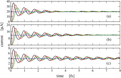
Figure 2: (Color online) The current as a function of time when the interleads coupling $v^{\rm LR}(t)$ is switched on as a step function at $t=0$ (black lines), gradually as a hyperbolic tangent with driving frequency $\omega_{d}=0.5~{}{\rm[1/t]}$ (red lines), and $\omega_{d}=0.25~{}{\rm[1/t]}$ (green lines), where ${\rm[1/t]}=10^{16}~{}{\rm rad/s}$. The bias potentials are ${\rm(a)}~{}U_{b}=0.5~{}{\rm eV}$, ${\rm(b)}~{}U_{b}=0.3~{}{\rm eV}$, and ${\rm(c)}~{}U_{b}=0.1~{}{\rm eV}$. The (blue) dashed lines are the values of the steady-state current. The hopping parameter in the leads is $v=-2.7~{}{\rm eV}$.

Figure 2 shows the current flowing out of the left lead for the step function and hyperbolic tangent switch-on with driving frequencies $\omega_{d}=0.25~{}{\rm[1/t]}$ and $0.5~{}{\rm[1/t]}$, where ${\rm[1/t]}=10^{16}~{}{\rm rad/s}$. The steady-state values of the current calculated separately using the Landauer formula for a linear chain with unit transmissiondatta97 are also shown in Fig. 2 as dashed lines. During the times just after the switch-on, the current rapidly increases and overshoots the expected long-time steady-state value. It then oscillates and decays in time, eventually settling to the steady-state value. It can be seen that as the driving frequency is decreased the amplitude of the oscillations also decreases. In addition, the peaks are displaced to later times because of the more gradual progress of the interleads coupling $v^{\rm LR}(t)$. In Fig. 2 we also see the dependence of the decay time of the transient current to the applied bias potential and the speed of the switch-on. The higher bias results in a faster decay time for the oscillating transient current.

The transient current oscillates and decays in time until it settles to a steady-state value.dc During the transient regime the strength of the interleads coupling dynamically changes resulting in particles temporarily accumulating at the left and right sides of that coupling. Although we do not explicitly consider Coulomb interactions between charges, the temporary accumulation of charges at the sides of the interleads coupling, together with the distance between the accumulated charges and the applied bias voltage across the interleads coupling, can be regarded to generate a temporary dynamical capacitance. Similarly, a dynamical inductance may arise because the transient current is varying in time. By considering possible equivalent circuit combinations and performing least-squares fitting to the envelope of the decaying transient current we find that the decay closely follows a power law, indicating an equivalent series resistor-inductor-capacitor (RLC) circuit whose components have time-dependent properties. In a previous study using semiclassical Boltzmann transport theory on quantum wires, it is found that the wire can be modeled by an equivalent series RLC circuit.salahuddin05 A series RLC circuit consisting of components with constant resistance, inductance, and capacitance results in a transient current whose envelope decays as an exponential function. However, when the resistance, inductance, and capacitance vary in time, the resulting transient current can oscillate and could decay as a power law. Making therefore such an analogy to the quantum device we are examining (see Fig. 1(c)), applying Kirchhoff’s law to a series RLC circuit with time-varying components leads to the equation

$$\frac{d^{2}I}{dt^{2}}+\left(\frac{R}{L}+\frac{1}{L}\frac{dL}{dt}\right)\frac{dI}{dt}+\left(\frac{1}{L}\frac{dR}{dt}+\frac{1}{LC}\right)I=\frac{Q}{LC^{2}}\frac{dC}{dt},$$ (10)

where $I$ is the time-dependent current through the circuit, $R\equiv R(t)$ is the resistance, $L\equiv L(t)$ is the inductance, $C\equiv C(t)$ is the capacitance, and $Q=\int_{0}^{t}I~{}dt$ is the time-dependent charge accumulating at the capacitor. Furthermore, the power law fits imply that the current is of the form

$$I(t)=I_{0}~{}t^{-\alpha}\sin(\omega t+\phi)+I_{0},$$ (11)

where $\alpha$ is the power-law exponent determined from the fits, $\omega$ is the time-independent frequency of oscillation of the transient current, $\phi$ is the phase determined from initial conditions, and $I_{0}$ is the time-independent steady-state current. Taking the time derivative of Eq. (11) twice, we find

$$\frac{d^{2}I}{dt^{2}}+\frac{2\alpha}{t}\frac{dI}{dt}+\omega_{t}^{2}I=\omega_{t}^{2}I_{0},$$ (12)

where $\omega_{t}^{2}=\omega^{2}+\frac{\alpha(\alpha-1)}{t^{2}}$. Comparing Eqs. (10) and (12) we get the coupled equations

$$\begin{split}\frac{R}{L}+\frac{1}{L}\frac{dL}{dt}={}&\frac{2\alpha}{t},\\ \frac{1}{L}\frac{dR}{dt}+\frac{1}{LC}={}&\omega_{t}^{2},\\ \frac{Q}{LC^{2}}\frac{dC}{dt}={}&\omega_{t}^{2}I_{0},\end{split}$$ (13)

which can be solved to determine how $R(t)$, $L(t)$, and $C(t)$ vary in time for specific values of $\alpha$ and $\omega$.

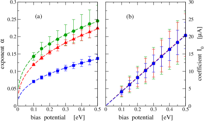
Figure 3: (Color online) (a) The power-law exponent $\alpha$ and (b) coefficient $I_{0}$ as functions of the bias potential. The (green) dots are for the Heaviside step function interleads coupling. The (red) triangles are for the hyperbolic tangent interleads coupling with $\omega_{d}=0.5~{}{\rm[1/t]}$. The (blue) squares are for $\omega_{d}=0.25~{}{\rm[1/t]}$. The dashed lines are power-law fits to the corresponding data points. The amplitude of the couplings are $v=v^{\rm LR}=-2.7~{}{\rm eV}$. Error bars arise from the difference between values from the top and bottom envelopes.

The power-law exponent $\alpha$ determines how fast the transient current decays until it reaches the steady-state value. In Fig. 3(a), it can be observed that by increasing the bias potential the value of $\alpha$ also increases, thereby speeding up the decay of the transient current. $\alpha$ and the power-law coefficient $I_{0}$ actually also follow power-law fits when the bias potential is varied, as can be seen in Fig. 3. It suggests $\alpha=\alpha_{0}~{}U_{b}^{\beta}$ and $I_{0}=I_{00}~{}U_{b}^{\gamma}$, where $\alpha_{0}$ and $I_{00}$ are independent of $U_{b}$. The power-law exponents $\beta$ and $\gamma$ determine how fast $\alpha$ and $I_{0}$, respectively, change when the bias potential is varied. In Table 1 we show how the values of the power-law fitting parameters change when $U_{b}$ is varied.

Table 1: Values from the power-law fits to $\alpha$ and $I_{0}$ when the interleads coupling is in the form of a hyperbolic tangent and a step function. The couplings are $v=-2.7~{}{\rm eV}$ and $v^{\rm LR}=-2.7~{}{\rm eV}$. The dimension of $\alpha_{0}$ is $(1/{\rm eV})^{\beta}$ and $I_{00}$ is $\mu{\rm A}/({\rm eV})^{\gamma}$.

$\omega_{d}$ [1/t]	$\alpha_{0}$	$\beta$	$I_{00}$	$\gamma$
0.25	0.181	0.416	40.753	0.999
0.5	0.292	0.392	40.684	0.989
(step)	0.307	0.332	40.214	0.983

From Table 1, we see that the values of $I_{00}$ and $\gamma$ are independent of the speed of the switch-on. In addition, the exponent $\gamma$ is about one. These imply that $I_{0}$ increases linearly with the bias potential and is consistent with the identification that $I_{0}$ is the steady-state current. For the exponent $\alpha$, we find that as the speed of the switch-on is increased the coefficient $\alpha_{0}$ also increases but the exponent $\beta$ decreases. The increasing $\alpha_{0}$ suggests that for a given bias potential, the faster switch-on results in a faster decay of the transient current. Since the slightly decreasing $\beta$ is still positive, increasing the bias potential still speeds up the decay of the transient current. As a result, when the device is operated under low bias its current suffers oscillations and overshootings longer than when it is operated under higher bias. Furthermore, it can be observed that the power-law parameters $\alpha_{0}$ and $\beta$ control the speed of decay of the transient current. The values of these two parameters vary depending on the speed of the switch-on. If we want the system to have a fast decaying transient current, then our results indicate that we need a switch-on that is as fast as possible.

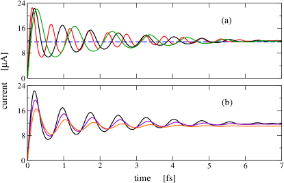
Figure 4: (Color online) The current as a function of time for a step function switch-on. (a) The couplings have values $v=v^{\rm LR}=-4.0~{}{\rm eV}$ (red line), $v=v^{\rm LR}=-2.7~{}{\rm eV}$ (black line), and $v=v^{\rm LR}=-2.0~{}{\rm eV}$ (green line). The (blue) dashed line is the value of the steady-state current. (b) The hopping parameter is fixed at $v=-2.7~{}{\rm eV}$ and the interleads coupling is varied with values $v^{\rm LR}=-2.7~{}{\rm eV}$ (black line), $v^{\rm LR}=-2.4~{}{\rm eV}$ (violet line), and $v^{\rm LR}=-2.1~{}{\rm eV}$ (orange line). The bias potential for both plots is $U_{b}=0.3~{}{\rm eV}$.

Next, we investigate the effects of varying the values of the hopping parameter $v$ and the interleads coupling $v^{\rm LR}$. The values of these tight-binding parameters depend on the material used and varying them effectively means that we change the material we use for the device. The parameters can be varied separately or they can be varied while maintaining $v=v^{\rm LR}$. Firstly, we consider the latter case. In order to determine only the effects of varying the couplings, and not the effects of the speed of the switch-on, we employ the step function switch-on. The current as a function of time is shown in Fig. 4(a). Since $v=v^{\rm LR}$, the long-time steady-state values of the current can be calculated from the Landauer formula with a transmission coefficient $T=1$ (no scattering involved). This steady-state value is shown in Fig. 4(a) as a dashed line. We examine coupling values $v=v^{\rm LR}=-2.0~{}{\rm eV},-2.7~{}{\rm eV}$, and $-4.0~{}{\rm eV}$. The bias potential is fixed at $U_{b}=0.3~{}{\rm eV}$. We find that as the couplings become more negative the frequency of oscillation of the transient current increases. The decrease in the value of the couplings imply that the energy needed for the particle to hop from one site to a neighboring site is decreased. This frees up the particle, thereby allowing higher oscillation frequencies in the transient current. For long times after the transient oscillations have decayed away, the steady-state value of the current is independent of the specific value of the couplings.

Furthermore, we examine the effects of varying $v$ and $v^{\rm LR}$ separately. When $v^{\rm LR}$ is different from $v$, the interleads distance is different from the nearest-neighbor distance between sites in the leads. This results in a potential barrier that is different at the interleads coupling and thus, a particle moving from the left lead scatters at the interleads coupling. Figure 4(b) shows the current as a function of time when the nearest-neighbor hopping parameter is set at $v=-2.7~{}{\rm eV}$ and we vary $v^{\rm LR}$ to values $-2.7~{}{\rm eV}$, $-2.4~{}{\rm eV}$, and $-2.1~{}{\rm eV}$. We do not consider $\left|v^{\rm LR}\right|>\left|v\right|$ values because that would imply a shorter interleads distance than the natural nearest-neighbor distance, represented by $v$, in the leads. In contrast, decreasing $\left|v^{\rm LR}\right|$ increases the potential barrier at the interleads coupling, and thus implying a longer interleads distance, and results in the reduction in the amplitude of the oscillating transient current. From Fig. 4(b), we also see that the peaks are slightly shifted to later times. In addition, the long-time steady-state current slightly decreases when $\left|v^{\rm LR}\right|$ is decreased. If we want to calculate the steady-state current using the Landauer formula, we would find that the transmission coefficient is reduced when $v^{\rm LR}$ is different from $v$ because of the scattering occuring at the interleads coupling.

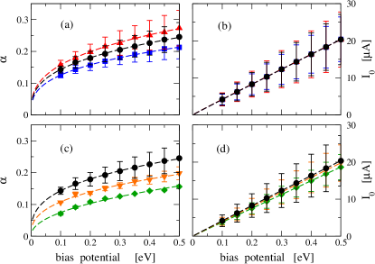
Figure 5: (Color online) The exponent $\alpha$ and coefficient $I_{0}$ when $v$ and $v^{\rm LR}$ are varied. In (a) and (b), $v=v^{\rm LR}=-2.0~{}{\rm eV}$ for the (red triangles), $v=v^{\rm LR}=-2.7~{}{\rm eV}$ for the (black dots), and $v=v^{\rm LR}=-4.0~{}{\rm eV}$ for (blue squares). In (c) and (d), we set $v=-2.7~{}{\rm eV}$ and vary $v^{\rm LR}$ to values $-2.1~{}{\rm eV}$ (green diamonds), $-2.4~{}{\rm eV}$ (orange inverted triangles), and $-2.7~{}{\rm eV}$ (black dots). The dashed lines are the power-law fits to the corresponding data points.

The oscillating and decaying transient current when $v$ and $v^{\rm LR}$ are varied also follow a power law. In Figs. 5(a) and 5(b) the values of $v$ and $v^{\rm LR}$ are varied together while in Figs. 5(c) and 5(d) the values are varied separately. Figure 5(b) shows that the values of $I_{0}$ is the same for the cases examined. Compared to Fig. 5(d), we see that the values of $I_{0}$ are slightly different. Identifying $I_{0}$ as the steady-state current, we thus confirm that it is the same whenever $v=v^{\rm LR}$. On the other hand, the scattering that happens at the interleads coupling when $v^{\rm LR}$ is different from $v$ affects the value of the steady-state current. Moreover, the plots of the exponent $\alpha$ and coefficient $I_{0}$ as functions of the bias potential can also be fitted to power laws. As shown in Table 2, when $v=v^{\rm LR}$, decreasing the value of the couplings decreases both the coefficient $\alpha_{0}$ and the exponent $\beta$, while $I_{00}$ and $\gamma$ remain the same. The transient current therefore decays slower. This is because decreasing the couplings decreases the energy required for the particle to move around. This increase in the particle’s freedom to move increases the frequency of oscillation and slightly lengthens the decay of the transient current. However, fixing the value of $v$ and increasing $v^{\rm LR}$ decreases $\alpha_{0}$ and $I_{00}$, but increases $\beta$. Therefore, for a given bias potential, increasing $v^{\rm LR}$ lengthens the decay but suppresses the amplitude of oscillation of the transient current. The parameters $\alpha_{0}$, $\beta$, $I_{00}$, and $\gamma$ depend on the type of material used. The value of the interleads coupling $v^{\rm LR}$, in addition, depends on the distance between the leads. The farther apart are the two leads, the higher is the value of $v^{\rm LR}$ because of the higher interleads potential barrier. Our results show that stronger interleads scattering lengthens the decay of the transient current. However, the scattering also suppresses the amplitude of the transient current and decreases the eventual value of the long-time steady-state current.

Table 2: (Color online) Values from the power-law fits to the exponent $\alpha$ as a function of the bias potential $U_{b}$ when the switch-on of the interleads coupling is in the form of a Heaviside step function. The shaded entries indicate cases when $v\neq v^{\rm LR}$. The dimension of $\alpha_{0}$ is $(1/{\rm eV})^{\beta}$ and $I_{00}$ is $\mu{\rm A}/({\rm eV})^{\gamma}$.

$v$ [eV]	$v^{\rm LR}$ [eV]	$\alpha_{0}$	$\beta$	$I_{00}$	$\gamma$
-2.0	-2.0	0.344	0.340	40.125	0.980
-2.7	-2.7	0.307	0.332	40.214	0.983
-4.0	-4.0	0.268	0.330	40.305	0.985
-2.7	-2.1	0.219	0.466	37.152	0.993
-2.7	-2.4	0.252	0.367	39.344	0.992

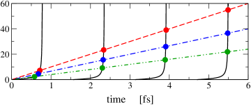
Figure 6: (Color online) The location of the peaks in the transient current. The (black) lines represent $\tan(\omega~{}t+\phi)$, where $\omega=2~{}{\rm[1/t]}$ and $\phi=\pi$. The (red) dashed line represents $\omega~{}t/\alpha$, where $\alpha=0.2$. The (blue) dashed-dot line is when $\alpha=0.3$ and the (green) dashed-double dot line is when $\alpha=0.5$. The times when the straight and tangent lines intersect correspond to the times when the peaks in the transient current occur.

The times when the peaks in the current occur can be known from the extremum of the power-law form of the current in Eq. (11). Taking the time derivative of Eq. (11) and then equating the result to $0$, we find the extremum of the current to occur at times $t_{p}$ whenever the following is satisfied:

$$\frac{\omega~{}t_{p}}{\alpha}=\tan\left(\omega~{}t_{p}+\phi\right).$$ (14)

The left-hand side is an equation for a straight line with a slope that depends on $\alpha$. Since $\alpha$ varies depending on the values of the bias potential, the couplings, and the speed of the switch-on, changing these parameters would change the slope. As a consequence, the location in time of the current peaks would also change. This can be seen by noting how the peaks in the transient current move in Fig. 2 as $\alpha$ is varied. $t_{p}$ can be determined by the intersection points of the straight and tangent lines, corresponding to the left-hand side and right-hand side, respectively, of Eq. (14) and as shown in Fig. 6. The times when the current peaks occur are located whenever the two curves intersect. Since the slope of the straight line depends on $\alpha$, we see that the faster decaying transient current, i.e., higher values of $\alpha$, correspond to earlier peak times.

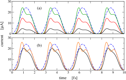
Figure 7: (Color online) The current as a function of time for the nano-oscillator with driving frequency $\omega_{d}=0.25~{}{\rm[1/t]}$. (a) The bias potentials are $U_{b}=0.1~{}{\rm eV}$ (black line), $U_{b}=0.3~{}{\rm eV}$ (red line), and $U_{b}=0.5~{}{\rm eV}$ (green line). The couplings are $v=v^{\rm LR}=-2.7~{}{\rm eV}$. (b) The bias potential is $U_{b}=0.5~{}{\rm eV}$ and the hopping parameter is $v=-2.7~{}{\rm eV}$. The interleads coupling has amplitudes $v^{\rm LR}=-2.1~{}{\rm eV}$ (black line) and $v^{\rm LR}=-3.0~{}{\rm eV}$ (orange line). The (blue) dashed lines show the harmonic variation of the interleads coupling. Their amplitudes are not drawn to scale.

Finally, we investigate the transport properties of the device having a regular time variation, such as a nano-oscillator. In a nano-oscillator, the rotating disk in Fig. 1(a) is rocked back and forth across the dashed line. This would result in a harmonic modulation of the interleads coupling and would dynamically modulate the current through the device. However, compared to an alternating current which changes sign, the modulated current flowing out of the nano-oscillator maintains the same sign. We model the harmonically modulated coupling in the form $v^{\rm LR}(t)=v^{\rm LR}/2\cdot\left(1-\cos\omega_{d}t\right)$, where $\omega_{d}$ is the driving frequency of modulation. Figure 7 shows the current characteristics as a function of time as the interleads coupling is swinged back and forth with driving frequency $\omega_{d}=0.25~{}{\rm[1/t]}$. In Fig. 7(a), the couplings are $v=v^{\rm LR}=-2.7~{}{\rm eV}$ and the bias potential is varied. In Fig. 7(b) the bias potential is set at $U_{b}=0.5~{}{\rm eV}$, the hopping parameter is fixed at $v=-2.7~{}{\rm eV}$, and the interleads coupling $v^{\rm LR}$ is varied. We find that the current through the oscillator comes in pulses. However, it does not exactly follow the harmonic form of the coupling. The interleads coupling is maximum at times when the left and right leads are exactly aligned. In contrast, we see that the peaks in the current do not coincide with the times when the interleads coupling is maximum. The shape of the curve for the current actually looks like the truncated version of the transient current we examined in Fig. 2. In particular, the initial overshoot of the transient current manifests as the first current peak in Fig. 7. This peak, however, does not occur when the interleads coupling is maximum. In addition, the times when the peak occurs depend on the values of the bias potential and the couplings. This dependence of the peak location to the above physical parameters follow similar dependence of the peak location in the nano-relay. In the design of nano-circuits containing an oscillator, therefore, it should be noted that the maximum current does not occur when the leads are exactly aligned and that the exact location of these peaks depend on the values of the applied bias potential, the nearest-neighbor coupling, and the interleads coupling.

IV SUMMARY AND CONCLUSION

In summary, we examine a device that could act as a nano-relay or a nano-oscillator. The device consists of two leads and a time-varying interleads coupling. We use NEGF to derive a nonperturbative expression for the time-dependent current flowing from one lead to the other. In the nano-relay configuration, we model the switch-on of the interleads coupling in the form of either a step function or a slowly progressing hyperbolic tangent. We find that the current oscillates and decays in time just after switch-on and during the transient regime. In both the step function and hyperbolic tangent switch-on, the decay of the transient current fits a power law. This leads to an equivalent RLC series circuit where all of the components have dynamical properties. We also find that the values of the couplings $v$ and $v^{\rm LR}$, the scattering at the interleads coupling, the speed of the switch-on, and the value of the bias potential affect the decay time of the transient current. In the long-time regime, the current approaches the steady-state value. In the nano-oscillator, we model the dynamical sytem by harmonically modulating the interleads coupling. We find that the current passes through the device in pulses, maintains the same sign, but does not exactly follow the functional form of the oscillating coupling. In particular, the peaks in the current do not occur at the times whenever the leads are exactly aligned.

The expressions for the current shown in Eq. (4) and the corresponding lesser Green’s function shown in Eq. (6) are general and should be applicable to transport in quasi-linear systems where a switch-on in time occurs. The current oscillates and decays as a power law after a switch-on. This power-law decay implies the presence of dynamical resistance, inductance, and capacitance components.

- (1) J.R. Heath and M.A. Ratner, Phys. Today 56, 43 (2003).
- (2) J.J. Palacios, A.J. Pérez-Jiménez, E. Louis, E. SanFabián, and J.A. Vergés, Phys. Rev. B 66, 035322 (2002); T. Rakshit, G.-C. Liang, A.W. Ghosh, and S. Datta, Nano Lett. 4, 1803 (2004).
- (3) A.W. Ghosh, T. Rakshit, and S. Datta, Nano Lett. 4, 565 (2004).
- (4) S. Kubatkin, A. Danilov, M. Hjort, J. Cornil, J.-L. Brédas, N. Stuhr-Hansen, P. Hedegård, and T. Bjørnholm, Nature 425, 698 (2003). S.J. Tans, A.R.M. Verschueren, and C. Dekker, ibid. 393, 49 (1998); H. Song, Y. Kim, Y.H. Jang, H. Jeong, M.A. Reed, and T. Lee, ibid. 462, 1039 (2009); N.J. Tao, Nature Nanotech. 1, 173 (2006).
- (5) Y. Wada, T. Uda, M. Lutwyche, S. Kondo, and S. Heike, J. Appl. Phys. 74, 7321 (1993).
- (6) D.M. Eigler, C.P. Lutz, and W.E. Rudge, Nature 352, 600 (1991).
- (7) K. Terabe, T. Hasegawa, T. Nakayama, and M. Aono, Nature 433, 47 (2005); C.A. Martin, R.H.M. Smit, H.S.J. van der Zant, and J.M. van Ruitenbeek, Nano Lett. 9, 2940 (2009).
- (8) A. Sweetman, S. Jarvis, R. Danza, J. Bamidele, S. Gangopadhyay, G.A. Shaw, L. Kantorovich, and P. Moriarty, Phys. Rev. Lett. 106, 136101 (2011).
- (9) E. Runge and E.K.U. Gross, Phys. Rev. Lett. 52, 997 (1984); G. Stefanucci, Phys. Rev. B 69, 195318 (2004); N. Bushong, N. Sai, and M. Di Ventra, Nano Lett. 5, 2569 (2005).
- (10) A. Prociuk and B.D. Dunietz, Phys. Rev. B 78, 165112 (2008); P. Myöhänen, A. Stan, G. Stefanucci, and R. van Leeuwen, Europhys. Lett. 84, 67001 (2008); ibid., Phys. Rev. B 80, 115107 (2009).
- (11) M. Moskalets and M. Büttiker, Phys. Rev. B 66, 205320 (2002); ibid. 69, 205316 (2004); ibid. 72, 035324 (2005); S. Kohler, J. Lehmann, and P. Hänggi, Phys. Rep. 406, 379 (2005); L. Arrachea and M. Moskalets, Phys. Rev. B 74, 245322 (2006).
- (12) A. Altland, A. De Martino, R. Egger, and B. Narozhny, Phys. Rev. B 82, 115323 (2010).
- (13) A. Branschädel, G. Schneider, and P. Schmittekert, Ann. Phys. (Berlin) 522, 657 (2010).
- (14) C. Karrasch, S. Andergassen, M. Plethukhov, D. Schuricht, L. Borda, V. Meden, and H. Schoeller, Eur. Phys. Lett. 90, 30003 (2010).
- (15) M. Pletyukhov, D. Schuricht, and H. Schoeller, Phys. Rev. Lett. 104, 106801 (2010).
- (16) A.-P. Jauho, N.S. Wingreen, and Y. Meir, Phys. Rev. B 50, 5528 (1994).
- (17) H. Haug and A.-P. Jauho, Quantum Kinetics in Transport and Optics of Semiconductors, 2nd ed. (Springer, Berlin, 2007).
- (18) M.P. Anantram and S. Datta, Phys. Rev. B 51, 7632 (1995); B. Wang, J. Wang, and H. Guo, Phys. Rev. Lett. 82, 398 (1999).
- (19) L. Arrachea, Phys. Rev. B 72, 125349 (2005); ibid. 75, 035319 (2007).
- (20) L. Arrachea, Phys. Rev. B 72, 121306(R) (2005).
- (21) Y. Zhu, J. Maciejko, T. Ji, H. Guo, and J. Wang, Phys. Rev. B 71, 075317 (2005); J. Maciejko, J. Wang, and H. Guo, ibid. 74, 085324 (2006); Z. Feng, J. Maciejko, J. Wang, and H. Guo, ibid. 77, 075302 (2008); B. Wang, Y. Xing, L. Zhang, and J. Wang, ibid. 81, 121103(R) (2010); Y. Xing, B. Wang, and J. Wang, ibid. 82, 205112 (2010).
- (22) S.-H. Ke, R. Liu, W. Yang, and H.U. Baranger, J. Chem. Phys. 132, 234105 (2010).
- (23) V. Moldoveanu, V. Gudmundsson, and A. Manolescu, Phys. Rev. B 76, 085330 (2007); V. Moldoveanu, V. Gudmundsson, and A. Manolescu, ibid. 76, 165308 (2007).
- (24) D. Kienle and F. Léonard, Phys. Rev. Lett. 103, 026601 (2009); D. Kienle, M. Vaidyanathan, and F. Léonard, Phys. Rev. B 81, 115455 (2010).
- (25) E.C. Cuansing and J.-S. Wang, Phys. Rev. B 81, 052302 (2010); E.C. Cuansing and J.-S. Wang, ibid. 83, 019902(E) (2011); E.C. Cuansing and J.-S. Wang, Phys. Rev. E 82, 021116 (2010).
- (26) S. Datta, Quantum Transport: Atom to Transistor, 2nd ed. (Cambridge University Press, Cambridge, U.K., 2005).
- (27) W.H. Press, S.A. Teukolsky, W.T. Vetterling, and B.P. Flannery, Numerical Recipes: The Art of Scientific Computing, 3rd ed. (Cambridge University Press, New York, 2007).
- (28) S. Datta, Electronic Transport in Mesoscopic Systems (Cambridge University Press, Cambridge, U.K., 1997).
- (29) It is relevant to notice in Fig. 2 that the current approaches a non-zero steady-state value during later times. This indicates the presence of a dc component in the current and is due to the applied static bias voltage between the left and right leads. The dc component vanishes when there is no applied bias voltage. If a dc component in the current is desired without the application of a bias voltage between the leads (and assuming that the leads have the same chemical potentials), then it is necessary to break time-reversal and spatial-inversion symmetry in the system.arrachea05b
- (30) S. Salahuddin, M. Lundstrom, and S. Datta, IEEE Trans. Electron Devices 52, 1734 (2005).