Report: IFIC/11-18, FTUV-11-0419


Three-particle correlations in QCD jets and beyond


Redamy Pérez-Ramos 111e-mail: redamy.perez@uv.es, Vincent Mathieu 222e-mail: vincent.mathieu@ific.uv.es and Miguel-Angel Sanchis-Lozano 333e-mail: miguel.angel.sanchis@ific.uv.es

Departament de Física Teòrica and IFIC, Universitat de València - CSIC

Dr. Moliner 50, E-46100 Burjassot, Spain


Abstract: In this paper, we present a more detailed version of our previous work for three-particle correlations in quark and gluon jets [1]. We give theoretical results for this observable in the double logarithmic approximation and the modified leading logarithmic approximation. In both resummation schemes, we use the formalism of the generating functional and solve the evolution equations analytically from the steepest descent evaluation of the one-particle distribution. In addition, in this paper we include predictions beyond the limiting spectrum approximation and study this observable near the hump of the single inclusive distribution. We thus provide a further test of the local parton hadron duality (LPHD) and make predictions for the LHC. The computation of higher rank correlators is presented in the double logarithmic approximation and shown to be rather cumbersome.

1 Introduction

The observation of quark and gluon jets has played a crucial role in establishing Quantum Chromodynamics (QCD) as the theory of strong interaction within the Standard Model of particle physics [2, 3]. Jets, narrowly collimated bundles of hadrons, reflect configurations of quarks and gluons at short distances [4, 5].

The evolution of gluon and quark initiated jets is dominated by soft gluon bremsstrahlung. Powerful schemes, like the Double Logarithmic Approximation (DLA) and the Modified Leading Logarithmic Approximation (MLLA), which allow for the perturbative resummation of soft-collinear and hard-collinear gluons before the hadronization occurs, have been developed over the past thirty years (for a review see [6]). In the frame of high energy jets, one of the strikest predictions of perturbative QCD (pQCD), which follows as a consequence of Angular Ordering (AO) within the MLLA and the Local Parton Hadron Duality (LPHD) hypothesis [7], is the existence of the hump-backed shape [8] of the inclusive energy distribution of hadrons, later confirmed by experiments at colliders like the LEP [9, 10] and the Tevatron [11]. Within the same formalism, the transverse momentum distribution, or ksubscript𝑘perpendicular-tok_{\perp}-spectra of hadrons produced in pp¯𝑝¯𝑝p\bar{p} collisions at center of mass energy s=1.96 TeV𝑠1.96 TeV\sqrt{s}=1.96\text{ TeV} at the Tevatron [12], was well described by MLLA [13] and next-to-MLLA (NMLLA) [14, 15] predictions inside the validity ranges provided by such schemes, both supported by the LPHD. Thus, the study and tests of enough inclusive observables like the inclusive energy distribution and the inclusive transverse momentum ksubscript𝑘perpendicular-tok_{\perp} spectra of hadrons have shown that the perturbative stage of the process, which evolves from the hard scale or leading parton virtuality QEsimilar-to𝑄𝐸Q\sim E to the hadronization scale Q0subscript𝑄0Q_{0}, is dominant. In particular, these issues suggest that the hadronization stage of the QCD cascade do not affect pQCD predictions and therefore, that the LPHD hypothesis is successful while treating one-particle inclusive observables.

The study of particle correlations in intrajet cascades, which are less inclusive observables, provide a refined test of the partonic dynamics and the LPHD. In [16], the two-particle correlations inside quark and gluon jets were first computed at DLA. In [18, 17], this observable was computed for the first time at MLLA for such particles, whose energy or x𝑥x (energy fraction of the jet carried away by one parton) stays close to the maximum of the one-particle distribution. In [19], the previous solutions were extended, at MLLA, to all possible values of x𝑥x by exactly solving the QCD evolution equations. This observable was measured by the OPAL collaboration in the e+esuperscript𝑒superscript𝑒e^{+}e^{-} annihilation at the Z0superscript𝑍0Z^{0} peak, that is for s=91.2 GeV𝑠91.2 GeV\sqrt{s}=91.2\text{ GeV} at LEP [20]. Though the agreement with predictions presented in [19] turned out to be rather good for the description of the data [20], a discrepancy still subsists pointing out a possible failure of the LPHD for less inclusive observables. However, these measurements were redone by the CDF collaboration in pp¯𝑝¯𝑝p\bar{p} collisions at the Tevatron for mixed samples of quark and gluon jets [11]. The agreement with predictions presented in [18, 17] turned out to be rather good, in particular for very soft particles (x0.1much-less-than𝑥0.1x\ll 0.1) having very close energy fractions (x1x2subscript𝑥1subscript𝑥2x_{1}\approx x_{2}). A discrepancy between the OPAL and CDF analysis showed up and still stays unclear. That is why, the measurement of two-particle correlations at the LHC becomes crucial.

By going one step beyond, in this paper we give predictions for three-particle correlations inside quark and gluon jets. This observable together with two-particle correlations can be measured in equal footing at the LHC. Such tests will provide further verifications of the LPHD for less inclusive observables and shed more light on the role of confinement in jet evolution. Further issues on the importance of correlations versus single-particle distributions studies have been presented in [21, 22].

The paper is organized as follows.

  • in section 2 we recall the formalism of jet generating functionals and their evolution equations;

  • the kinematics and the process for the inclusive production of three particles inside the jet are specified in subsection 2.1 and 2.1.1 respectively;

  • in subsection 2.2, we obtain the MLLA exact system of integro-differential evolution equations for the three-particle correlations and in subsection 2.3, the single logarithms (SLs) contributions are obtained from the exact evolution equations;

  • in subsection 2.4, we obtain the DLA solution of the evolution equations and study the shape and overall normalization of this observable;

  • in subsection 2.5 the evolution equations are solved iteratively and the solution are expressed in terms of the logarithmic derivatives of the one-particle distribution and the two-particle correlations;

  • in subsection 2.6, we finally give the analytical predictions which will be displayed in order to provide predictions for the Tevatron and the LHC;

  • in subsection 2.7, the hump approximation is applied to this observable;

  • in subsection 2.8, the region in x𝑥x where the emission of three correlated particles becomes dominant is discussed;

  • in subsection 2.9, we give the analytical solution of the DLA four-particle correlator and show that including higher order corrections for differential higher rank correlators would become a cumbersome task;

  • in subsection 3, the predictions are displayed and the phenomenology is applied to the Tevatron and the LHC;

  • a conclusion summarizes this work; the appendices are written as complements of the main core of the paper.

2 Formalism of the generating functional

A generating functional Z(E,Θ;{u})𝑍𝐸Θ𝑢Z(E,\Theta;\{u\}) can be constructed [23] that describes the azimuth averaged parton content of a jet of energy E𝐸E with a given opening half-angle ΘΘ\Theta; by virtue of the exact angular ordering (MLLA), it satisfies the following integro-differential evolution equation [6]

ddlnΘZA(p,Θ;{u})𝑑𝑑Θsubscript𝑍𝐴𝑝Θ𝑢\displaystyle\frac{d}{d\ln\Theta}Z_{A}\left(p,\Theta;\{u\}\right)\!\! =\displaystyle\!\!=\!\! 12B,C01𝑑zΦAB[C](z)αs(k2)π12subscript𝐵𝐶superscriptsubscript01differential-d𝑧superscriptsubscriptΦ𝐴𝐵delimited-[]𝐶𝑧subscript𝛼𝑠subscriptsuperscript𝑘2perpendicular-to𝜋\displaystyle\!\!\frac{1}{2}\sum_{B,C}\int_{0}^{1}dz\>\Phi_{A}^{B[C]}(z)\ \frac{\alpha_{s}\left(k^{2}_{\perp}\right)}{\pi} (2)
(ZB(zp,Θ;{u})ZC((1z)p,Θ;{u})ZA(p,Θ;{u}));subscript𝑍𝐵𝑧𝑝Θ𝑢subscript𝑍𝐶1𝑧𝑝Θ𝑢subscript𝑍𝐴𝑝Θ𝑢\displaystyle\Big{(}Z_{B}\big{(}zp,\Theta;\{u\}\big{)}\ Z_{C}\big{(}(1-z)p,\Theta;\{u\}\big{)}-Z_{A}\big{(}p,\Theta;\{u\}\big{)}\Big{)};

in (2), z𝑧z and (1z)1𝑧(1-z) are the energy-momentum fractions carried away by the two offspring in the ABC𝐴𝐵𝐶A\to BC parton decay described by the standard one loop splitting functions [24]

Φqq[g](z)=CF1+z21z,Φqg[q](z)=CF1+(1z)2z,formulae-sequencesuperscriptsubscriptΦ𝑞𝑞delimited-[]𝑔𝑧subscript𝐶𝐹1superscript𝑧21𝑧superscriptsubscriptΦ𝑞𝑔delimited-[]𝑞𝑧subscript𝐶𝐹1superscript1𝑧2𝑧\displaystyle\Phi_{q}^{q[g]}(z)=C_{F}\,\frac{1+z^{2}}{1-z},\quad\Phi_{q}^{g[q]}(z)=C_{F}\,\frac{1+(1-z)^{2}}{z}, (3)
Φgq[q¯](z)=TR(z2+(1z)2),Φgg[g](z)=2CA(1zz+z1z+z(1z)),formulae-sequencesuperscriptsubscriptΦ𝑔𝑞delimited-[]¯𝑞𝑧subscript𝑇𝑅superscript𝑧2superscript1𝑧2superscriptsubscriptΦ𝑔𝑔delimited-[]𝑔𝑧2subscript𝐶𝐴1𝑧𝑧𝑧1𝑧𝑧1𝑧\displaystyle\Phi_{g}^{q[\bar{q}]}(z)=T_{R}\left(z^{2}+(1-z)^{2}\right),\quad\Phi_{g}^{g[g]}(z)=2C_{A}\left(\frac{1-z}{z}+\frac{z}{1-z}+z(1-z)\right), (4)
CA=Nc,CF=(Nc21)/2Nc,TR=1/2,formulae-sequencesubscript𝐶𝐴subscript𝑁𝑐formulae-sequencesubscript𝐶𝐹superscriptsubscript𝑁𝑐212subscript𝑁𝑐subscript𝑇𝑅12\displaystyle C_{A}=N_{c},\quad C_{F}=(N_{c}^{2}-1)/2N_{c},\quad T_{R}=1/2, (5)

where Ncsubscript𝑁𝑐N_{c} is the number of colors; ZAsubscript𝑍𝐴Z_{A} in the integral in the r.h.s. of (2) accounts for 1-loop virtual corrections, which exponentiate into Sudakov form factors. αs(q2)subscript𝛼𝑠superscript𝑞2\alpha_{s}(q^{2}) is the running coupling constant of QCD

αs(q2)=4π4Ncβ0lnq2ΛQCD2,subscript𝛼𝑠superscript𝑞24𝜋4subscript𝑁𝑐subscript𝛽0superscript𝑞2subscriptsuperscriptΛ2𝑄𝐶𝐷\alpha_{s}(q^{2})=\frac{4\pi}{4N_{c}\beta_{0}\ln\displaystyle\frac{q^{2}}{\Lambda^{2}_{QCD}}}, (6)

where ΛQCDsubscriptΛ𝑄𝐶𝐷absent\Lambda_{QCD}\approx a few hundred MeV’s is the intrinsic scale of QCD, and

β0=14Nc(113Nc43nfTR)subscript𝛽014subscript𝑁𝑐113subscript𝑁𝑐43subscript𝑛𝑓subscript𝑇𝑅\beta_{0}=\frac{1}{4N_{c}}\Big{(}\frac{11}{3}N_{c}-\frac{4}{3}n_{f}T_{R}\Big{)} (7)

is the first term in the perturbative expansion of the β𝛽\beta function, nfsubscript𝑛𝑓n_{f} the number of light quark flavors.

If the radiated parton with 4-momentum k=(k0,k)𝑘subscript𝑘0𝑘k=(k_{0},\vec{k}) is emitted with an angle ΘΘ\Theta with respect to the direction of the jet, one has (ksubscript𝑘perpendicular-tok_{\perp} is the modulus of the transverse trivector ksubscript𝑘perpendicular-to\vec{k}_{\perp} orthogonal to the direction of the jet) k|k|Θk0ΘzEΘsimilar-to-or-equalssubscript𝑘perpendicular-to𝑘Θsubscript𝑘0Θ𝑧𝐸Θk_{\perp}\simeq|\vec{k}|\Theta\approx k_{0}\Theta\approx zE\Theta when z1much-less-than𝑧1z\ll 1 or k(1z)EΘsubscript𝑘perpendicular-to1𝑧𝐸Θk_{\perp}\approx(1-z)E\Theta when z1𝑧1z\to 1, and a collinear cutoff kQ0subscript𝑘perpendicular-tosubscript𝑄0k_{\perp}\geq Q_{0} is imposed.

In (2) the symbol {u}𝑢\{u\} denotes a set of probing functions ua(k)subscript𝑢𝑎𝑘u_{a}(k) with k𝑘k the 4-momentum of a secondary parton of type a𝑎a. The jet functional is normalized to the total jet production cross section such that

ZA(p,Θ;u1)=1;subscript𝑍𝐴𝑝Θ𝑢11Z_{A}(p,\Theta;u\equiv 1)=1; (8)

for vanishingly small opening angle it reduces to the probing function of the single initial parton

ZA(p,Θ0;{u})=uA(kp).Z_{A}(p,\Theta\to 0;\{u\})=u_{A}(k\equiv p). (9)

To obtain exclusive n𝑛n-particle distributions one takes n𝑛n variational derivatives of ZAsubscript𝑍𝐴Z_{A} over u(ki)𝑢subscript𝑘𝑖u(k_{i}) with appropriate particle momenta, i=1n𝑖1𝑛i=1\ldots n, and sets u0𝑢0u\equiv 0 afterwards; inclusive distributions are generated by taking variational derivatives around u1𝑢1u\equiv 1. We introduce the n-particle differential inclusive distribution, also known as parton densities, as [6]

x1xnDA(n)(x1,,xn,Y)=E1Enδnδu(k1)δu(kn)ZA(k1,,kn,Θ;{u(k)})|u=1.subscript𝑥1subscript𝑥𝑛superscriptsubscript𝐷𝐴𝑛subscript𝑥1subscript𝑥𝑛𝑌evaluated-atsubscript𝐸1subscript𝐸𝑛superscript𝛿𝑛𝛿𝑢subscript𝑘1𝛿𝑢subscript𝑘𝑛subscript𝑍𝐴subscript𝑘1subscript𝑘𝑛Θ𝑢𝑘𝑢1x_{1}\ldots x_{n}D_{A}^{(n)}(x_{1},\ldots,x_{n},Y)=E_{1}\ldots E_{n}\frac{\delta^{n}}{\delta u(k_{1})\ldots\delta u(k_{n})}Z_{A}(k_{1},\ldots,k_{n},\Theta;\left\{u(k)\right\})\bigg{|}_{u=1}. (10)

Accordingly, we introduce the following notations for gluon and quark jets A=G,Q,Q¯𝐴𝐺𝑄¯𝑄A=G,Q,\bar{Q}

A1n(n)(z)x1zxnzDA(n)(x1z,,xnz,Y+lnz),A1n(n)x1xnDA(n)(x1,,xn,Y),formulae-sequencesuperscriptsubscript𝐴1𝑛𝑛𝑧subscript𝑥1𝑧subscript𝑥𝑛𝑧superscriptsubscript𝐷𝐴𝑛subscript𝑥1𝑧subscript𝑥𝑛𝑧𝑌𝑧superscriptsubscript𝐴1𝑛𝑛subscript𝑥1subscript𝑥𝑛superscriptsubscript𝐷𝐴𝑛subscript𝑥1subscript𝑥𝑛𝑌A_{1\ldots n}^{(n)}(z)\equiv\frac{x_{1}}{z}\ldots\frac{x_{n}}{z}D_{A}^{(n)}(\frac{x_{1}}{z},\ldots,\frac{x_{n}}{z},Y+\ln z),\;A_{1\ldots n}^{(n)}\equiv x_{1}\ldots x_{n}D_{A}^{(n)}(x_{1},\ldots,x_{n},Y), (11)

which we will use hereafter; xisubscript𝑥𝑖x_{i} corresponds to the Feynman energy fraction of the jet taken away by one particle “i𝑖i”. In the case of three-particle correlations n=3𝑛3n=3, the observable to be measured experimentally reads

𝒞A123(3)=A123(3)A1A2A3.subscriptsuperscript𝒞3subscript𝐴123subscriptsuperscript𝐴3123subscript𝐴1subscript𝐴2subscript𝐴3{\cal C}^{(3)}_{A_{123}}=\frac{A^{(3)}_{123}}{A_{1}A_{2}A_{3}}.

2.1 Kinematics and variables

The probability of soft gluon radiation off a color charge (moving in the z𝑧z direction) has the polar angle dependence

sinΘdΘ2(1cosΘ)=dsin(Θ/2)sin(Θ/2)dΘΘ;Θ𝑑Θ21Θ𝑑Θ2Θ2similar-to-or-equals𝑑ΘΘ\frac{\sin\Theta\,d\Theta}{2(1-\cos\Theta)}=\frac{d\sin(\Theta/2)}{\sin(\Theta/2)}\simeq\frac{d\Theta}{\Theta};

therefore, we choose the angular evolution parameter to be

Y=ln2Esin(Θ/2)Q0dY=dsin(Θ/2)sin(Θ/2);𝑌2𝐸Θ2subscript𝑄0𝑑𝑌𝑑Θ2Θ2Y=\ln\frac{2E\sin(\Theta/2)}{Q_{0}}\Rightarrow dY=\frac{d\sin(\Theta/2)}{\sin(\Theta/2)}; (12)

note that this choice accounts for finite angles 𝒪(1)𝒪1{\cal O}(1) up to the full opening half-angle Θ=πΘ𝜋\Theta=\pi, at which

YΘ=π=ln2EQ0,subscript𝑌Θ𝜋2𝐸subscript𝑄0Y_{\Theta=\pi}=\ln\frac{2E}{Q_{0}},

where 2E2𝐸2E is the center-of-mass annihilation energy of the process e+eqq¯superscript𝑒superscript𝑒𝑞¯𝑞e^{+}e^{-}\to q\bar{q}. For small angles (12) reduces to

YlnQQ0,Θ1,ddY=ddlnΘ,formulae-sequencesimilar-to-or-equals𝑌𝑄subscript𝑄0formulae-sequencemuch-less-thanΘ1𝑑𝑑𝑌𝑑𝑑ΘY\simeq\ln\frac{Q}{Q_{0}},\quad\Theta\ll 1,\quad\frac{d}{dY}=\frac{d}{d\ln\Theta}, (13)

where Q=EΘ𝑄𝐸ΘQ=E\Theta, defined as the virtuality of the jet, is the maximal transverse momentum of a parton inside the jet with opening half-angle ΘΘ\Theta. Moreover, we make use of variables known from previous works [19, 25],

=lnzxi,y=lnxjEΘ1Q0,λ=Q0ΛQCD,formulae-sequence𝑧subscript𝑥𝑖formulae-sequence𝑦subscript𝑥𝑗𝐸subscriptΘ1subscript𝑄0𝜆subscript𝑄0subscriptΛ𝑄𝐶𝐷\displaystyle\ell=\ln\frac{z}{x_{i}},\quad y=\ln\frac{x_{j}E\Theta_{1}}{Q_{0}},\quad\lambda=\frac{Q_{0}}{\Lambda_{QCD}}, (14)
i=ln1xi,yj=lnxjEΘ0Q0,ηij=lnxixj,Y=i+yj+ηij.formulae-sequencesubscript𝑖1subscript𝑥𝑖formulae-sequencesubscript𝑦𝑗subscript𝑥𝑗𝐸subscriptΘ0subscript𝑄0formulae-sequencesubscript𝜂𝑖𝑗subscript𝑥𝑖subscript𝑥𝑗𝑌subscript𝑖subscript𝑦𝑗subscript𝜂𝑖𝑗\displaystyle\ell_{i}=\ln\frac{1}{x_{i}},\quad y_{j}=\ln\frac{x_{j}E\Theta_{0}}{Q_{0}},\quad\eta_{ij}=\ln\frac{x_{i}}{x_{j}},\quad Y=\ell_{i}+y_{j}+\eta_{ij}. (15)

Since ddy=ddlnΘ1𝑑𝑑𝑦𝑑𝑑subscriptΘ1\frac{d}{dy}=\frac{d}{d\ln\Theta_{1}}, y𝑦y could also be used as the evolution-time variable in forthcoming quark and gluon jet evolution equations. Accordingly, the anomalous dimension, related to the coupling constant (6), can be parametrized as follows

γ02(q2)=2Ncαs(q2)πγ02(+y)=1β0(+y+ηij+λ),superscriptsubscript𝛾02superscript𝑞22subscript𝑁𝑐subscript𝛼𝑠superscript𝑞2𝜋superscriptsubscript𝛾02𝑦1subscript𝛽0𝑦subscript𝜂𝑖𝑗𝜆\gamma_{0}^{2}(q^{2})=2N_{c}\frac{\alpha_{s}(q^{2})}{\pi}\Rightarrow\gamma_{0}^{2}(\ell+y)=\frac{1}{\beta_{0}(\ell+y+\eta_{ij}+\lambda)}, (16)

such that,

  • for one particle [6], the denominator in (16) is simply +y+λ𝑦𝜆\ell+y+\lambda, with [26] =lnzx𝑧𝑥\ell=\ln\frac{z}{x}, y=lnxEΘQ0𝑦𝑥𝐸Θsubscript𝑄0y=\ln\frac{xE\Theta}{Q_{0}}, η=0𝜂0\eta=0;

  • for two-particle correlation [19, 25], +y+η12𝑦subscript𝜂12\ell+y+\eta_{12}, with =lnzx1𝑧subscript𝑥1\ell=\ln\frac{z}{x_{1}}, y=lnx2EΘ1Q0𝑦subscript𝑥2𝐸subscriptΘ1subscript𝑄0y=\ln\frac{x_{2}E\Theta_{1}}{Q_{0}}, η12=lnx1x2subscript𝜂12subscript𝑥1subscript𝑥2\eta_{12}=\ln\frac{x_{1}}{x_{2}};

  • for three-particle correlation, +y+η13𝑦subscript𝜂13\ell+y+\eta_{13}, with =lnzx1𝑧subscript𝑥1\ell=\ln\frac{z}{x_{1}}, y=lnx3EΘ1Q0𝑦subscript𝑥3𝐸subscriptΘ1subscript𝑄0y=\ln\frac{x_{3}E\Theta_{1}}{Q_{0}}, η13=η12+η23=lnx1x3subscript𝜂13subscript𝜂12subscript𝜂23subscript𝑥1subscript𝑥3\eta_{13}=\eta_{12}+\eta_{23}=\ln\frac{x_{1}}{x_{3}}.

2.1.1 Integration bounds for three-particle evolution equations

The production of three hadrons is displayed in Fig.1 after a quark or a gluon (A) jet of energy E𝐸E, half opening angle Θ0subscriptΘ0\Theta_{0} and virtuality Q=EΘ0𝑄𝐸subscriptΘ0Q=E\Theta_{0} has been produced in a high energy collision. The kinematical variable characterizing the process is given by the transverse momentum k=zEΘ1Q0subscript𝑘perpendicular-to𝑧𝐸subscriptΘ1subscript𝑄0k_{\perp}=zE\Theta_{1}\geq Q_{0} (or (1z)EΘ1Q01𝑧𝐸subscriptΘ1subscript𝑄0(1-z)E\Theta_{1}\geq Q_{0}) of the first splitting ABC𝐴𝐵𝐶A\to BC. The parton C fragments into three offspring such that three hadrons of energy fractions x1subscript𝑥1x_{1}, x2subscript𝑥2x_{2} and x3subscript𝑥3x_{3} can be triggered from the same cascade following the condition:

Refer to caption
Figure 1: Three-particle yield and angular ordering inside a high energy jet.
Θ0Θ1Θ2Θ3,subscriptΘ0subscriptΘ1subscriptΘ2subscriptΘ3\Theta_{0}\geq\Theta_{1}\geq\Theta_{2}\geq\Theta_{3}, (17)

which arises from the exact AO in MLLA [6]. In particular, the condition Θ0Θ1subscriptΘ0subscriptΘ1\Theta_{0}\geq\Theta_{1} is kinematical rather than supported by the AO; it states that every collinear gluon is emitted inside the jet of half opening angle Θ0subscriptΘ0\Theta_{0}. The two variables entering the evolution equations are z𝑧z and Θ1subscriptΘ1\Theta_{1}, such that

x1z101.formulae-sequencesubscript𝑥1𝑧10subscript1x_{1}\leq z\leq 1\quad\Rightarrow\quad 0\leq\ell\leq\ell_{1}. (18)

From (17) and the initial condition at threshold x3EΘ0x3EΘ1x3EΘ3Q0subscript𝑥3𝐸subscriptΘ0subscript𝑥3𝐸subscriptΘ1subscript𝑥3𝐸subscriptΘ3subscript𝑄0x_{3}E\Theta_{0}\geq x_{3}E\Theta_{1}\geq x_{3}E\Theta_{3}\geq Q_{0}, one has

Q0x3EΘ1Θ00yy3.formulae-sequencesubscript𝑄0subscript𝑥3𝐸subscriptΘ1subscriptΘ00𝑦subscript𝑦3\frac{Q_{0}}{x_{3}E}\leq\Theta_{1}\leq\Theta_{0}\quad\Rightarrow\quad 0\leq y\leq y_{3}. (19)

2.2 From single inclusive distribution and two-particle correlation to three-particle correlation

The evolution equations satisfied by (10) are derived from the MLLA master equation for the generating functional ZA(u(ki))subscript𝑍𝐴𝑢subscript𝑘𝑖Z_{A}(u(k_{i})) (2). In this case, one takes the first δZAδu(k1)𝛿subscript𝑍𝐴𝛿𝑢subscript𝑘1\frac{\delta Z_{A}}{\delta u(k_{1})}, second δ2ZAδu(k1)δu(k2)superscript𝛿2subscript𝑍𝐴𝛿𝑢subscript𝑘1𝛿𝑢subscript𝑘2\frac{\delta^{2}Z_{A}}{\delta u(k_{1})\delta u(k_{2})}, and finally third δ3ZAδu(k1)δu(k3)superscript𝛿3subscript𝑍𝐴𝛿𝑢subscript𝑘1𝛿𝑢subscript𝑘3\frac{\delta^{3}Z_{A}}{\delta u(k_{1})\ldots\delta u(k_{3})} functional derivatives of ZA(u(ki))subscript𝑍𝐴𝑢subscript𝑘𝑖Z_{A}(u(k_{i})) over the probing functions u(ki)𝑢subscript𝑘𝑖u(k_{i}) so as to obtain the system of evolution equations for 3-particle correlations. Following from (2), after applying the operator δ3δu(k1)δu(k3)superscript𝛿3𝛿𝑢subscript𝑘1𝛿𝑢subscript𝑘3\frac{\delta^{3}}{\delta u(k_{1})\ldots\delta u(k_{3})} to both members of the equation, according to (10) and (11) together with the initial condition (8), it is straightforward to get the coupled system of evolution equations

Qy(3)subscriptsuperscript𝑄3𝑦\displaystyle Q^{(3)}_{y}\!\! =\displaystyle\!\!=\!\! x11dzαsπΦqg(z)[G(3)(z)+(Q(3)(1z)Q(3))+G12(2)(z)Q3(1z)+G3(z)Q12(2)\displaystyle\!\!\int_{x_{1}}^{1}dz\frac{\alpha_{s}}{\pi}\Phi_{q}^{g}(z)\left[G^{(3)}(z)+\left(Q^{(3)}(1-z)-Q^{(3)}\right)+G_{12}^{(2)}(z)Q_{3}(1-z)+G_{3}(z)Q_{12}^{(2)}\right. (20a)
+\displaystyle\!\!+\!\! G13(2)(z)Q2(1z)+G2(z)Q13(2)+G23(2)(z)Q1(1z)+G1(z)Q23(2)],\displaystyle\!\!\left.G_{13}^{(2)}(z)Q_{2}(1-z)+G_{2}(z)Q_{13}^{(2)}+G_{23}^{(2)}(z)Q_{1}(1-z)+G_{1}(z)Q_{23}^{(2)}\right], (20b)
Gy(3)subscriptsuperscript𝐺3𝑦\displaystyle G^{(3)}_{y}\!\! =\displaystyle\!\!=\!\! x11dzαsπΦgg(z)[G(3)(z)zG(3)+G12(2)(z)G3(1z)+G13(2)(z)G2(1z)\displaystyle\!\!\int_{x_{1}}^{1}dz\frac{\alpha_{s}}{\pi}\Phi_{g}^{g}(z)\left[G^{(3)}(z)-zG^{(3)}+G_{12}^{(2)}(z)G_{3}(1-z)+G_{13}^{(2)}(z)G_{2}(1-z)\right. (20c)
+\displaystyle\!\!+\!\! G23(2)(z)G1(1z)]+x11dzαsπnfΦgq(z)[(2Q(3)(z)G(3))+2Q12(2)(z)Q3(1z)\displaystyle\!\!\left.G_{23}^{(2)}(z)G_{1}(1-z)\right]+\int_{x_{1}}^{1}dz\frac{\alpha_{s}}{\pi}n_{f}\Phi_{g}^{q}(z)\left[\left(2Q^{(3)}(z)-G^{(3)}\right)+2Q_{12}^{(2)}(z)Q_{3}(1-z)\right. (20d)
+\displaystyle\!\!+\!\! 2Q13(2)(z)Q2(1z)+2Q23(2)(z)Q1(1z)].\displaystyle\!\!\left.2Q_{13}^{(2)}(z)Q_{2}(1-z)+2Q_{23}^{(2)}(z)Q_{1}(1-z)\right]. (20e)

The l.h.s. of the equations (20b) and (20e) can be written in the convenient form

A^(3)=A(3)A1A2A3(A12(2)A1A2)A3(A13(2)A1A3)A2(A23(2)A2A3)A1,superscript^𝐴3superscript𝐴3subscript𝐴1subscript𝐴2subscript𝐴3subscriptsuperscript𝐴212subscript𝐴1subscript𝐴2subscript𝐴3subscriptsuperscript𝐴213subscript𝐴1subscript𝐴3subscript𝐴2subscriptsuperscript𝐴223subscript𝐴2subscript𝐴3subscript𝐴1\hat{A}^{(3)}=A^{(3)}-A_{1}A_{2}A_{3}-(A^{(2)}_{12}-A_{1}A_{2})A_{3}-(A^{(2)}_{13}-A_{1}A_{3})A_{2}-(A^{(2)}_{23}-A_{2}A_{3})A_{1}, (21)

whereA=G,Q,Q¯𝐴𝐺𝑄¯𝑄A=G,Q,\bar{Q} is the leading parton of the jet. Moreover, we have introduced the notations A1n(n)=A1n(n)(1)subscriptsuperscript𝐴𝑛1𝑛subscriptsuperscript𝐴𝑛1𝑛1A^{(n)}_{1\ldots n}=A^{(n)}_{1\ldots n}(1), where

A1n(n)A1n(n)(1)=x1xnD(n)(x1,,xn,Y),subscriptsuperscript𝐴𝑛1𝑛subscriptsuperscript𝐴𝑛1𝑛1subscript𝑥1subscript𝑥𝑛superscript𝐷𝑛subscript𝑥1subscript𝑥𝑛𝑌A^{(n)}_{1\ldots n}\equiv A^{(n)}_{1\ldots n}(1)=x_{1}\ldots x_{n}D^{(n)}(x_{1},\ldots,x_{n},Y),

for the sake of simplicity. The evolution equations for the single inclusive distribution and the two-particle correlation are written in [19] in the form

Qysubscript𝑄𝑦\displaystyle Q_{y}\!\! =\displaystyle\!\!=\!\! x11𝑑zαsπΦqg(z)[(Q(1z)Q)+G(z)],superscriptsubscriptsubscript𝑥11differential-d𝑧subscript𝛼𝑠𝜋superscriptsubscriptΦ𝑞𝑔𝑧delimited-[]𝑄1𝑧𝑄𝐺𝑧\displaystyle\!\!\int_{x_{1}}^{1}dz\>\frac{\alpha_{s}}{\pi}\>\Phi_{q}^{g}(z)\>\bigg{[}\Big{(}Q(1-z)-Q\Big{)}+G(z)\bigg{]}, (22a)
Gysubscript𝐺𝑦\displaystyle G_{y}\!\! =\displaystyle\!\!=\!\! x11𝑑zαsπ[Φgg(z)(G(z)zG)+nfΦgq(z)(2Q(z)G)],superscriptsubscriptsubscript𝑥11differential-d𝑧subscript𝛼𝑠𝜋delimited-[]superscriptsubscriptΦ𝑔𝑔𝑧𝐺𝑧𝑧𝐺subscript𝑛𝑓superscriptsubscriptΦ𝑔𝑞𝑧2𝑄𝑧𝐺\displaystyle\!\!\int_{x_{1}}^{1}dz\>\frac{\alpha_{s}}{\pi}\>\bigg{[}\Phi_{g}^{g}(z)\Big{(}G(z)-zG\Big{)}+n_{f}\;\Phi_{g}^{q}(z)\,\Big{(}2Q(z)-G\Big{)}\bigg{]}, (22b)

and

(Q(2)Q1Q2)ysubscriptsuperscript𝑄2subscript𝑄1subscript𝑄2𝑦\displaystyle(Q^{(2)}-Q_{1}Q_{2})_{y}\!\! =\displaystyle\!\!=\!\! x11dzαsπΦqg(z)[G(2)(z)+(Q(2)(1z)Q(2))\displaystyle\!\!\int_{x_{1}}^{1}\!dz\>\frac{\alpha_{s}}{\pi}\>\Phi_{q}^{g}(z)\>\bigg{[}G^{(2)}(z)+\Big{(}Q^{(2)}(1-z)-Q^{(2)}\Big{)} (23b)
+(G1(z)Q1)(Q2(1z)Q2)+(G2(z)Q2)(Q1(1z)Q1)],\displaystyle\hskip-28.45274pt+\Big{(}G_{1}(z)-Q_{1}\Big{)}\Big{(}Q_{2}(1-z)-Q_{2}\Big{)}+\Big{(}G_{2}(z)-Q_{2}\Big{)}\Big{(}Q_{1}(1-z)-Q_{1}\Big{)}\bigg{]},
(G(2)G1G2)ysubscriptsuperscript𝐺2subscript𝐺1subscript𝐺2𝑦\displaystyle(G^{(2)}-G_{1}G_{2})_{y}\!\! =\displaystyle\!\!=\!\! x11𝑑zαsπΦgg(z)[(G(2)(z)zG(2))+(G1(z)G1)(G2(1z)G2)]superscriptsubscriptsubscript𝑥11differential-d𝑧subscript𝛼𝑠𝜋superscriptsubscriptΦ𝑔𝑔𝑧delimited-[]superscript𝐺2𝑧𝑧superscript𝐺2subscript𝐺1𝑧subscript𝐺1subscript𝐺21𝑧subscript𝐺2\displaystyle\!\!\int_{x_{1}}^{1}dz\>\frac{\alpha_{s}}{\pi}\Phi_{g}^{g}(z)\>\bigg{[}\Big{(}G^{(2)}(z)-zG^{(2)}\Big{)}+\Big{(}G_{1}(z)-G_{1}\Big{)}\Big{(}G_{2}(1-z)-G_{2}\Big{)}\bigg{]} (23c)
+\displaystyle\!\!+\!\! x11dzαsπnfΦgq(z)[2(Q(2)(z)Q1(z)Q2(z))(G(2)G1G2)\displaystyle\!\!\int_{x_{1}}^{1}dz\>\frac{\alpha_{s}}{\pi}\,n_{f}\Phi_{g}^{q}(z)\>\bigg{[}2\Big{(}Q^{(2)}(z)-Q_{1}(z)Q_{2}(z)\Big{)}-\Big{(}G^{(2)}-G_{1}G_{2}\Big{)} (23d)
+\displaystyle\!\!+\!\! (2Q1(z)G1)(2Q2(1z)G2)],\displaystyle\!\!\Big{(}2Q_{1}(z)-G_{1}\Big{)}\Big{(}2Q_{2}(1-z)-G_{2}\Big{)}\bigg{]}, (23e)

respectively. Making use of the equations (22a,22b) and (23b,23c), one can then construct the total derivatives [A1A2A3]ysubscriptdelimited-[]subscript𝐴1subscript𝐴2subscript𝐴3𝑦\left[A_{1}A_{2}A_{3}\right]_{y}, [(A12(2)A1A2)A3]ysubscriptdelimited-[]subscriptsuperscript𝐴212subscript𝐴1subscript𝐴2subscript𝐴3𝑦\left[(A^{(2)}_{12}-A_{1}A_{2})A_{3}\right]_{y}, [(A13(2)A1A3)A2]ysubscriptdelimited-[]subscriptsuperscript𝐴213subscript𝐴1subscript𝐴3subscript𝐴2𝑦\left[(A^{(2)}_{13}-A_{1}A_{3})A_{2}\right]_{y}, [(A23(2)A2A3)A1]ysubscriptdelimited-[]subscriptsuperscript𝐴223subscript𝐴2subscript𝐴3subscript𝐴1𝑦\left[(A^{(2)}_{23}-A_{2}A_{3})A_{1}\right]_{y} as they appear in (21), which are to be subtracted, term by term from the system of equations (20b,20e). Therefore, we get the equivalent system for the three-particle correlations inside quark and gluon jets:

Q^y(3)superscriptsubscript^𝑄𝑦3\displaystyle\hat{Q}_{y}^{(3)}\!\! =\displaystyle\!\!=\!\! x11dzαsπΦqg(z)[G(3)(z)+(Q(3)(1z)Q(3))\displaystyle\!\!\int_{x_{1}}^{1}dz\frac{\alpha_{s}}{\pi}\Phi_{q}^{g}(z)\left[G^{(3)}(z)+\left(Q^{(3)}(1-z)-Q^{(3)}\right)\right. (24a)
+\displaystyle\!\!+\!\! (Q12(2)(1z)Q12(2))(G3(z)Q3)+(G12(2)(z)Q12(2))(Q3(1z)Q3)subscriptsuperscript𝑄2121𝑧subscriptsuperscript𝑄212subscript𝐺3𝑧subscript𝑄3subscriptsuperscript𝐺212𝑧subscriptsuperscript𝑄212subscript𝑄31𝑧subscript𝑄3\displaystyle\!\!\left.\left(Q^{(2)}_{12}(1-z)-Q^{(2)}_{12}\right)\left(G_{3}(z)-Q_{3}\right)+\left(G^{(2)}_{12}(z)-Q^{(2)}_{12}\right)\left(Q_{3}(1-z)-Q_{3}\right)\right. (24b)
+\displaystyle\!\!+\!\! (Q13(2)(1z)Q13(2))(G2(z)Q2)+(G13(2)(z)Q13(2))(Q2(1z)Q2)subscriptsuperscript𝑄2131𝑧subscriptsuperscript𝑄213subscript𝐺2𝑧subscript𝑄2subscriptsuperscript𝐺213𝑧subscriptsuperscript𝑄213subscript𝑄21𝑧subscript𝑄2\displaystyle\!\!\left.\left(Q^{(2)}_{13}(1-z)-Q^{(2)}_{13}\right)\left(G_{2}(z)-Q_{2}\right)+\left(G^{(2)}_{13}(z)-Q^{(2)}_{13}\right)\left(Q_{2}(1-z)-Q_{2}\right)\right. (24c)
+\displaystyle\!\!+\!\! (Q23(2)(1z)Q23(2))(G1(z)Q1)+(G23(2)(z)Q23(2))(Q1(1z)Q1)subscriptsuperscript𝑄2231𝑧subscriptsuperscript𝑄223subscript𝐺1𝑧subscript𝑄1subscriptsuperscript𝐺223𝑧subscriptsuperscript𝑄223subscript𝑄11𝑧subscript𝑄1\displaystyle\!\!\left.\left(Q^{(2)}_{23}(1-z)-Q^{(2)}_{23}\right)\left(G_{1}(z)-Q_{1}\right)+\left(G^{(2)}_{23}(z)-Q^{(2)}_{23}\right)\left(Q_{1}(1-z)-Q_{1}\right)\right. (24d)
+\displaystyle\!\!+\!\! ((Q1G1(z))(Q2(1z)Q2)+(Q2G2(z))(Q1(1z)Q1))Q3subscript𝑄1subscript𝐺1𝑧subscript𝑄21𝑧subscript𝑄2subscript𝑄2subscript𝐺2𝑧subscript𝑄11𝑧subscript𝑄1subscript𝑄3\displaystyle\!\!\left.\left(\left(Q_{1}-G_{1}(z)\right)\left(Q_{2}(1-z)-Q_{2}\right)+\left(Q_{2}-G_{2}(z)\right)\left(Q_{1}(1-z)-Q_{1}\right)\right)Q_{3}\right. (24e)
+\displaystyle\!\!+\!\! ((Q1G1(z))(Q3(1z)Q3)+(Q3G3(z))(Q1(1z)Q1))Q2subscript𝑄1subscript𝐺1𝑧subscript𝑄31𝑧subscript𝑄3subscript𝑄3subscript𝐺3𝑧subscript𝑄11𝑧subscript𝑄1subscript𝑄2\displaystyle\!\!\left.\left(\left(Q_{1}-G_{1}(z)\right)\left(Q_{3}(1-z)-Q_{3}\right)+\left(Q_{3}-G_{3}(z)\right)\left(Q_{1}(1-z)-Q_{1}\right)\right)Q_{2}\right.
+\displaystyle\!\!+\!\! ((Q2G2(z))(Q3(1z)Q3)+(Q3G3(z))(Q2(1z)Q2))Q1],\displaystyle\!\!\left.\left(\left(Q_{2}-G_{2}(z)\right)\left(Q_{3}(1-z)-Q_{3}\right)+\left(Q_{3}-G_{3}(z)\right)\left(Q_{2}(1-z)-Q_{2}\right)\right)Q_{1}\right],
G^y(3)superscriptsubscript^𝐺𝑦3\displaystyle\hat{G}_{y}^{(3)}\!\! =\displaystyle\!\!=\!\! x11dzαsπΦgg(z)[(G(3)(z)zG(3))+(G12(2)(z)G12(2))(G3(1z)G3)\displaystyle\!\!\int_{x_{1}}^{1}dz\frac{\alpha_{s}}{\pi}\Phi_{g}^{g}(z)\left[\left(G^{(3)}(z)-zG^{(3)}\right)+\left(G^{(2)}_{12}(z)-G^{(2)}_{12}\right)\left(G_{3}(1-z)-G_{3}\right)\right. (24g)
+\displaystyle\!\!+\!\! (G13(2)(z)G13(2))(G2(1z)G2)+(G23(2)(z)G23(2))(G1(1z)G1)subscriptsuperscript𝐺213𝑧subscriptsuperscript𝐺213subscript𝐺21𝑧subscript𝐺2subscriptsuperscript𝐺223𝑧subscriptsuperscript𝐺223subscript𝐺11𝑧subscript𝐺1\displaystyle\!\!\left.\left(G^{(2)}_{13}(z)-G^{(2)}_{13}\right)\left(G_{2}(1-z)-G_{2}\right)+\left(G^{(2)}_{23}(z)-G^{(2)}_{23}\right)\left(G_{1}(1-z)-G_{1}\right)\right. (24h)
+\displaystyle\!\!+\!\! (G1G1(z))(G2(1z)G2)G3+(G1G1(z))(G3(1z)G3)G2subscript𝐺1subscript𝐺1𝑧subscript𝐺21𝑧subscript𝐺2subscript𝐺3subscript𝐺1subscript𝐺1𝑧subscript𝐺31𝑧subscript𝐺3subscript𝐺2\displaystyle\!\!\left.(G_{1}-G_{1}(z))(G_{2}(1-z)-G_{2})G_{3}+(G_{1}-G_{1}(z))(G_{3}(1-z)-G_{3})G_{2}\right. (24i)
+\displaystyle\!\!+\!\! (G2G2(z))(G3(1z)G3)G1]+x11dzαsπnfΦgq(z)[(2Q(3)(z)G(3))\displaystyle\!\!\left.(G_{2}-G_{2}(z))(G_{3}(1-z)-G_{3})G_{1}\right]+\int_{x_{1}}^{1}dz\frac{\alpha_{s}}{\pi}n_{f}\Phi_{g}^{q}(z)\left[\left(2Q^{(3)}(z)-G^{(3)}\right)\right. (24j)
+\displaystyle\!\!+\!\! 2(Q12(2)(z)G12(2))(Q3(1z)G3)+(2Q1(z)Q2(z)G1G2)G32subscriptsuperscript𝑄212𝑧subscriptsuperscript𝐺212subscript𝑄31𝑧subscript𝐺32subscript𝑄1𝑧subscript𝑄2𝑧subscript𝐺1subscript𝐺2subscript𝐺3\displaystyle\!\!\left.2\left(Q^{(2)}_{12}(z)-G^{(2)}_{12}\right)(Q_{3}(1-z)-G_{3})+(2Q_{1}(z)Q_{2}(z)-G_{1}G_{2})G_{3}\right. (24k)
+\displaystyle\!\!+\!\! 2(Q13(2)(z)G13(2))(Q2(1z)G2)+(2Q1(z)Q3(z)G1G3)G22subscriptsuperscript𝑄213𝑧subscriptsuperscript𝐺213subscript𝑄21𝑧subscript𝐺22subscript𝑄1𝑧subscript𝑄3𝑧subscript𝐺1subscript𝐺3subscript𝐺2\displaystyle\!\!\left.2\left(Q^{(2)}_{13}(z)-G^{(2)}_{13}\right)(Q_{2}(1-z)-G_{2})+(2Q_{1}(z)Q_{3}(z)-G_{1}G_{3})G_{2}\right. (24l)
+\displaystyle\!\!+\!\! 2(Q23(2)(z)G23(2))(Q1(1z)G1)+(2Q2(z)Q3(z)G2G3)G12subscriptsuperscript𝑄223𝑧subscriptsuperscript𝐺223subscript𝑄11𝑧subscript𝐺12subscript𝑄2𝑧subscript𝑄3𝑧subscript𝐺2subscript𝐺3subscript𝐺1\displaystyle\!\!\left.2\left(Q^{(2)}_{23}(z)-G^{(2)}_{23}\right)(Q_{1}(1-z)-G_{1})+(2Q_{2}(z)Q_{3}(z)-G_{2}G_{3})G_{1}\right. (24m)
+\displaystyle\!\!+\!\! (G12Q1(z))(2Q2(1z)G2)G3+(G12Q1(z))(2Q3(1z)G3)G2subscript𝐺12subscript𝑄1𝑧2subscript𝑄21𝑧subscript𝐺2subscript𝐺3subscript𝐺12subscript𝑄1𝑧2subscript𝑄31𝑧subscript𝐺3subscript𝐺2\displaystyle\!\!\left.(G_{1}-2Q_{1}(z))(2Q_{2}(1-z)-G_{2})G_{3}+(G_{1}-2Q_{1}(z))(2Q_{3}(1-z)-G_{3})G_{2}\right.
+\displaystyle\!\!+\!\! (G22Q2(z))(2Q3(1z)G3)G1].\displaystyle\!\!\left.(G_{2}-2Q_{2}(z))(2Q_{3}(1-z)-G_{3})G_{1}\right].

The system of evolution equations (24a,24g), which appears as a consequence of the exact AO in intra-jet cascades, provides the complete theoretical picture of the three-particle correlations as a function of xisubscript𝑥𝑖x_{i} and the characteristic hardness of the jet Q𝑄Q; this is the first new result of this paper. However, since these equations could only be solved numerically, we will extract the SLs contributions 𝒪(αs)𝒪subscript𝛼𝑠{\cal O}(\sqrt{\alpha_{s}}) in order to provide an approximated analytical solution in the following.

2.3 Approximate evolution equations

Let us start with equation (24a). We proceed to cast all SLs contributions corresponding to hard-collinear parton splittings in the shower. In the hard parton fragmentation region one has z(1z)1similar-to𝑧1𝑧similar-to1z\sim(1-z)\sim 1, such that the second contribution in (24a) can be approximated through a Taylor series for lnzln(1z)1similar-to𝑧1𝑧much-less-thansubscript1\ln z\sim\ln(1-z)\ll\ell_{1}, written in the appendix A. Therefore, one obtains the simplified system of evolution equations

Q^y(3)superscriptsubscript^𝑄𝑦3\displaystyle\hat{Q}_{y}^{(3)}\!\! =\displaystyle\!\!=\!\! x11𝑑zαsπΦqg(z)G(3)(z),superscriptsubscriptsubscript𝑥11differential-d𝑧subscript𝛼𝑠𝜋superscriptsubscriptΦ𝑞𝑔𝑧superscript𝐺3𝑧\displaystyle\!\!\int_{x_{1}}^{1}\!\!dz\frac{\alpha_{s}}{\pi}\Phi_{q}^{g}(z)G^{(3)}(z), (25)
G^y(3)superscriptsubscript^𝐺𝑦3\displaystyle\hat{G}_{y}^{(3)}\!\! =\displaystyle\!\!=\!\! x11dzαsπ(1z)Φgg(z)G(3)(z)+x11dzαsπnfΦgq(z)[(2Q(3)G(3))+2(Q12(2)G12(2))\displaystyle\!\!\int_{x_{1}}^{1}\!\!dz\frac{\alpha_{s}}{\pi}(1-z)\Phi_{g}^{g}(z)G^{(3)}(z)+\int_{x_{1}}^{1}dz\frac{\alpha_{s}}{\pi}n_{f}\Phi_{g}^{q}(z)\left[\left(2Q^{(3)}-G^{(3)}\right)+2\left(Q^{(2)}_{12}-G^{(2)}_{12}\right)\right. (26)
×\displaystyle\!\!\times\!\! (Q3G3)+(2Q1Q2G1G2)G3+2(Q13(2)G13(2))(Q2G2)+(2Q1Q3G1G3)G2subscript𝑄3subscript𝐺32subscript𝑄1subscript𝑄2subscript𝐺1subscript𝐺2subscript𝐺32subscriptsuperscript𝑄213subscriptsuperscript𝐺213subscript𝑄2subscript𝐺22subscript𝑄1subscript𝑄3subscript𝐺1subscript𝐺3subscript𝐺2\displaystyle\!\!\left.(Q_{3}-G_{3})+(2Q_{1}Q_{2}-G_{1}G_{2})G_{3}+2\left(Q^{(2)}_{13}-G^{(2)}_{13}\right)(Q_{2}-G_{2})+(2Q_{1}Q_{3}-G_{1}G_{3})G_{2}\right. (27)
+\displaystyle\!\!+\!\! 2(Q23(2)G23(2))(Q1G1)+(2Q2Q3G2G3)G1+(G12Q1)(2Q2G2)G32subscriptsuperscript𝑄223subscriptsuperscript𝐺223subscript𝑄1subscript𝐺12subscript𝑄2subscript𝑄3subscript𝐺2subscript𝐺3subscript𝐺1subscript𝐺12subscript𝑄12subscript𝑄2subscript𝐺2subscript𝐺3\displaystyle\!\!\left.2\left(Q^{(2)}_{23}-G^{(2)}_{23}\right)(Q_{1}-G_{1})+(2Q_{2}Q_{3}-G_{2}G_{3})G_{1}+(G_{1}-2Q_{1})(2Q_{2}-G_{2})G_{3}\right.
+\displaystyle\!\!+\!\! (G12Q1)(2Q3G3)G2+(G22Q2)(2Q3G3)G1],\displaystyle\!\!\left.(G_{1}-2Q_{1})(2Q_{3}-G_{3})G_{2}+(G_{2}-2Q_{2})(2Q_{3}-G_{3})G_{1}\right],

where we have kept all terms of order 𝒪(αs)𝒪subscript𝛼𝑠{\cal O}(\sqrt{\alpha_{s}}), which contribute to MLLA. In addition, from the DLA relation ZA=ZGCA/Ncsubscript𝑍𝐴superscriptsubscript𝑍𝐺subscript𝐶𝐴subscript𝑁𝑐Z_{A}=Z_{G}^{C_{A}/N_{c}} [27], and Eqs.(10-11), one has the useful expressions for the single inclusive distribution, two- and three-particle correlations:

Qisubscript𝑄𝑖\displaystyle Q_{i}\!\! =\displaystyle\!\!=\!\! CFNcGi,Qij(2)=CFNcGij(2)+CFNc(CFNc1)GiGj,ij,formulae-sequencesubscript𝐶𝐹subscript𝑁𝑐subscript𝐺𝑖subscriptsuperscript𝑄2𝑖𝑗subscript𝐶𝐹subscript𝑁𝑐subscriptsuperscript𝐺2𝑖𝑗subscript𝐶𝐹subscript𝑁𝑐subscript𝐶𝐹subscript𝑁𝑐1subscript𝐺𝑖subscript𝐺𝑗𝑖𝑗\displaystyle\!\!\frac{C_{F}}{N_{c}}G_{i},\quad Q^{(2)}_{ij}=\frac{C_{F}}{N_{c}}G^{(2)}_{ij}+\frac{C_{F}}{N_{c}}\left(\frac{C_{F}}{N_{c}}-1\right)G_{i}G_{j},\quad i\neq j, (29)
Q(3)superscript𝑄3\displaystyle Q^{(3)}\!\! =\displaystyle\!\!=\!\! CFNcG(3)+CFNc(CFNc1)(G12(2)G3+G13(2)G2+G23(2)G1)+CFNc(CFNc1)(CFNc2)subscript𝐶𝐹subscript𝑁𝑐superscript𝐺3subscript𝐶𝐹subscript𝑁𝑐subscript𝐶𝐹subscript𝑁𝑐1subscriptsuperscript𝐺212subscript𝐺3subscriptsuperscript𝐺213subscript𝐺2subscriptsuperscript𝐺223subscript𝐺1subscript𝐶𝐹subscript𝑁𝑐subscript𝐶𝐹subscript𝑁𝑐1subscript𝐶𝐹subscript𝑁𝑐2\displaystyle\!\!\frac{C_{F}}{N_{c}}G^{(3)}+\frac{C_{F}}{N_{c}}\!\!\left(\frac{C_{F}}{N_{c}}-1\right)\!\!\left(G^{(2)}_{12}G_{3}+G^{(2)}_{13}G_{2}+G^{(2)}_{23}G_{1}\right)+\frac{C_{F}}{N_{c}}\!\!\left(\frac{C_{F}}{N_{c}}-1\right)\!\!\left(\frac{C_{F}}{N_{c}}-2\right) (30)
×\displaystyle\!\!\times\!\! G1G2G3,subscript𝐺1subscript𝐺2subscript𝐺3\displaystyle\!\!G_{1}G_{2}G_{3}, (31)

which in turn can be replaced in (26). The two expressions written in (29) are known from previous works at DLA [16, 27], while (31) will be used for the first time in this context. After integrating over the regular part of the splitting functions (3), (4) and (5), one obtains the integro-differential system of equations (η13=η12+η23subscript𝜂13subscript𝜂12subscript𝜂23\eta_{13}=\eta_{12}+\eta_{23}),

Q^y(3)superscriptsubscript^𝑄𝑦3\displaystyle\hat{Q}_{y}^{(3)}\!\! =\displaystyle\!\!=\!\! CFNc01𝑑γ02(+y3)G(3)(,y3;η13)34CFNcγ02(1+y3)G(3)(1,y3;η13),subscript𝐶𝐹subscript𝑁𝑐superscriptsubscript0subscript1differential-dsuperscriptsubscript𝛾02subscript𝑦3superscript𝐺3subscript𝑦3subscript𝜂1334subscript𝐶𝐹subscript𝑁𝑐superscriptsubscript𝛾02subscript1subscript𝑦3superscript𝐺3subscript1subscript𝑦3subscript𝜂13\displaystyle\!\!\frac{C_{F}}{N_{c}}\int_{0}^{\ell_{1}}\!\!d\ell\gamma_{0}^{2}(\ell+y_{3})G^{(3)}(\ell,y_{3};\eta_{13})-\frac{3}{4}\frac{C_{F}}{N_{c}}\gamma_{0}^{2}(\ell_{1}+y_{3})G^{(3)}(\ell_{1},y_{3};\eta_{13}), (32)
G^y(3)superscriptsubscript^𝐺𝑦3\displaystyle\hat{G}_{y}^{(3)}\!\! =\displaystyle\!\!=\!\! 01𝑑γ02(+y3)G(3)(,y3;η13)aγ02(1+y3)G(3)(1,y3;η13)+(ab)γ02(1+y3)superscriptsubscript0subscript1differential-dsuperscriptsubscript𝛾02subscript𝑦3superscript𝐺3subscript𝑦3subscript𝜂13𝑎superscriptsubscript𝛾02subscript1subscript𝑦3superscript𝐺3subscript1subscript𝑦3subscript𝜂13𝑎𝑏superscriptsubscript𝛾02subscript1subscript𝑦3\displaystyle\!\!\int_{0}^{\ell_{1}}\!\!d\ell\gamma_{0}^{2}(\ell+y_{3})G^{(3)}(\ell,y_{3};\eta_{13})-a\gamma_{0}^{2}(\ell_{1}+y_{3})G^{(3)}(\ell_{1},y_{3};\eta_{13})+(a-b)\gamma_{0}^{2}(\ell_{1}+y_{3}) (33)
×\displaystyle\!\!\times\!\! [(G12(2)(1,y3+η23;η12)G1(1,y3+η13)G2(1+η12,y3+η23))G3(1+η13,y3)\displaystyle\!\!\left[\left(G^{(2)}_{12}(\ell_{1},y_{3}+\eta_{23};\eta_{12})-G_{1}(\ell_{1},y_{3}+\eta_{13})G_{2}(\ell_{1}+\eta_{12},y_{3}+\eta_{23})\right)G_{3}(\ell_{1}+\eta_{13},y_{3})\right. (34)
+\displaystyle\!\!+\!\! (G13(2)(1,y3;η13)G1(1,y3+η13)G3(1+η13,y3))G2(1+η12,y3+η23)subscriptsuperscript𝐺213subscript1subscript𝑦3subscript𝜂13subscript𝐺1subscript1subscript𝑦3subscript𝜂13subscript𝐺3subscript1subscript𝜂13subscript𝑦3subscript𝐺2subscript1subscript𝜂12subscript𝑦3subscript𝜂23\displaystyle\!\!\left.\left(G^{(2)}_{13}(\ell_{1},y_{3};\eta_{13})-G_{1}(\ell_{1},y_{3}+\eta_{13})G_{3}(\ell_{1}+\eta_{13},y_{3})\right)G_{2}(\ell_{1}+\eta_{12},y_{3}+\eta_{23})\right. (35)
+\displaystyle\!\!+\!\! (G23(2)(1+η12,y3;η23)G2(1+η12,y3+η23)G3(1+η13,y3))G1(1,y3+η13)]\displaystyle\!\!\left.\left(G^{(2)}_{23}(\ell_{1}+\eta_{12},y_{3};\eta_{23})-G_{2}(\ell_{1}+\eta_{12},y_{3}+\eta_{23})G_{3}(\ell_{1}+\eta_{13},y_{3})\right)G_{1}(\ell_{1},y_{3}+\eta_{13})\right]
+\displaystyle\!\!+\!\! (ac)γ02(1+y3)G1(1,y3+η13)G2(1+η12,y3+η23)G3(1+η13,y3),𝑎𝑐superscriptsubscript𝛾02subscript1subscript𝑦3subscript𝐺1subscript1subscript𝑦3subscript𝜂13subscript𝐺2subscript1subscript𝜂12subscript𝑦3subscript𝜂23subscript𝐺3subscript1subscript𝜂13subscript𝑦3\displaystyle\!\!(a-c)\gamma_{0}^{2}(\ell_{1}+y_{3})G_{1}(\ell_{1},y_{3}+\eta_{13})G_{2}(\ell_{1}+\eta_{12},y_{3}+\eta_{23})G_{3}(\ell_{1}+\eta_{13},y_{3}),

with the following hard constants,

a(nf)𝑎subscript𝑛𝑓\displaystyle a(n_{f})\!\! =\displaystyle\!\!=\!\! 14Nc[113Nc+43nfTR(12CFNc)]=nf=30.935,superscriptsubscript𝑛𝑓314subscript𝑁𝑐delimited-[]113subscript𝑁𝑐43subscript𝑛𝑓subscript𝑇𝑅12subscript𝐶𝐹subscript𝑁𝑐0.935\displaystyle\!\!\frac{1}{4N_{c}}\left[\frac{11}{3}N_{c}+\frac{4}{3}n_{f}T_{R}\left(1-2\frac{C_{F}}{N_{c}}\right)\right]\stackrel{{\scriptstyle n_{f}=3}}{{=}}0.935, (37)
b(nf)𝑏subscript𝑛𝑓\displaystyle b(n_{f})\!\! =\displaystyle\!\!=\!\! 14Nc[113Nc43nfTR(12CFNc)2]=nf=30.915,superscriptsubscript𝑛𝑓314subscript𝑁𝑐delimited-[]113subscript𝑁𝑐43subscript𝑛𝑓subscript𝑇𝑅superscript12subscript𝐶𝐹subscript𝑁𝑐20.915\displaystyle\!\!\frac{1}{4N_{c}}\left[\frac{11}{3}N_{c}-\frac{4}{3}n_{f}T_{R}\left(1-2\frac{C_{F}}{N_{c}}\right)^{2}\right]\stackrel{{\scriptstyle n_{f}=3}}{{=}}0.915, (38)
c(nf)𝑐subscript𝑛𝑓\displaystyle c(n_{f})\!\! =\displaystyle\!\!=\!\! 14Nc[113Nc+43nfTR(12CFNc)3]=nf=30.917,superscriptsubscript𝑛𝑓314subscript𝑁𝑐delimited-[]113subscript𝑁𝑐43subscript𝑛𝑓subscript𝑇𝑅superscript12subscript𝐶𝐹subscript𝑁𝑐30.917\displaystyle\!\!\frac{1}{4N_{c}}\left[\frac{11}{3}N_{c}+\frac{4}{3}n_{f}T_{R}\left(1-2\frac{C_{F}}{N_{c}}\right)^{3}\right]\stackrel{{\scriptstyle n_{f}=3}}{{=}}0.917, (39)

where nf=3subscript𝑛𝑓3n_{f}=3 corresponds to the number of light active flavors of quarks u,d,s𝑢𝑑𝑠u,d,s. As an example of such procedure, one could write the example,

a(nf)=01𝑑z[(1z)(2z(1z))+nfTR2CA(z2+(1z)2)(12CFNc)].𝑎subscript𝑛𝑓superscriptsubscript01differential-d𝑧delimited-[]1𝑧2𝑧1𝑧subscript𝑛𝑓subscript𝑇𝑅2subscript𝐶𝐴superscript𝑧2superscript1𝑧212subscript𝐶𝐹subscript𝑁𝑐a(n_{f})=\int_{0}^{1}dz\left[(1-z)\Big{(}2-z(1-z)\Big{)}+\frac{n_{f}T_{R}}{2C_{A}}\Big{(}z^{2}+(1-z)^{2}\Big{)}\left(1-2\frac{C_{F}}{N_{c}}\right)\right].

The first integral terms of the equations in (32) and (33) are of classical origin and therefore, universal. Corrections 34proportional-toabsent34\propto-\frac{3}{4}, a𝑎a, (ab)𝑎𝑏(a-b) and (ac)𝑎𝑐(a-c), which are 𝒪(αs)𝒪subscript𝛼𝑠{\cal O}(\sqrt{\alpha_{s}}) suppressed, better account for energy conservation at each vertex of the splitting process, as compared with the DLA. Notice that the form of the quark initiated jet equation (32) is universal at MLLA (see (95) and (97 in the appendix A.1 for the single inclusive distribution and two-particle correlation respectively), that is, invariant with respect to the number of particles considered in the cascade. In the equation for the gluon initiated jet (33), the first and second constants a(nf)𝑎subscript𝑛𝑓a(n_{f}) and b(nf)𝑏subscript𝑛𝑓b(n_{f}) were obtained in the frame of the single inclusive distribution and two-particle correlations respectively [17, 18]. The third constant c(nf)𝑐subscript𝑛𝑓c(n_{f}) appears in this paper for the first time for the three-particle correlation. In particular, notice that a certain recurrency shows up in the coefficients combining the colour factors (1)n1(12CFNc)nsuperscript1𝑛1superscript12subscript𝐶𝐹subscript𝑁𝑐𝑛(-1)^{n-1}\left(1-2\frac{C_{F}}{N_{c}}\right)^{n}, as a function of the number n𝑛n of particles considered in the shower.

2.4 DLA solution of the evolution equations

In this subsection we compute the leading order DLA contributions in order to provide general features concerning the the shape and overall normalization of three-particle correlations. This procedure is equivalent to cast the leading order (LO) solution of the equations (32,33). We differentiate (32) and (33) with respect to “”, such that after setting hard corrections 3/4,a,b,c=0formulae-sequenceproportional-toabsent34𝑎𝑏𝑐0\propto 3/4,a,b,c=0, the MLLA evolution equations are reduced to the new DLA compact differential equation

[A~(3)]y=CANcγ02G(3),subscriptdelimited-[]superscript~𝐴3𝑦subscript𝐶𝐴subscript𝑁𝑐superscriptsubscript𝛾02superscript𝐺3\left[\tilde{A}^{(3)}\right]_{\ell y}=\frac{C_{A}}{N_{c}}\gamma_{0}^{2}G^{(3)}, (40)

with

[A^(3)]y={[(𝒞A123(3)1)(𝒞A12(2)1)(𝒞A13(2)1)(𝒞A23(2)1)]A1A2A3}y,subscriptdelimited-[]superscript^𝐴3𝑦subscriptdelimited-[]superscriptsubscript𝒞subscript𝐴12331superscriptsubscript𝒞subscript𝐴1221superscriptsubscript𝒞subscript𝐴1321superscriptsubscript𝒞subscript𝐴2321subscript𝐴1subscript𝐴2subscript𝐴3𝑦\left[\hat{A}^{(3)}\right]_{\ell y}=\left\{\left[\left({\cal C}_{A_{123}}^{(3)}-1\right)-\left({\cal C}_{A_{12}}^{(2)}-1\right)-\left({\cal C}_{A_{13}}^{(2)}-1\right)-\left({\cal C}_{A_{23}}^{(2)}-1\right)\right]A_{1}A_{2}A_{3}\right\}_{\ell y}, (41)

after having set A(3)=𝒞A123(3)A1A2A3superscript𝐴3superscriptsubscript𝒞subscript𝐴1233subscript𝐴1subscript𝐴2subscript𝐴3A^{(3)}={\cal C}_{A_{123}}^{(3)}A_{1}A_{2}A_{3} for the three-particle correlator and Aij(2)=𝒞Aij(2)AiAjsuperscriptsubscript𝐴𝑖𝑗2superscriptsubscript𝒞subscript𝐴𝑖𝑗2subscript𝐴𝑖subscript𝐴𝑗A_{ij}^{(2)}={\cal C}_{A_{ij}}^{(2)}A_{i}A_{j} for the two-particle correlator. We fix the anomalous dimension to the characteristic hardness of the jet QEΘ0𝑄𝐸subscriptΘ0Q\approx E\Theta_{0} (γ02(EΘ0)=constsuperscriptsubscript𝛾02𝐸subscriptΘ0𝑐𝑜𝑛𝑠𝑡\gamma_{0}^{2}(E\Theta_{0})=const) and solve this equation iteratively by derivating the r.h.s. of (41) with respect to \ell and y𝑦y, such that the solution of (40) reads

(𝒞˙A123(3)1)superscriptsubscript˙𝒞subscript𝐴12331\displaystyle\left(\dot{{\cal C}}_{A_{123}}^{(3)}-1\right)\!\! \displaystyle\!\!-\!\! (𝒞˙A12(2)1)(𝒞˙A13(2)1)(𝒞˙A23(2)1)superscriptsubscript˙𝒞subscript𝐴1221superscriptsubscript˙𝒞subscript𝐴1321superscriptsubscript˙𝒞subscript𝐴2321\displaystyle\!\!\left(\dot{{\cal C}}_{A_{12}}^{(2)}-1\right)-\left(\dot{{\cal C}}_{A_{13}}^{(2)}-1\right)-\left(\dot{{\cal C}}_{A_{23}}^{(2)}-1\right)
=\displaystyle\!\!=\!\! NcCA(𝒞˙A12(2)1)+(𝒞˙A13(2)1)+(𝒞˙A23(2)1)2+Δ~12+Δ~13+Δ~23+Nc2CA212+Δ~12+Δ~13+Δ~23,subscript𝑁𝑐subscript𝐶𝐴superscriptsubscript˙𝒞subscript𝐴1221superscriptsubscript˙𝒞subscript𝐴1321superscriptsubscript˙𝒞subscript𝐴23212subscript~Δ12subscript~Δ13subscript~Δ23superscriptsubscript𝑁𝑐2superscriptsubscript𝐶𝐴212subscript~Δ12subscript~Δ13subscript~Δ23\displaystyle\!\!\frac{N_{c}}{C_{A}}\frac{\left(\dot{{\cal C}}_{A_{12}}^{(2)}-1\right)+\left(\dot{{\cal C}}_{A_{13}}^{(2)}-1\right)+\left(\dot{{\cal C}}_{A_{23}}^{(2)}-1\right)}{2+\tilde{\Delta}_{12}+\tilde{\Delta}_{13}+\tilde{\Delta}_{23}}+\frac{N_{c}^{2}}{C_{A}^{2}}\frac{1}{2+\tilde{\Delta}_{12}+\tilde{\Delta}_{13}+\tilde{\Delta}_{23}},

which have been written in terms of the logarithmic derivatives of the one-particle spectrum,

Δ~ij=γ02(ψAi,ψAj,y+ψAi,yψAj,),ψAi,=1AiAi,ψAi,y=1AiAiyformulae-sequencesubscript~Δ𝑖𝑗superscriptsubscript𝛾02subscript𝜓subscript𝐴𝑖subscript𝜓subscript𝐴𝑗𝑦subscript𝜓subscript𝐴𝑖𝑦subscript𝜓subscript𝐴𝑗formulae-sequencesubscript𝜓subscript𝐴𝑖1subscript𝐴𝑖subscript𝐴𝑖subscript𝜓subscript𝐴𝑖𝑦1subscript𝐴𝑖subscript𝐴𝑖𝑦\tilde{\Delta}_{ij}=\gamma_{0}^{-2}\left(\psi_{A_{i},\ell}\psi_{A_{j},y}+\psi_{A_{i},y}\psi_{A_{j},\ell}\right),\quad\psi_{A_{i},\ell}=\frac{1}{A_{i}}\frac{\partial A_{i}}{\partial\ell},\;\psi_{A_{i},y}=\frac{1}{A_{i}}\frac{\partial A_{i}}{\partial y} (43)

and the DLA two-particle correlator [6, 16] (for a review see also [28])

𝒞˙Aij(2)1=NcCA11+Δij.superscriptsubscript˙𝒞subscript𝐴𝑖𝑗21subscript𝑁𝑐subscript𝐶𝐴11subscriptΔ𝑖𝑗\dot{{\cal C}}_{A_{ij}}^{(2)}-1=\frac{N_{c}}{C_{A}}\frac{1}{1+\Delta_{ij}}. (44)

The dot over 𝒞(n)superscript𝒞𝑛{\cal C}^{(n)} differentiates the DLA correlators from the MLLA correlators obtained below. In DLA however, since the single inclusive distribution satisfies Q=CFNcG𝑄subscript𝐶𝐹subscript𝑁𝑐𝐺Q=\frac{C_{F}}{N_{c}}G [27], one has

ψQi,=ψGi,ψi,,ψQi,y=ψGi,yψi,y.formulae-sequencesubscript𝜓subscript𝑄𝑖subscript𝜓subscript𝐺𝑖subscript𝜓𝑖subscript𝜓subscript𝑄𝑖𝑦subscript𝜓subscript𝐺𝑖𝑦subscript𝜓𝑖𝑦\psi_{Q_{i},\ell}=\psi_{G_{i},\ell}\equiv\psi_{i,\ell},\quad\psi_{Q_{i},y}=\psi_{G_{i},y}\equiv\psi_{i,y}.

That is why, we will use the much simplest notation ψGi,=ψi,subscript𝜓subscript𝐺𝑖subscript𝜓𝑖\psi_{G_{i},\ell}=\psi_{i,\ell}, ψGi,y=ψi,ysubscript𝜓subscript𝐺𝑖𝑦subscript𝜓𝑖𝑦\psi_{G_{i},y}=\psi_{i,y}. It is worth giving the order of magnitude of some quantities that will be considered in forthcoming calculations. In DLA, the one-particle inclusive distribution can be written as Ai(,y)exp(2γ0y)proportional-tosubscript𝐴𝑖𝑦2subscript𝛾0𝑦A_{i}(\ell,y)\propto\exp\left(2\gamma_{0}\sqrt{\ell y}\right) asymptotically for fixed running coupling γ0=constsubscript𝛾0𝑐𝑜𝑛𝑠𝑡\gamma_{0}=const [27]. Though the solution with fixed coupling constant provides general features of the single inclusive distribution, it is not enough for the description of a more realistic picture at colliders. However, from its simplicity, it can be used to give the order of magnitude of terms involved in the solution of the DLA and MLLA evolution equations. Therefore, making use of (43), one has

ψAi,subscript𝜓subscript𝐴𝑖\displaystyle\psi_{A_{i},\ell}\!\! =\displaystyle\!\!=\!\! 𝒪(γ0),ψAi,y=𝒪(γ0),ψAi,=𝒪(γ02),ψAi,y=𝒪(γ02),ψAi,yy=𝒪(γ02),formulae-sequence𝒪subscript𝛾0subscript𝜓subscript𝐴𝑖𝑦𝒪subscript𝛾0formulae-sequencesubscript𝜓subscript𝐴𝑖𝒪superscriptsubscript𝛾02formulae-sequencesubscript𝜓subscript𝐴𝑖𝑦𝒪superscriptsubscript𝛾02subscript𝜓subscript𝐴𝑖𝑦𝑦𝒪superscriptsubscript𝛾02\displaystyle\!\!{\cal O}(\gamma_{0}),\;\psi_{A_{i},y}={\cal O}(\gamma_{0}),\;\psi_{A_{i},\ell\ell}={\cal O}(\gamma_{0}^{2}),\;\psi_{A_{i},\ell y}={\cal O}(\gamma_{0}^{2}),\;\psi_{A_{i},yy}={\cal O}(\gamma_{0}^{2}), (45)
Δ~ijsubscript~Δ𝑖𝑗\displaystyle\tilde{\Delta}_{ij}\!\! =\displaystyle\!\!=\!\! 𝒪(1),Δ~ij,=𝒪(γ02),Δ~ij,y=𝒪(γ02),formulae-sequence𝒪1subscript~Δ𝑖𝑗𝒪superscriptsubscript𝛾02subscript~Δ𝑖𝑗𝑦𝒪superscriptsubscript𝛾02\displaystyle\!\!{\cal O}(1),\;\tilde{\Delta}_{ij,\ell}={\cal O}(\gamma_{0}^{2}),\;\tilde{\Delta}_{ij,y}={\cal O}(\gamma_{0}^{2}), (46)

where ψAi,subscript𝜓subscript𝐴𝑖\psi_{A_{i},\ell\ell}, ψAi,ysubscript𝜓subscript𝐴𝑖𝑦\psi_{A_{i},\ell y} and ψAi,yysubscript𝜓subscript𝐴𝑖𝑦𝑦\psi_{A_{i},yy} are double derivatives of ψAi=lnAi(,y)subscript𝜓subscript𝐴𝑖subscript𝐴𝑖𝑦\psi_{A_{i}}=\ln A_{i}(\ell,y). The DLA solution (2.4) describes the following picture: the first term (=1)absent1(=-1) in the l.h.s. translates the independent or decorrelated emission of three hadrons in the shower like depicted by Fig.2a. After inserting the two-particle correlator (44) in the l.h.s. of (2.4), terms NcCAproportional-toabsentsubscript𝑁𝑐subscript𝐶𝐴\propto\frac{N_{c}}{C_{A}} correpond to the case where two partons are correlated inside the same subjet, while the other one is emitted independently from the rest like in Fig.2b. Next, replacing (44) in the r.h.s. of (2.4) one obtains a contribution Nc2CA2proportional-toabsentsuperscriptsubscript𝑁𝑐2superscriptsubscript𝐶𝐴2\propto\frac{N_{c}^{2}}{C_{A}^{2}} described by Fig.2c, where two partons are emitted independently inside the same subjet.

Refer to caption
Figure 2: Three particles emitted inside the shower with color factors for the square of the amplitudes: CA3superscriptsubscript𝐶𝐴3C_{A}^{3}, CA2Ncsuperscriptsubscript𝐶𝐴2subscript𝑁𝑐C_{A}^{2}N_{c}, CANc2subscript𝐶𝐴superscriptsubscript𝑁𝑐2C_{A}N_{c}^{2} and CANc2subscript𝐶𝐴superscriptsubscript𝑁𝑐2C_{A}N_{c}^{2} for a, b, c and d respectively.

The last term Nc2CA2proportional-toabsentsuperscriptsubscript𝑁𝑐2superscriptsubscript𝐶𝐴2\propto\frac{N_{c}^{2}}{C_{A}^{2}} depicted by Fig.2d, involves three particles strongly correlated inside the same partonic shower and corresponds to the cumulant of genuine correlations. Actually, this interpretation has been given after computing the color factors of such Feynman diagrams describing the process, normalized by CA3superscriptsubscript𝐶𝐴3C_{A}^{3} in the end. Notice that diagrams displayed in Fig.2c and Fig.2d present the same color factors but different Lorentz structure. In both cases, the DLA strong AO ΘΘΘ′′much-greater-thanΘsuperscriptΘmuch-greater-thansuperscriptΘ′′\Theta\gg\Theta^{\prime}\gg\Theta^{\prime\prime} and strong energy ordering x1x2x3much-greater-thansubscript𝑥1subscript𝑥2much-greater-thansubscript𝑥3x_{1}\gg x_{2}\gg x_{3} are necessary conditions satisfied by (40) [29].

Performing the steepest descent evaluation of the DLA single inclusive distribution from an integral representation, which was written in Mellin space in the form [27, 16],

G(,y)=(+y+λ)dωdν(2πi)2eω+νy0dsν+s(ω(ν+s)(ω+s)ν)1/β0(ων)eλs,Q=CFNcG.formulae-sequence𝐺𝑦𝑦𝜆double-integral𝑑𝜔𝑑𝜈superscript2𝜋𝑖2superscript𝑒𝜔𝜈𝑦superscriptsubscript0𝑑𝑠𝜈𝑠superscript𝜔𝜈𝑠𝜔𝑠𝜈1subscript𝛽0𝜔𝜈superscript𝑒𝜆𝑠𝑄subscript𝐶𝐹subscript𝑁𝑐𝐺G(\ell,y)=(\ell+y+\lambda)\!\!\iint\frac{d\omega d\nu}{(2\pi i)^{2}}e^{\omega\ell+\nu y}\int_{0}^{\infty}\frac{ds}{\nu+s}\left(\frac{\omega(\nu+s)}{(\omega+s)\nu}\right)^{1/\beta_{0}(\omega-\nu)}e^{-\lambda s},\;Q=\frac{C_{F}}{N_{c}}G. (47)

and which accounts for the running of the coupling αssubscript𝛼𝑠\alpha_{s}, the energy of most particles inside the jet was proved to be close to the maximum of the distribution, which shapes like a Gaussian in this region [27],

Ai(i,Y)exp[3β0(imax)2Y3/2],maxY2.formulae-sequencesimilar-to-or-equalssubscript𝐴𝑖subscript𝑖𝑌3subscript𝛽0superscriptsubscript𝑖subscript𝑚𝑎𝑥2superscript𝑌32subscript𝑚𝑎𝑥𝑌2A_{i}(\ell_{i},Y)\simeq\exp\left[-\frac{3}{\sqrt{\beta_{0}}}\frac{(\ell_{i}-\ell_{max})^{2}}{Y^{3/2}}\right],\quad\ell_{max}\approx\frac{Y}{2}. (48)

From this method [16], the expressions of the logarithmic derivative of the one particle distribution were written as,

ψi,(μi,νi)=γ0eμi,ψi,y(μ,ν)=γ0eμi.formulae-sequencesubscript𝜓𝑖subscript𝜇𝑖subscript𝜈𝑖subscript𝛾0superscript𝑒subscript𝜇𝑖subscript𝜓𝑖𝑦𝜇𝜈subscript𝛾0superscript𝑒subscript𝜇𝑖\psi_{i,\ell}(\mu_{i},\nu_{i})=\gamma_{0}e^{\mu_{i}},\quad\psi_{i,y}(\mu,\nu)=\gamma_{0}e^{-\mu_{i}}. (49)

such that ΔijsubscriptΔ𝑖𝑗\Delta_{ij} and the correlator were given in the form [16],

Δij=2cosh(μiνj),𝒞˙Aij(2)=1+NcCA11+2cosh(μiμj)formulae-sequencesubscriptΔ𝑖𝑗2subscript𝜇𝑖subscript𝜈𝑗superscriptsubscript˙𝒞subscript𝐴𝑖𝑗21subscript𝑁𝑐subscript𝐶𝐴112subscript𝜇𝑖subscript𝜇𝑗\Delta_{ij}=2\cosh(\mu_{i}-\nu_{j}),\qquad\dot{{\cal C}}_{A_{ij}}^{(2)}=1+\frac{N_{c}}{C_{A}}\frac{1}{1+2\cosh(\mu_{i}-\mu_{j})} (50)

respectively, where (μi,νi)subscript𝜇𝑖subscript𝜈𝑖(\mu_{i},\nu_{i}) were related to (i,yi)subscript𝑖subscript𝑦𝑖(\ell_{i},y_{i}) through the 2x2 non-linear system of equations [16],

yiiyi+i=(sinh2μi2μi)(sinh2νi2νi)2(sinh2μisinh2νi),sinhνiλ=sinhμii+yi+λ.formulae-sequencesubscript𝑦𝑖subscript𝑖subscript𝑦𝑖subscript𝑖2subscript𝜇𝑖2subscript𝜇𝑖2subscript𝜈𝑖2subscript𝜈𝑖2superscript2subscript𝜇𝑖superscript2subscript𝜈𝑖subscript𝜈𝑖𝜆subscript𝜇𝑖subscript𝑖subscript𝑦𝑖𝜆\frac{y_{i}-\ell_{i}}{y_{i}+\ell_{i}}=\frac{(\sinh 2\mu_{i}-2\mu_{i})-(\sinh 2\nu_{i}-2\nu_{i})}{2(\sinh^{2}\mu_{i}-\sinh^{2}\nu_{i})},\quad\frac{\sinh\nu_{i}}{\sqrt{\lambda}}=\frac{\sinh\mu_{i}}{\sqrt{\ell_{i}+y_{i}+\lambda}}. (51)

Therefore, the DLA three-particle correlator reads in this approximation

𝒞˙A123(3)superscriptsubscript˙𝒞subscript𝐴1233\displaystyle\dot{{\cal C}}_{A_{123}}^{(3)}\!\! =\displaystyle\!\!=\!\! 1+(𝒞˙A12(2)1)+(𝒞˙A13(2)1)+(𝒞˙A23(2)1)1superscriptsubscript˙𝒞subscript𝐴1221superscriptsubscript˙𝒞subscript𝐴1321superscriptsubscript˙𝒞subscript𝐴2321\displaystyle\!\!1+\left(\dot{{\cal C}}_{A_{12}}^{(2)}-1\right)+\left(\dot{{\cal C}}_{A_{13}}^{(2)}-1\right)+\left(\dot{{\cal C}}_{A_{23}}^{(2)}-1\right) (52)
+\displaystyle\!\!+\!\! Nc2CA(𝒞˙A12(2)1)+(𝒞˙A13(2)1)+(𝒞˙A23(2)1)1+cosh(μ1μ2)+cosh(μ1μ3)+cosh(μ2μ3)subscript𝑁𝑐2subscript𝐶𝐴superscriptsubscript˙𝒞subscript𝐴1221superscriptsubscript˙𝒞subscript𝐴1321superscriptsubscript˙𝒞subscript𝐴23211subscript𝜇1subscript𝜇2subscript𝜇1subscript𝜇3subscript𝜇2subscript𝜇3\displaystyle\!\!\frac{N_{c}}{2C_{A}}\frac{\left(\dot{{\cal C}}_{A_{12}}^{(2)}-1\right)+\left(\dot{{\cal C}}_{A_{13}}^{(2)}-1\right)+\left(\dot{{\cal C}}_{A_{23}}^{(2)}-1\right)}{1+\cosh(\mu_{1}-\mu_{2})+\cosh(\mu_{1}-\mu_{3})+\cosh(\mu_{2}-\mu_{3})}
+\displaystyle\!\!+\!\! Nc22CA211+cosh(μ1μ2)+cosh(μ1μ3)+cosh(μ2μ3).superscriptsubscript𝑁𝑐22superscriptsubscript𝐶𝐴211subscript𝜇1subscript𝜇2subscript𝜇1subscript𝜇3subscript𝜇2subscript𝜇3\displaystyle\!\!\frac{N_{c}^{2}}{2C_{A}^{2}}\frac{1}{1+\cosh(\mu_{1}-\mu_{2})+\cosh(\mu_{1}-\mu_{3})+\cosh(\mu_{2}-\mu_{3})}.

with 𝒞˙Aij(2)superscriptsubscript˙𝒞subscript𝐴𝑖𝑗2\dot{{\cal C}}_{A_{ij}}^{(2)} extracted from (50). Taking imaxσY3/2much-less-thandelimited-∣∣subscript𝑖subscript𝑚𝑎𝑥𝜎proportional-tosuperscript𝑌32\mid\ell_{i}-\ell_{max}\mid\ll\sigma\propto Y^{3/2} for i=1,2,3𝑖123i=1,2,3, one has in this approximation (see appendix C.2)

Δij2+9(ijY)2=2+9[ln(xj/xi)ln(Q/Q0)]2,subscriptΔ𝑖𝑗29superscriptsubscript𝑖subscript𝑗𝑌229superscriptdelimited-[]subscript𝑥𝑗subscript𝑥𝑖𝑄subscript𝑄02\Delta_{ij}\approx 2+9\left(\frac{\ell_{i}-\ell_{j}}{Y}\right)^{2}=2+9\left[\frac{\ln(x_{j}/x_{i})}{\ln(Q/Q_{0})}\right]^{2}, (54)

so that,

Δ12+Δ13+Δ23subscriptΔ12subscriptΔ13subscriptΔ23\displaystyle\Delta_{12}+\Delta_{13}+\Delta_{23}\!\! \displaystyle\!\!\approx\!\! 6+9(12Y)2+9(13Y)2+9(23Y)269superscriptsubscript1subscript2𝑌29superscriptsubscript1subscript3𝑌29superscriptsubscript2subscript3𝑌2\displaystyle\!\!6+9\left(\frac{\ell_{1}-\ell_{2}}{Y}\right)^{2}+9\left(\frac{\ell_{1}-\ell_{3}}{Y}\right)^{2}+9\left(\frac{\ell_{2}-\ell_{3}}{Y}\right)^{2} (55)
=\displaystyle\!\!=\!\! 6+9[ln(x2/x1)ln(Q/Q0)]2+9[ln(x3/x1)ln(Q/Q0)]2+9[ln(x3/x2)ln(Q/Q0)]2.69superscriptdelimited-[]subscript𝑥2subscript𝑥1𝑄subscript𝑄029superscriptdelimited-[]subscript𝑥3subscript𝑥1𝑄subscript𝑄029superscriptdelimited-[]subscript𝑥3subscript𝑥2𝑄subscript𝑄02\displaystyle\!\!6+9\left[\frac{\ln(x_{2}/x_{1})}{\ln(Q/Q_{0})}\right]^{2}+9\left[\frac{\ln(x_{3}/x_{1})}{\ln(Q/Q_{0})}\right]^{2}+9\left[\frac{\ln(x_{3}/x_{2})}{\ln(Q/Q_{0})}\right]^{2}. (56)

Therefore, the shape of the three-particle correlator can be expected to be quadratic as a function of the difference (ij)subscript𝑖subscript𝑗(\ell_{i}-\ell_{j}), as for the two-particle correlator. Thus, the correlator is strongest when particles have the same energy x1=x2=x3subscript𝑥1subscript𝑥2subscript𝑥3x_{1}=x_{2}=x_{3}.

Moreover, the decreasing behavior of the correlator as one parton gets much harder than the others xixjmuch-greater-thansubscript𝑥𝑖subscript𝑥𝑗x_{i}\gg x_{j} shows that QCD coherence effects dominate this region of the phase space as interferences between such gluons occur. New kinds of contributions like the one in the first term of the r.h.s. of (2.4) appear in this context.

The overall normalization of the n𝑛n-particle correlator is fixed by that of the same rank multiplicity-correlator determining the multiplicity fluctuations inside the jet [16],

𝒞A(k)(x1,,xk)n(n1)(nk+1)nk.superscriptsubscript𝒞𝐴𝑘subscript𝑥1subscript𝑥𝑘delimited-⟨⟩𝑛𝑛1𝑛𝑘1superscriptdelimited-⟨⟩𝑛𝑘{{\cal C}_{A}^{(k)}}(x_{1},\ldots,x_{k})\leq\frac{\left<n(n-1)\ldots(n-k+1)\right>}{\left<n\right>^{k}}.

Then, one has

𝒞A(2)(x1,x2)1Nc3CA,𝒞A(3)(x1,x2,x3)1NcCA+Nc24CA2.formulae-sequencesuperscriptsubscript𝒞𝐴2subscript𝑥1subscript𝑥21subscript𝑁𝑐3subscript𝐶𝐴superscriptsubscript𝒞𝐴3subscript𝑥1subscript𝑥2subscript𝑥31subscript𝑁𝑐subscript𝐶𝐴superscriptsubscript𝑁𝑐24superscriptsubscript𝐶𝐴2{{\cal C}_{A}^{(2)}}(x_{1},x_{2})-1\leq\frac{N_{c}}{3C_{A}},\quad{{\cal C}_{A}^{(3)}}(x_{1},x_{2},x_{3})-1\leq\frac{N_{c}}{C_{A}}+\frac{N_{c}^{2}}{4C_{A}^{2}}. (57)

These bounds can also be obtained by setting Δ(xi,xj)=2Δsubscript𝑥𝑖subscript𝑥𝑗2\Delta(x_{i},x_{j})=2 (for xi=xjsubscript𝑥𝑖subscript𝑥𝑗x_{i}=x_{j}) in (44) and (2.4) respectively. Since DLA neglects the energy balance, it is not realistic and does not provide the real physical picture of any jet process in the frame of jet calculus.

2.5 Iterative solution of the evolution equations

As we can see, the computation of three-particle correlations requires a mastering knowledge of the one-particle inclusive energy distribution and two-particle correlations. The behavior of the two-particle correlators as shown by these solutions was proved to be quadratic as a function of (ij)subscript𝑖subscript𝑗(\ell_{i}-\ell_{j}) and increasing as a function of (i+j)subscript𝑖subscript𝑗(\ell_{i}+\ell_{j}) like in the Fong-Webber approximation [17, 18]. However, the solutions (108,109) (see appendix A.1) were shown to better account for soft gluon coherence effects, by describing the flatting of the slopes as (i+jsubscript𝑖subscript𝑗\ell_{i}+\ell_{j}) increases. In [25], the solution was obtained by the steepest descent evaluation of the spectrum Gi(,y)subscript𝐺𝑖𝑦G_{i}(\ell,y), while in [19], the evaluation was performed by taking the expression of Gi(,y)subscript𝐺𝑖𝑦G_{i}(\ell,y) given by (105) in the appendix A.1. In [19], the solution of the evolution equations for two-particle correlation were obtained from the differential version of the equations (106,107) over \ell and y𝑦y written in the appendix A.1. Therefore, in this subsection, we will make some transformations in order to simplify this cumbersome task without adding further information. In the appendix A.1, we briefly summarize what should be known in order to complete the solution of the evolution equations for the three-particle correlations.

Differentiating (32) and (33) with respect to ``"``"``\ell", one has the differential system of evolution equations for three-particle correlations,

Q^y(3)superscriptsubscript^𝑄𝑦3\displaystyle\hat{Q}_{\ell y}^{(3)}\!\! =\displaystyle\!\!=\!\! CFNcγ02G(3)34CFNcγ02(G(3)β0γ02G(3)),subscript𝐶𝐹subscript𝑁𝑐superscriptsubscript𝛾02superscript𝐺334subscript𝐶𝐹subscript𝑁𝑐superscriptsubscript𝛾02subscriptsuperscript𝐺3subscript𝛽0superscriptsubscript𝛾02superscript𝐺3\displaystyle\!\!\frac{C_{F}}{N_{c}}\gamma_{0}^{2}G^{(3)}-\frac{3}{4}\frac{C_{F}}{N_{c}}\gamma_{0}^{2}\left(G^{(3)}_{\ell}-\beta_{0}\gamma_{0}^{2}G^{(3)}\right), (58)
G^y(3)superscriptsubscript^𝐺𝑦3\displaystyle\hat{G}_{\ell y}^{(3)}\!\! =\displaystyle\!\!=\!\! γ02G(3)aγ02(G(3)β0γ02G(3))+(ab)γ02{[(G12(2)G1G2)G3\displaystyle\!\!\gamma_{0}^{2}G^{(3)}\!-\!a\gamma_{0}^{2}\left(G^{(3)}_{\ell}\!-\!\beta_{0}\gamma_{0}^{2}G^{(3)}\right)\!+\!(a-b)\gamma_{0}^{2}\left\{\left[\left(G^{(2)}_{12}-G_{1}G_{2}\right)G_{3}\right.\right. (59)
+\displaystyle\!\!+\!\! (G13(2)G1G3)G2+(G23(2)G2G3)G1]β0γ02[(G12(2)G1G2)G3\displaystyle\!\!\left.\left.\left(G^{(2)}_{13}-G_{1}G_{3}\right)G_{2}+\left(G^{(2)}_{23}-G_{2}G_{3}\right)G_{1}\right]_{\ell}\!-\!\beta_{0}\gamma_{0}^{2}\left[\left(G^{(2)}_{12}-G_{1}G_{2}\right)G_{3}\right.\right.
+\displaystyle\!\!+\!\! (G13(2)G1G3)G2+(G23(2)G2G3)G1]}+(ac)γ02[(G1G2G3)β0γ02G1G2G3],\displaystyle\!\!\left.\left.\left(G^{(2)}_{13}-G_{1}G_{3}\right)G_{2}+\left(G^{(2)}_{23}-G_{2}G_{3}\right)G_{1}\right]\right\}\!+\!(a\!-\!c)\gamma_{0}^{2}\left[(G_{1}G_{2}G_{3})_{\ell}\!-\!\beta_{0}\gamma_{0}^{2}G_{1}G_{2}G_{3}\right],

which is written in this paper for the first time. The equation (59) is self-contained and can be solved iteratively like (40). For this purpose, one sets G(3)=CG123(3)G1G2G3superscript𝐺3superscriptsubscript𝐶subscript𝐺1233subscript𝐺1subscript𝐺2subscript𝐺3G^{(3)}=C_{G_{123}}^{(3)}G_{1}G_{2}G_{3} and Gij(2)=CGij(2)GiGjsuperscriptsubscript𝐺𝑖𝑗2superscriptsubscript𝐶subscript𝐺𝑖𝑗2subscript𝐺𝑖subscript𝐺𝑗G_{ij}^{(2)}=C_{G_{ij}}^{(2)}G_{i}G_{j} in the left and right hand sides of (59), such that the solution obtained in the appendix B can be written in the compact form

𝒞G123(3)1=(𝒞G12(2)1)F12(2)+(𝒞G13(2)1)F13(2)+(𝒞G23(2)1)F23(2)+F123(3),superscriptsubscript𝒞subscript𝐺12331superscriptsubscript𝒞subscript𝐺1221superscriptsubscript𝐹122superscriptsubscript𝒞subscript𝐺1321superscriptsubscript𝐹132superscriptsubscript𝒞subscript𝐺2321superscriptsubscript𝐹232superscriptsubscript𝐹1233\displaystyle{\cal C}_{G_{123}}^{(3)}-1=\left({\cal C}_{G_{12}}^{(2)}-1\right)\!\!F_{12}^{(2)}+\left({\cal C}_{G_{13}}^{(2)}-1\right)\!\!F_{13}^{(2)}+\left({\cal C}_{G_{23}}^{(2)}-1\right)\!\!F_{23}^{(2)}+F_{123}^{(3)}, (61)

where,

Fij(2)=1+NGij(2)DG(2),F123(3)=NG(3)DG(3),formulae-sequencesuperscriptsubscript𝐹𝑖𝑗21superscriptsubscript𝑁subscript𝐺𝑖𝑗2superscriptsubscript𝐷𝐺2superscriptsubscript𝐹1233superscriptsubscript𝑁𝐺3superscriptsubscript𝐷𝐺3F_{ij}^{(2)}=1+\frac{N_{G_{ij}}^{(2)}}{D_{G}^{(2)}},\quad F_{123}^{(3)}=\frac{N_{G}^{(3)}}{D_{G}^{(3)}}, (62)

with

NGij(2)superscriptsubscript𝑁subscript𝐺𝑖𝑗2\displaystyle N_{G_{ij}}^{(2)}\!\! =\displaystyle\!\!=\!\! 1b(ψ1,+ψ2,+ψ3,β0γ02)aζ+(ab)χij+ξ1ij+δ2ijϵ1ϵ2,1𝑏subscript𝜓1subscript𝜓2subscript𝜓3subscript𝛽0superscriptsubscript𝛾02𝑎subscript𝜁𝑎𝑏superscriptsubscript𝜒𝑖𝑗superscriptsubscript𝜉1𝑖𝑗superscriptsubscript𝛿2𝑖𝑗subscriptitalic-ϵ1subscriptitalic-ϵ2\displaystyle\!\!1-b\left(\psi_{1,\ell}+\psi_{2,\ell}+\psi_{3,\ell}-\beta_{0}\gamma_{0}^{2}\right)-a\zeta_{\ell}+(a-b)\chi_{\ell}^{ij}+\xi_{1}^{ij}+\delta_{2}^{ij}-\epsilon_{1}-\epsilon_{2}, (63a)
DG(2)superscriptsubscript𝐷𝐺2\displaystyle D_{G}^{(2)}\!\! =\displaystyle\!\!=\!\! 2+Δ12+Δ13+Δ23+aζ+2aβ0γ02+ϵ1+ϵ2,2subscriptΔ12subscriptΔ13subscriptΔ23𝑎subscript𝜁2𝑎subscript𝛽0superscriptsubscript𝛾02subscriptitalic-ϵ1subscriptitalic-ϵ2\displaystyle\!\!2+\Delta_{12}+\Delta_{13}+\Delta_{23}+a\zeta_{\ell}+2a\beta_{0}\gamma_{0}^{2}+\epsilon_{1}+\epsilon_{2}, (63b)
NG(3)superscriptsubscript𝑁𝐺3\displaystyle N_{G}^{(3)}\!\! =\displaystyle\!\!=\!\! 1c(ψ1,+ψ2,+ψ3,β0γ02)aζ+(ab)(χ12+χ13+χ23)+(ξ112+δ212)1𝑐subscript𝜓1subscript𝜓2subscript𝜓3subscript𝛽0superscriptsubscript𝛾02𝑎subscript𝜁𝑎𝑏superscriptsubscript𝜒12superscriptsubscript𝜒13superscriptsubscript𝜒23superscriptsubscript𝜉112superscriptsubscript𝛿212\displaystyle\!\!1-c\left(\psi_{1,\ell}+\psi_{2,\ell}+\psi_{3,\ell}-\beta_{0}\gamma_{0}^{2}\right)-a\zeta_{\ell}+(a-b)(\chi_{\ell}^{12}+\chi_{\ell}^{13}+\chi_{\ell}^{23})+(\xi_{1}^{12}+\delta_{2}^{12}) (63c)
+\displaystyle\!\!+\!\! (ξ113+δ213)+(ξ123+δ223)ϵ1ϵ2,superscriptsubscript𝜉113superscriptsubscript𝛿213superscriptsubscript𝜉123superscriptsubscript𝛿223subscriptitalic-ϵ1subscriptitalic-ϵ2\displaystyle\!\!(\xi_{1}^{13}+\delta_{2}^{13})+(\xi_{1}^{23}+\delta_{2}^{23})-\epsilon_{1}-\epsilon_{2}, (63d)
DG(3)superscriptsubscript𝐷𝐺3\displaystyle D_{G}^{(3)}\!\! =\displaystyle\!\!=\!\! DG(2)=2+Δ12+Δ13+Δ23+aζ+2aβ0γ02+ϵ1+ϵ2.superscriptsubscript𝐷𝐺22subscriptΔ12subscriptΔ13subscriptΔ23𝑎subscript𝜁2𝑎subscript𝛽0superscriptsubscript𝛾02subscriptitalic-ϵ1subscriptitalic-ϵ2\displaystyle\!\!D_{G}^{(2)}=2+\Delta_{12}+\Delta_{13}+\Delta_{23}+a\zeta_{\ell}+2a\beta_{0}\gamma_{0}^{2}+\epsilon_{1}+\epsilon_{2}. (63e)

The solution (61) can be checked to recover the DLA result (2.4) inside a gluon jet, that is for CA=Ncsubscript𝐶𝐴subscript𝑁𝑐C_{A}=N_{c}. Since DLA neglects recoil effects at each splitting inside the cascade, one should expect the DLA three-particle correlation to be much larger than MLLA predictions and therefore to overestimate the data. We introduce the following notations and give the order of magnitude of each contribution following from (45) and (46),

ζ𝜁\displaystyle\zeta\!\! =\displaystyle\!\!=\!\! ln𝒞˙G123(3),ζ=𝒞˙G123,(3)𝒞˙G123(3)=𝒪(γ02),ζy=𝒞˙G123,y(3)𝒞˙G123(3)=𝒪(γ02),formulae-sequencesuperscriptsubscript˙𝒞subscript𝐺1233subscript𝜁superscriptsubscript˙𝒞subscript𝐺1233superscriptsubscript˙𝒞subscript𝐺1233𝒪superscriptsubscript𝛾02subscript𝜁𝑦superscriptsubscript˙𝒞subscript𝐺123𝑦3superscriptsubscript˙𝒞subscript𝐺1233𝒪superscriptsubscript𝛾02\displaystyle\!\!\ln\dot{{\cal C}}_{G_{123}}^{(3)},\quad\zeta_{\ell}=\frac{\dot{{\cal C}}_{G_{123},\ell}^{(3)}}{\dot{{\cal C}}_{G_{123}}^{(3)}}={\cal O}(\gamma_{0}^{2}),\quad\zeta_{y}=\frac{\dot{{\cal C}}_{G_{123},y}^{(3)}}{\dot{{\cal C}}_{G_{123}}^{(3)}}={\cal O}(\gamma_{0}^{2}),\; (64a)
χijsuperscriptsubscript𝜒𝑖𝑗\displaystyle\chi_{\ell}^{ij}\!\! =\displaystyle\!\!=\!\! 𝒞˙Gij,(2)𝒞˙Gij(2)=𝒪(γ02),χyij=𝒞˙Gij,y(2)𝒞˙Gij(2)=𝒪(γ02),formulae-sequencesuperscriptsubscript˙𝒞subscript𝐺𝑖𝑗2superscriptsubscript˙𝒞subscript𝐺𝑖𝑗2𝒪superscriptsubscript𝛾02superscriptsubscript𝜒𝑦𝑖𝑗superscriptsubscript˙𝒞subscript𝐺𝑖𝑗𝑦2superscriptsubscript˙𝒞subscript𝐺𝑖𝑗2𝒪superscriptsubscript𝛾02\displaystyle\!\!\frac{\dot{{\cal C}}_{G_{ij},\ell}^{(2)}}{\dot{{\cal C}}_{G_{ij}}^{(2)}}={\cal O}(\gamma_{0}^{2}),\quad\chi_{y}^{ij}=\frac{\dot{{\cal C}}_{G_{ij},y}^{(2)}}{\dot{{\cal C}}_{G_{ij}}^{(2)}}={\cal O}(\gamma_{0}^{2}), (64b)
ξ1ijsuperscriptsubscript𝜉1𝑖𝑗\displaystyle\xi_{1}^{ij}\!\! =\displaystyle\!\!=\!\! 1γ02[χij(ψ1,y+ψ2,y+ψ3,y)+χyij(ψ1,+ψ2,+ψ3,)]=𝒪(γ0),1superscriptsubscript𝛾02delimited-[]superscriptsubscript𝜒𝑖𝑗subscript𝜓1𝑦subscript𝜓2𝑦subscript𝜓3𝑦superscriptsubscript𝜒𝑦𝑖𝑗subscript𝜓1subscript𝜓2subscript𝜓3𝒪subscript𝛾0\displaystyle\!\!\frac{1}{\gamma_{0}^{2}}\left[\chi_{\ell}^{ij}(\psi_{1,y}+\psi_{2,y}+\psi_{3,y})+\chi_{y}^{ij}(\psi_{1,\ell}+\psi_{2,\ell}+\psi_{3,\ell})\right]={\cal O}(\gamma_{0}), (64c)
δ2ijsuperscriptsubscript𝛿2𝑖𝑗\displaystyle\delta_{2}^{ij}\!\! =\displaystyle\!\!=\!\! 1γ02(χijχyij+χ,yij)=𝒪(γ02),1superscriptsubscript𝛾02superscriptsubscript𝜒𝑖𝑗superscriptsubscript𝜒𝑦𝑖𝑗superscriptsubscript𝜒𝑦𝑖𝑗𝒪superscriptsubscript𝛾02\displaystyle\!\!\frac{1}{\gamma_{0}^{2}}\left(\chi_{\ell}^{ij}\chi_{y}^{ij}+\chi_{\ell,y}^{ij}\right)={\cal O}(\gamma_{0}^{2}), (64d)
ϵ1subscriptitalic-ϵ1\displaystyle\epsilon_{1}\!\! =\displaystyle\!\!=\!\! 1γ02[ζ(ψ1,y+ψ2,y+ψ3,y)+ζy(ψ1,+ψ2,+ψ3,)]=𝒪(γ0),1superscriptsubscript𝛾02delimited-[]subscript𝜁subscript𝜓1𝑦subscript𝜓2𝑦subscript𝜓3𝑦subscript𝜁𝑦subscript𝜓1subscript𝜓2subscript𝜓3𝒪subscript𝛾0\displaystyle\!\!\frac{1}{\gamma_{0}^{2}}\left[\zeta_{\ell}(\psi_{1,y}+\psi_{2,y}+\psi_{3,y})+\zeta_{y}(\psi_{1,\ell}+\psi_{2,\ell}+\psi_{3,\ell})\right]={\cal O}(\gamma_{0}), (64e)
ϵ2subscriptitalic-ϵ2\displaystyle\epsilon_{2}\!\! =\displaystyle\!\!=\!\! 1γ02(ζζy+ζ,y)=𝒪(γ02).1superscriptsubscript𝛾02subscript𝜁subscript𝜁𝑦subscript𝜁𝑦𝒪superscriptsubscript𝛾02\displaystyle\!\!\frac{1}{\gamma_{0}^{2}}\left(\zeta_{\ell}\zeta_{y}+\zeta_{\ell,y}\right)={\cal O}(\gamma_{0}^{2}). (64f)

The solution of the gluon evolution equation for the correlator can be either obtained numerically by solving (59) or by performing the evaluation from the previous solution (61). However, in this paper, we will directly compute the solution (61) from the steepest descent method introduced in [25] and make some approximations in subsection 2.6. Accordingly, the solution of (58) is also obtained in the appendix B by setting Q(3)=CQ123(3)Q1Q2Q3superscript𝑄3superscriptsubscript𝐶subscript𝑄1233subscript𝑄1subscript𝑄2subscript𝑄3Q^{(3)}=C_{Q_{123}}^{(3)}Q_{1}Q_{2}Q_{3} and Qij(2)=CQij(2)QiQjsuperscriptsubscript𝑄𝑖𝑗2superscriptsubscript𝐶subscript𝑄𝑖𝑗2subscript𝑄𝑖subscript𝑄𝑗Q_{ij}^{(2)}=C_{Q_{ij}}^{(2)}Q_{i}Q_{j} in the l.h.s. of (58) and G(3)=CG123(3)G1G2G3superscript𝐺3superscriptsubscript𝐶subscript𝐺1233subscript𝐺1subscript𝐺2subscript𝐺3G^{(3)}=C_{G_{123}}^{(3)}G_{1}G_{2}G_{3} in the r.h.s. of the same equation, such that,

𝒞Q123(3)1=(𝒞Q12(2)1)F~12(2)+(𝒞Q13(2)1)F~13(2)+(𝒞Q23(2)1)F~23(2)+F~123(3),superscriptsubscript𝒞subscript𝑄12331superscriptsubscript𝒞subscript𝑄1221superscriptsubscript~𝐹122superscriptsubscript𝒞subscript𝑄1321superscriptsubscript~𝐹132superscriptsubscript𝒞subscript𝑄2321superscriptsubscript~𝐹232superscriptsubscript~𝐹1233\displaystyle{\cal C}_{Q_{123}}^{(3)}-1=\left({\cal C}_{Q_{12}}^{(2)}-1\right)\tilde{F}_{12}^{(2)}+\left({\cal C}_{Q_{13}}^{(2)}-1\right)\tilde{F}_{13}^{(2)}+\left({\cal C}_{Q_{23}}^{(2)}-1\right)\tilde{F}_{23}^{(2)}+\tilde{F}_{123}^{(3)}, (65)

where,

F~ij(2)=1+NQij(2)DQ(2),F~123(3)=NQ(3)DQ(3),formulae-sequencesuperscriptsubscript~𝐹𝑖𝑗21superscriptsubscript𝑁subscript𝑄𝑖𝑗2superscriptsubscript𝐷𝑄2superscriptsubscript~𝐹1233superscriptsubscript𝑁𝑄3superscriptsubscript𝐷𝑄3\tilde{F}_{ij}^{(2)}=1+\frac{N_{Q_{ij}}^{(2)}}{D_{Q}^{(2)}},\quad\tilde{F}_{123}^{(3)}=\frac{N_{Q}^{(3)}}{D_{Q}^{(3)}}, (66)

with

NQij(2)superscriptsubscript𝑁subscript𝑄𝑖𝑗2\displaystyle N_{Q_{ij}}^{(2)}\!\! =\displaystyle\!\!=\!\! ξ~1ij+δ~2ijϵ~1ϵ~2,superscriptsubscript~𝜉1𝑖𝑗superscriptsubscript~𝛿2𝑖𝑗subscript~italic-ϵ1subscript~italic-ϵ2\displaystyle\!\!\tilde{\xi}_{1}^{ij}+\tilde{\delta}_{2}^{ij}-\tilde{\epsilon}_{1}-\tilde{\epsilon}_{2}, (67a)
DQ(2)superscriptsubscript𝐷𝑄2\displaystyle D_{Q}^{(2)}\!\! =\displaystyle\!\!=\!\! Δ~12+Δ~13+Δ~23+iQiyγ02Qi+ϵ~1+ϵ~2,subscript~Δ12subscript~Δ13subscript~Δ23subscript𝑖subscript𝑄𝑖𝑦superscriptsubscript𝛾02subscript𝑄𝑖subscript~italic-ϵ1subscript~italic-ϵ2\displaystyle\!\!\tilde{\Delta}_{12}+\tilde{\Delta}_{13}+\tilde{\Delta}_{23}+\sum_{i}\frac{Q_{i\ell y}}{\gamma_{0}^{2}Q_{i}}+\tilde{\epsilon}_{1}+\tilde{\epsilon}_{2}, (67b)
NQ(3)superscriptsubscript𝑁𝑄3\displaystyle N_{Q}^{(3)}\!\! =\displaystyle\!\!=\!\! CFNc𝒞G123(3)[134(ψ1,+ψ2,+ψ3,+ζβ0γ02)]G1G2G3Q1Q2Q3+(ξ~112+δ~212)subscript𝐶𝐹subscript𝑁𝑐superscriptsubscript𝒞subscript𝐺1233delimited-[]134subscript𝜓1subscript𝜓2subscript𝜓3subscript𝜁subscript𝛽0superscriptsubscript𝛾02subscript𝐺1subscript𝐺2subscript𝐺3subscript𝑄1subscript𝑄2subscript𝑄3superscriptsubscript~𝜉112superscriptsubscript~𝛿212\displaystyle\!\!\frac{C_{F}}{N_{c}}{\cal C}_{G_{123}}^{(3)}\!\!\left[1-\frac{3}{4}\left(\psi_{1,\ell}+\psi_{2,\ell}+\psi_{3,\ell}+\zeta_{\ell}-\beta_{0}\gamma_{0}^{2}\right)\right]\frac{G_{1}G_{2}G_{3}}{Q_{1}Q_{2}Q_{3}}+(\tilde{\xi}_{1}^{12}+\tilde{\delta}_{2}^{12}) (67c)
+\displaystyle\!\!+\!\! (ξ~113+δ~213)+(ξ~123+δ~223)ϵ~1ϵ~2,superscriptsubscript~𝜉113superscriptsubscript~𝛿213superscriptsubscript~𝜉123superscriptsubscript~𝛿223subscript~italic-ϵ1subscript~italic-ϵ2\displaystyle\!\!(\tilde{\xi}_{1}^{13}+\tilde{\delta}_{2}^{13})+(\tilde{\xi}_{1}^{23}+\tilde{\delta}_{2}^{23})-\tilde{\epsilon}_{1}-\tilde{\epsilon}_{2}, (67d)
DQ(3)superscriptsubscript𝐷𝑄3\displaystyle D_{Q}^{(3)}\!\! =\displaystyle\!\!=\!\! DQ(2)=Δ~12+Δ~13+Δ~23+iQiyγ02Qi+ϵ~1+ϵ~2,superscriptsubscript𝐷𝑄2subscript~Δ12subscript~Δ13subscript~Δ23subscript𝑖subscript𝑄𝑖𝑦superscriptsubscript𝛾02subscript𝑄𝑖subscript~italic-ϵ1subscript~italic-ϵ2\displaystyle\!\!D_{Q}^{(2)}=\tilde{\Delta}_{12}+\tilde{\Delta}_{13}+\tilde{\Delta}_{23}+\sum_{i}\frac{Q_{i\ell y}}{\gamma_{0}^{2}Q_{i}}+\tilde{\epsilon}_{1}+\tilde{\epsilon}_{2}, (67e)

where one find the list of corrections,

ζ~~𝜁\displaystyle\tilde{\zeta}\!\! =\displaystyle\!\!=\!\! ln𝒞˙Q123(3),ζ~=𝒞˙Q123,(3)𝒞˙Q123(3)=𝒪(γ02),ζ~y=𝒞˙Q123,y(3)𝒞˙Q123(3)=𝒪(γ02),formulae-sequencesuperscriptsubscript˙𝒞subscript𝑄1233subscript~𝜁superscriptsubscript˙𝒞subscript𝑄1233superscriptsubscript˙𝒞subscript𝑄1233𝒪superscriptsubscript𝛾02subscript~𝜁𝑦superscriptsubscript˙𝒞subscript𝑄123𝑦3superscriptsubscript˙𝒞subscript𝑄1233𝒪superscriptsubscript𝛾02\displaystyle\!\!\ln\dot{{\cal C}}_{Q_{123}}^{(3)},\quad\tilde{\zeta}_{\ell}=\frac{\dot{{\cal C}}_{Q_{123},\ell}^{(3)}}{\dot{{\cal C}}_{Q_{123}}^{(3)}}={\cal O}(\gamma_{0}^{2}),\quad\tilde{\zeta}_{y}=\frac{\dot{{\cal C}}_{Q_{123},y}^{(3)}}{\dot{{\cal C}}_{Q_{123}}^{(3)}}={\cal O}(\gamma_{0}^{2}),\; (68a)
χ~ijsuperscriptsubscript~𝜒𝑖𝑗\displaystyle\tilde{\chi}_{\ell}^{ij}\!\! =\displaystyle\!\!=\!\! 𝒞˙Qij,(2)𝒞˙Qij(2)=𝒪(γ02),χ~yij=𝒞˙Qij,y(2)𝒞˙Qij(2)=𝒪(γ02),formulae-sequencesuperscriptsubscript˙𝒞subscript𝑄𝑖𝑗2superscriptsubscript˙𝒞subscript𝑄𝑖𝑗2𝒪superscriptsubscript𝛾02superscriptsubscript~𝜒𝑦𝑖𝑗superscriptsubscript˙𝒞subscript𝑄𝑖𝑗𝑦2superscriptsubscript˙𝒞subscript𝑄𝑖𝑗2𝒪superscriptsubscript𝛾02\displaystyle\!\!\frac{\dot{{\cal C}}_{Q_{ij},\ell}^{(2)}}{\dot{{\cal C}}_{Q_{ij}}^{(2)}}={\cal O}(\gamma_{0}^{2}),\quad\tilde{\chi}_{y}^{ij}=\frac{\dot{{\cal C}}_{Q_{ij},y}^{(2)}}{\dot{{\cal C}}_{Q_{ij}}^{(2)}}={\cal O}(\gamma_{0}^{2}), (68b)
ξ~1ijsuperscriptsubscript~𝜉1𝑖𝑗\displaystyle\tilde{\xi}_{1}^{ij}\!\! =\displaystyle\!\!=\!\! 1γ02[χ~ij(ψQ1,y+ψQ2,y+ψQ3,y)+χ~yij(ψQ1,+ψQ2,+ψQ3,)]=𝒪(γ0),1superscriptsubscript𝛾02delimited-[]superscriptsubscript~𝜒𝑖𝑗subscript𝜓subscript𝑄1𝑦subscript𝜓subscript𝑄2𝑦subscript𝜓subscript𝑄3𝑦superscriptsubscript~𝜒𝑦𝑖𝑗subscript𝜓subscript𝑄1subscript𝜓subscript𝑄2subscript𝜓subscript𝑄3𝒪subscript𝛾0\displaystyle\!\!\frac{1}{\gamma_{0}^{2}}\left[\tilde{\chi}_{\ell}^{ij}(\psi_{Q_{1},y}+\psi_{Q_{2},y}+\psi_{Q_{3},y})+\tilde{\chi}_{y}^{ij}(\psi_{Q_{1},\ell}+\psi_{Q_{2},\ell}+\psi_{Q_{3},\ell})\right]={\cal O}(\gamma_{0}), (68c)
δ~2ijsuperscriptsubscript~𝛿2𝑖𝑗\displaystyle\tilde{\delta}_{2}^{ij}\!\! =\displaystyle\!\!=\!\! 1γ02(χ~ijχ~yij+χ~,yij)=𝒪(γ02),1superscriptsubscript𝛾02superscriptsubscript~𝜒𝑖𝑗superscriptsubscript~𝜒𝑦𝑖𝑗superscriptsubscript~𝜒𝑦𝑖𝑗𝒪superscriptsubscript𝛾02\displaystyle\!\!\frac{1}{\gamma_{0}^{2}}\left(\tilde{\chi}_{\ell}^{ij}\tilde{\chi}_{y}^{ij}+\tilde{\chi}_{\ell,y}^{ij}\right)={\cal O}(\gamma_{0}^{2}), (68d)
ϵ~1subscript~italic-ϵ1\displaystyle\tilde{\epsilon}_{1}\!\! =\displaystyle\!\!=\!\! 1γ02[ζ~(ψQ1,y+ψQ2,y+ψQ3,y)+ζ~y(ψQ1,+ψQ2,+ψQ3,)]=𝒪(γ0),1superscriptsubscript𝛾02delimited-[]subscript~𝜁subscript𝜓subscript𝑄1𝑦subscript𝜓subscript𝑄2𝑦subscript𝜓subscript𝑄3𝑦subscript~𝜁𝑦subscript𝜓subscript𝑄1subscript𝜓subscript𝑄2subscript𝜓subscript𝑄3𝒪subscript𝛾0\displaystyle\!\!\frac{1}{\gamma_{0}^{2}}\left[\tilde{\zeta}_{\ell}(\psi_{Q_{1},y}+\psi_{Q_{2},y}+\psi_{Q_{3},y})+\tilde{\zeta}_{y}(\psi_{Q_{1},\ell}+\psi_{Q_{2},\ell}+\psi_{Q_{3},\ell})\right]={\cal O}(\gamma_{0}), (68e)
ϵ~2subscript~italic-ϵ2\displaystyle\tilde{\epsilon}_{2}\!\! =\displaystyle\!\!=\!\! 1γ02(ζ~ζ~y+ζ~,y)=𝒪(γ02).1superscriptsubscript𝛾02subscript~𝜁subscript~𝜁𝑦subscript~𝜁𝑦𝒪superscriptsubscript𝛾02\displaystyle\!\!\frac{1}{\gamma_{0}^{2}}\left(\tilde{\zeta}_{\ell}\tilde{\zeta}_{y}+\tilde{\zeta}_{\ell,y}\right)={\cal O}(\gamma_{0}^{2}). (68f)

The order of magnitude of these terms follows from (45) and (46). Setting all corrections to zero, one recovers the DLA solution (2.4) for CA=CFsubscript𝐶𝐴subscript𝐶𝐹C_{A}=C_{F}. The solutions (61) and (65) of the evolution equations entangle corrections of order 𝒪(γ0)𝒪subscript𝛾0{\cal O}(\gamma_{0}) and 𝒪(γ02)𝒪superscriptsubscript𝛾02{\cal O}(\gamma_{0}^{2}), which are MLLA and NMLLA respectively. Furthermore, every term in (61) and (65) can be associated to a Feynman diagram of Fig.2 as was explained in subsection 2.4. The functions F123(3)superscriptsubscript𝐹1233F_{123}^{(3)} and F~123(3)superscriptsubscript~𝐹1233\tilde{F}_{123}^{(3)} in (61) and (65) correspond respectively to the cumulant of genuine correlations associated to the process displayed in Fig.1 and Fig.2d. These contributions, (64a-64f) and (68a-68f) are small corrections arising from the iterative solution of the evolution equations because one takes the derivatives over the functions ζ=ln𝒞˙G123(3),ζ~=ln𝒞˙Q123(3)formulae-sequence𝜁subscriptsuperscript˙𝒞3subscript𝐺123~𝜁subscriptsuperscript˙𝒞3subscript𝑄123\zeta=\ln\dot{{\cal C}}^{(3)}_{G_{123}},\tilde{\zeta}=\ln\dot{{\cal C}}^{(3)}_{Q_{123}} and χij=ln𝒞˙Gij(2),χ~ij=ln𝒞˙Qij(2)formulae-sequencesuperscript𝜒𝑖𝑗superscriptsubscript˙𝒞subscript𝐺𝑖𝑗2superscript~𝜒𝑖𝑗superscriptsubscript˙𝒞subscript𝑄𝑖𝑗2\chi^{ij}=\ln\dot{{\cal C}}_{G_{ij}}^{(2)},\tilde{\chi}^{ij}=\ln\dot{{\cal C}}_{Q_{ij}}^{(2)} for both quark and gluon jets. For the evaluation of such corrections one needs to take the DLA expressions of 𝒞˙A123(3)subscriptsuperscript˙𝒞3subscript𝐴123\dot{{\cal C}}^{(3)}_{A_{123}} and 𝒞˙Aij(2)superscriptsubscript˙𝒞subscript𝐴𝑖𝑗2\dot{{\cal C}}_{A_{ij}}^{(2)} written in (2.4) and (44) respectively.

2.6 MLLA approximation and evaluation by the steepest descent method

In [19], the exact solutions of the two-particle evolution equations were compared with the MLLA solutions from the steepest descent method for the one particle distribution. The agreement between both approaches was successful and made possible the fast computation of the correlators from the steepest descent. That is the reason for in this paper, we limit ourselves to this method. Making use of the ratio (103), it is easy to demonstrate that,

ψQ,=ψ+𝒪(γ02),ψQ,y=ψy+𝒪(γ02),Δ~ijformulae-sequencesubscript𝜓𝑄subscript𝜓𝒪superscriptsubscript𝛾02subscript𝜓𝑄𝑦subscript𝜓𝑦𝒪superscriptsubscript𝛾02subscript~Δ𝑖𝑗\displaystyle\psi_{Q,\ell}=\psi_{\ell}+{\cal O}(\gamma_{0}^{2}),\quad\psi_{Q,y}=\psi_{y}+{\cal O}(\gamma_{0}^{2}),\quad\tilde{\Delta}_{ij}\!\! =mllasuperscript𝑚𝑙𝑙𝑎\displaystyle\!\!\stackrel{{\scriptstyle mlla}}{{=}}\!\! Δij+𝒪(γ02).subscriptΔ𝑖𝑗𝒪superscriptsubscript𝛾02\displaystyle\!\!\Delta_{ij}+{\cal O}(\gamma_{0}^{2}). (69)

Dropping corrections of order 𝒪(γ02)𝒪superscriptsubscript𝛾02{\cal O}(\gamma_{0}^{2}), which go beyond the MLLA approximation, we obtain for the gluon jet

Fij(2)superscriptsubscript𝐹𝑖𝑗2\displaystyle F_{ij}^{(2)}\!\! =mllasuperscript𝑚𝑙𝑙𝑎\displaystyle\!\!\stackrel{{\scriptstyle mlla}}{{=}}\!\! 1+1b(ψ1,+ψ2,+ψ3,)+ξ1ijϵ12+Δ12+Δ13+Δ23+ϵ1,11𝑏subscript𝜓1subscript𝜓2subscript𝜓3superscriptsubscript𝜉1𝑖𝑗subscriptitalic-ϵ12subscriptΔ12subscriptΔ13subscriptΔ23subscriptitalic-ϵ1\displaystyle\!\!1+\frac{1-b\left(\psi_{1,\ell}+\psi_{2,\ell}+\psi_{3,\ell}\right)+\xi_{1}^{ij}-\epsilon_{1}}{2+\Delta_{12}+\Delta_{13}+\Delta_{23}+\epsilon_{1}}, (70)
F123(3)superscriptsubscript𝐹1233\displaystyle F_{123}^{(3)}\!\! =mllasuperscript𝑚𝑙𝑙𝑎\displaystyle\!\!\stackrel{{\scriptstyle mlla}}{{=}}\!\! 1c(ψ1,+ψ2,+ψ3,)+ξ112+ξ113+ξ123ϵ12+Δ12+Δ13+Δ23+ϵ11𝑐subscript𝜓1subscript𝜓2subscript𝜓3superscriptsubscript𝜉112superscriptsubscript𝜉113superscriptsubscript𝜉123subscriptitalic-ϵ12subscriptΔ12subscriptΔ13subscriptΔ23subscriptitalic-ϵ1\displaystyle\!\!\frac{1-c\left(\psi_{1,\ell}+\psi_{2,\ell}+\psi_{3,\ell}\right)+\xi_{1}^{12}+\xi_{1}^{13}+\xi_{1}^{23}-\epsilon_{1}}{2+\Delta_{12}+\Delta_{13}+\Delta_{23}+\epsilon_{1}} (71)

and for the quark jet

F~ij(2)superscriptsubscript~𝐹𝑖𝑗2\displaystyle\tilde{F}_{ij}^{(2)}\!\! =mllasuperscript𝑚𝑙𝑙𝑎\displaystyle\!\!\stackrel{{\scriptstyle mlla}}{{=}}\!\! 1+ξ~1ijϵ~13+Δ12+Δ13+Δ23a(ψ1,+ψ2,+ψ3,)+ϵ~1,1superscriptsubscript~𝜉1𝑖𝑗subscript~italic-ϵ13subscriptΔ12subscriptΔ13subscriptΔ23𝑎subscript𝜓1subscript𝜓2subscript𝜓3subscript~italic-ϵ1\displaystyle\!\!1+\frac{\tilde{\xi}_{1}^{ij}-\tilde{\epsilon}_{1}}{3+\Delta_{12}+\Delta_{13}+\Delta_{23}-a\left(\psi_{1,\ell}+\psi_{2,\ell}+\psi_{3,\ell}\right)+\tilde{\epsilon}_{1}}, (72)
F~123(3)superscriptsubscript~𝐹1233\displaystyle\tilde{F}_{123}^{(3)}\!\! =mllasuperscript𝑚𝑙𝑙𝑎\displaystyle\!\!\stackrel{{\scriptstyle mlla}}{{=}}\!\! Nc2CF2𝒞G123(3)[1a(ψ1,+ψ2,+ψ3,)]+ξ~112+ξ~113+ξ~123ϵ~~13+Δ12+Δ13+Δ23a(ψ1,+ψ2,+ψ3,)+ϵ~1.superscriptsubscript𝑁𝑐2superscriptsubscript𝐶𝐹2superscriptsubscript𝒞subscript𝐺1233delimited-[]1𝑎subscript𝜓1subscript𝜓2subscript𝜓3superscriptsubscript~𝜉112superscriptsubscript~𝜉113superscriptsubscript~𝜉123subscript~~italic-ϵ13subscriptΔ12subscriptΔ13subscriptΔ23𝑎subscript𝜓1subscript𝜓2subscript𝜓3subscript~italic-ϵ1\displaystyle\!\!\frac{N_{c}^{2}}{C_{F}^{2}}\frac{{\cal C}_{G_{123}}^{(3)}\left[1-a\left(\psi_{1,\ell}+\psi_{2,\ell}+\psi_{3,\ell}\right)\right]+\tilde{\xi}_{1}^{12}+\tilde{\xi}_{1}^{13}+\tilde{\xi}_{1}^{23}-\tilde{\tilde{\epsilon}}_{1}}{3+\Delta_{12}+\Delta_{13}+\Delta_{23}-a\left(\psi_{1,\ell}+\psi_{2,\ell}+\psi_{3,\ell}\right)+\tilde{\epsilon}_{1}}. (73)

The subtracted terms aproportional-toabsent𝑎\propto-a in the denominators of (72) and (73) appear after having replaced (103) and (104) in (67b) and (67c) respectively. Such simplified expressions are useful for the steepest descent evaluation that proved successful while describing the single inclusive distribution and two-particle correlations in [25]. Except the MLLA corrections ϵ1subscriptitalic-ϵ1\epsilon_{1} and ξ1ijsuperscriptsubscript𝜉1𝑖𝑗\xi_{1}^{ij}, all the other corrections and functions appearing in the solutions of the evolution equations were obtained in [25], which will allow for the straightforward computation of the three-particle correlators in quark and gluon jets. We write some of these formulæ for the evaluation in the appendix C. Integrating the equation (96) over “y𝑦y”, the solution for the single inclusive distribution is given by the following integral representation in Mellin space [25],

G(,y)=(+y+λ)dωdν(2πi)2eω+νy0dsν+s(ω(ν+s)(ω+s)ν)1/β0(ων)(νν+s)a/β0eλs.𝐺𝑦𝑦𝜆double-integral𝑑𝜔𝑑𝜈superscript2𝜋𝑖2superscript𝑒𝜔𝜈𝑦superscriptsubscript0𝑑𝑠𝜈𝑠superscript𝜔𝜈𝑠𝜔𝑠𝜈1subscript𝛽0𝜔𝜈superscript𝜈𝜈𝑠𝑎subscript𝛽0superscript𝑒𝜆𝑠G(\ell,y)=(\ell+y+\lambda)\iint\frac{d\omega d\nu}{(2\pi i)^{2}}e^{\omega\ell+\nu y}\int_{0}^{\infty}\frac{ds}{\nu+s}\left(\frac{\omega(\nu+s)}{(\omega+s)\nu}\right)^{1/\beta_{0}(\omega-\nu)}\left(\frac{\nu}{\nu+s}\right)^{a/\beta_{0}}e^{-\lambda s}. (74)

The integral representation (74) was estimated by the steepest descent method at small x1much-less-than𝑥1x\ll 1 and high energy scale Q1much-greater-than𝑄1Q\gg 1; the approached solution was compared with the exact solution (105) (see the appendix A.1) in the limiting spectrum (λ=0𝜆0\lambda=0) and beyond (λ0𝜆0\lambda\neq 0). In particular, (74) was also demonstrated to be equivalent to (105) for λ=0𝜆0\lambda=0 [19]. The agreement between the approached and exact solutions turned out to be good, such that the following expressions of the approached logarithmic derivatives from the steepest descent method were suited for the evaluation of the two-particle correlators [25],

ψi,(μi,νi)subscript𝜓𝑖subscript𝜇𝑖subscript𝜈𝑖\displaystyle\psi_{i,\ell}(\mu_{i},\nu_{i})\!\! =\displaystyle\!\!=\!\! γ0eμi+12aγ02[eμiQ~(μi,νi)tanhνitanhνicothμi(1+eμiQ~(μi,νi))]subscript𝛾0superscript𝑒subscript𝜇𝑖12𝑎superscriptsubscript𝛾02delimited-[]superscript𝑒subscript𝜇𝑖~𝑄subscript𝜇𝑖subscript𝜈𝑖subscript𝜈𝑖subscript𝜈𝑖hyperbolic-cotangentsubscript𝜇𝑖1superscript𝑒subscript𝜇𝑖~𝑄subscript𝜇𝑖subscript𝜈𝑖\displaystyle\!\!\gamma_{0}e^{\mu_{i}}+\frac{1}{2}a\gamma_{0}^{2}\left[e^{\mu_{i}}\tilde{Q}(\mu_{i},\nu_{i})-\tanh\nu_{i}-\tanh\nu_{i}\coth\mu_{i}\Big{(}1+e^{\mu_{i}}\tilde{Q}(\mu_{i},\nu_{i})\Big{)}\right] (75)
\displaystyle\!\!-\!\! 12β0γ02[1+tanhνi(1+K(μi,νi))+C(μi,νi)(1+eμiQ~(μi,νi))]+𝒪(γ02),12subscript𝛽0superscriptsubscript𝛾02delimited-[]1subscript𝜈𝑖1𝐾subscript𝜇𝑖subscript𝜈𝑖𝐶subscript𝜇𝑖subscript𝜈𝑖1superscript𝑒subscript𝜇𝑖~𝑄subscript𝜇𝑖subscript𝜈𝑖𝒪superscriptsubscript𝛾02\displaystyle\!\!\frac{1}{2}\beta_{0}\gamma_{0}^{2}\left[1+\tanh\nu_{i}\Big{(}1+K(\mu_{i},\nu_{i})\Big{)}+C(\mu_{i},\nu_{i})\Big{(}1+e^{\mu_{i}}\tilde{Q}(\mu_{i},\nu_{i})\Big{)}\right]+{\cal O}(\gamma_{0}^{2}), (76)
ψi,y(μ,ν)subscript𝜓𝑖𝑦𝜇𝜈\displaystyle\psi_{i,y}(\mu,\nu)\!\! =\displaystyle\!\!=\!\! γ0eμi12aγ02[2+eμiQ~(μi,νi)+tanhνitanhνicothμi(1+eμiQ~(μi,νi))]subscript𝛾0superscript𝑒subscript𝜇𝑖12𝑎superscriptsubscript𝛾02delimited-[]2superscript𝑒subscript𝜇𝑖~𝑄subscript𝜇𝑖subscript𝜈𝑖subscript𝜈𝑖subscript𝜈𝑖hyperbolic-cotangentsubscript𝜇𝑖1superscript𝑒subscript𝜇𝑖~𝑄subscript𝜇𝑖subscript𝜈𝑖\displaystyle\!\!\gamma_{0}e^{-\mu_{i}}-\frac{1}{2}a\gamma_{0}^{2}\left[2+e^{-\mu_{i}}\tilde{Q}(\mu_{i},\nu_{i})+\tanh\nu_{i}-\tanh\nu_{i}\coth\mu_{i}\Big{(}1+e^{-\mu_{i}}\tilde{Q}(\mu_{i},\nu_{i})\Big{)}\right] (77)
\displaystyle\!\!-\!\! 12β0γ02[1+tanhνi(1+K(μi,νi))C(μi,νi)(1+eμiQ~(μi,νi))]+𝒪(γ02),12subscript𝛽0superscriptsubscript𝛾02delimited-[]1subscript𝜈𝑖1𝐾subscript𝜇𝑖subscript𝜈𝑖𝐶subscript𝜇𝑖subscript𝜈𝑖1superscript𝑒subscript𝜇𝑖~𝑄subscript𝜇𝑖subscript𝜈𝑖𝒪superscriptsubscript𝛾02\displaystyle\!\!\frac{1}{2}\beta_{0}\gamma_{0}^{2}\left[1+\tanh\nu_{i}\Big{(}1+K(\mu_{i},\nu_{i})\Big{)}-C(\mu_{i},\nu_{i})\Big{(}1+e^{-\mu_{i}}\tilde{Q}(\mu_{i},\nu_{i})\Big{)}\right]+{\cal O}(\gamma_{0}^{2}), (78)

where the functions Q~(μi,νi)~𝑄subscript𝜇𝑖subscript𝜈𝑖\tilde{Q}(\mu_{i},\nu_{i}), C(μi,νi)𝐶subscript𝜇𝑖subscript𝜈𝑖C(\mu_{i},\nu_{i}) and K(μi,νi)𝐾subscript𝜇𝑖subscript𝜈𝑖K(\mu_{i},\nu_{i}) are defined in the appendix C. The term aproportional-toabsent𝑎\propto a in (75) and (78) accounts for energy conservation while that β0proportional-toabsentsubscript𝛽0\propto\beta_{0} accounts for the running of the coupling αssubscript𝛼𝑠\alpha_{s}. The variables (μi,νi)subscript𝜇𝑖subscript𝜈𝑖(\mu_{i},\nu_{i}) are related to (i,yi)subscript𝑖subscript𝑦𝑖(\ell_{i},y_{i}) through the same 2x2 non-linear system of equations (51). After inverting (51) numerically, μi(i,yi)subscript𝜇𝑖subscript𝑖subscript𝑦𝑖\mu_{i}(\ell_{i},y_{i}) and νi(i,yi)subscript𝜈𝑖subscript𝑖subscript𝑦𝑖\nu_{i}(\ell_{i},y_{i}) can be plugged into (75) and (78) so as to get the logarithmic derivatives of the single inclusive spectrum as a function of the original kinematical variables isubscript𝑖\ell_{i} and yisubscript𝑦𝑖y_{i} as it was done in [25]. The MLLA two-particle correlators involved in (61) and (65) are (132) and (133) and are written in the appendix C. These expressions have been taken from reference [25].

Corrections ξ1ij,ξ~1ijsuperscriptsubscript𝜉1𝑖𝑗superscriptsubscript~𝜉1𝑖𝑗\xi_{1}^{ij},\tilde{\xi}_{1}^{ij} and ϵ1,ϵ~1subscriptitalic-ϵ1subscript~italic-ϵ1\epsilon_{1},\tilde{\epsilon}_{1} are new for three-particle correlations. Such expressions are explicitly written in the appendix C.1 from the steepest descent evaluation of the single inclusive distribution (74). They are small and decrease the three-particle correlator for ijsubscript𝑖subscript𝑗\ell_{i}\neq\ell_{j}, that is when one parton is much harder than the other. Notice that the steepest descent method constitutes the only way for the disentanglement between MLLA 𝒪(αs)𝒪subscript𝛼𝑠{\cal O}(\sqrt{\alpha_{s}}) and NMLLA 𝒪(αs)𝒪subscript𝛼𝑠{\cal O}(\alpha_{s}) corrections appearing in the solution of the evolution equations for the two and three-particle correlations. It makes also possible to distinguish between corrections following from the energy balance and the running effects of the coupling constant αssubscript𝛼𝑠\alpha_{s}. Finally, this method also allows for the application of the hump approximation or Fong-Webber expansion of the solutions with MLLA 𝒪(αs)𝒪subscript𝛼𝑠{\cal O}(\sqrt{\alpha_{s}}) accuracy [17, 18].

In this frame, the role of MLLA corrections should be expected to be larger than for the two-particle correlations. Indeed, higher order corrections increase with the rank of the correlator, which is known from the Koba-Nielsen-Olesen (KNO) problem for intra-jet multiplicity fluctuations [28, 30, 31]. For the 2-particle for instance one has b(ψ1,+ψ2,)proportional-toabsent𝑏subscript𝜓1subscript𝜓2\propto-b(\psi_{1,\ell}+\psi_{2,\ell}) and for the three-particle correlator one gets the larger correction c(ψ1,+ψ2,+ψ3,)proportional-toabsent𝑐subscript𝜓1subscript𝜓2subscript𝜓3\propto-c(\psi_{1,\ell}+\psi_{2,\ell}+\psi_{3,\ell}).

2.7 Hump approximation

From the steepest descent evaluation introduced in [25], near the hump of the single inclusive distribution Y/2σY3/2much-less-thandelimited-∣∣𝑌2𝜎proportional-tosuperscript𝑌32\mid\ell-Y/2\mid\ll\sigma\propto Y^{3/2} for i=1,2,3𝑖123i=1,2,3, corrections ξ1ij,ξ~1ijsuperscriptsubscript𝜉1𝑖𝑗superscriptsubscript~𝜉1𝑖𝑗\xi_{1}^{ij},\tilde{\xi}_{1}^{ij} and ϵ1,ϵ~1subscriptitalic-ϵ1subscript~italic-ϵ1\epsilon_{1},\tilde{\epsilon}_{1} could be written in the symbolic form (see appendix C.2),

ξ1ij,ξ~1ijsuperscriptsubscript𝜉1𝑖𝑗superscriptsubscript~𝜉1𝑖𝑗\displaystyle\xi_{1}^{ij},\tilde{\xi}_{1}^{ij}\!\! similar-to-or-equals\displaystyle\!\!\simeq\!\! (ijY)2γ0+𝒪(γ02),superscriptsubscript𝑖subscript𝑗𝑌2subscript𝛾0𝒪superscriptsubscript𝛾02\displaystyle\!\!\left(\frac{\ell_{i}-\ell_{j}}{Y}\right)^{2}\gamma_{0}+{\cal O}(\gamma_{0}^{2}), (79)
ϵ1,ϵ~1subscriptitalic-ϵ1subscript~italic-ϵ1\displaystyle\epsilon_{1},\tilde{\epsilon}_{1}\!\! similar-to-or-equals\displaystyle\!\!\simeq\!\! (12Y)2γ0+(13Y)2γ0+(23Y)2γ0+𝒪(γ02),superscriptsubscript1subscript2𝑌2subscript𝛾0superscriptsubscript1subscript3𝑌2subscript𝛾0superscriptsubscript2subscript3𝑌2subscript𝛾0𝒪superscriptsubscript𝛾02\displaystyle\!\!\left(\frac{\ell_{1}-\ell_{2}}{Y}\right)^{2}\gamma_{0}+\left(\frac{\ell_{1}-\ell_{3}}{Y}\right)^{2}\gamma_{0}+\left(\frac{\ell_{2}-\ell_{3}}{Y}\right)^{2}\gamma_{0}+{\cal O}(\gamma_{0}^{2}), (80)

such that both can be neglected ξ1ij0superscriptsubscript𝜉1𝑖𝑗0\xi_{1}^{ij}\approx 0, ϵ10subscriptitalic-ϵ10\epsilon_{1}\approx 0 in this approximation, like δ1ijsuperscriptsubscript𝛿1𝑖𝑗\delta_{1}^{ij} was also in [25]. In the appendix C.2, following from the steepest descent method, the expressions of (63a-63e) are given and (67a-67e) expanded in αssubscript𝛼𝑠\sqrt{\alpha_{s}}. In particular, the expressions (166g) and (166i), after being expanded in γ0subscript𝛾0\gamma_{0}, can be demonstrated to recover the Fong-Webber results for the two-particle correlations [17, 18]. Replacing the expressions (166a-166) into (61,62) and (65,66), one finds those for the three-particle correlators in the Fong-Webber approximation [17, 18]. This solution will be compared with that from (71) and (73) after making use of (75) and (78) in subsection 3.

2.8 From two to three-particle correlations in the small 𝒙𝒙\boldsymbol{x} region

In [19], the sign of the two-particle correlator (𝒞A(2)10superscriptsubscript𝒞𝐴210{\cal C}_{A}^{(2)}-1\geq 0) was studied as a function of x𝑥x in the region of the phase space where the two partons (hadrons after assuming the LPHD) are strongly correlated. From the previous inequality, it turned out that two partons with i2.6greater-than-or-equivalent-tosubscript𝑖2.6\ell_{i}\gtrsim 2.6 (xi0.07less-than-or-similar-tosubscript𝑥𝑖0.07x_{i}\lesssim 0.07) at LHC energy scales (i.e. Q=450𝑄450Q=450 GeV, see subsection 3) are correlated as they are emitted from the same cascade following the QCD AO. Asymptotically Y𝑌Y\to\infty, one has i4.5greater-than-or-equivalent-tosubscript𝑖4.5\ell_{i}\gtrsim 4.5 (xi0.011less-than-or-similar-tosubscript𝑥𝑖0.011x_{i}\lesssim 0.011).

For three-particle correlations we study the sign of the cumulant of the genuine correlator F123(3)>0subscriptsuperscript𝐹31230F^{(3)}_{123}>0 and determine the approximate region in x𝑥x where diagrams displayed in Fig.1 and Fig.2d become dominant. One has,

1c(ψ1,+ψ2,+ψ3,)+ξ112+ξ113+ξ123ϵ1>0.1𝑐subscript𝜓1subscript𝜓2subscript𝜓3superscriptsubscript𝜉112superscriptsubscript𝜉113superscriptsubscript𝜉123subscriptitalic-ϵ101-c\left(\psi_{1,\ell}+\psi_{2,\ell}+\psi_{3,\ell}\right)+\xi_{1}^{12}+\xi_{1}^{13}+\xi_{1}^{23}-\epsilon_{1}>0.

However, corrections ξ1ijsuperscriptsubscript𝜉1𝑖𝑗\xi_{1}^{ij}, ϵ1subscriptitalic-ϵ1\epsilon_{1} have been shown to be negligible and to vanish for particles having the same energy momentum. Thus, we rather study the sign of

1c(ψ1,+ψ2,+ψ3,)>0.1𝑐subscript𝜓1subscript𝜓2subscript𝜓301-c\left(\psi_{1,\ell}+\psi_{2,\ell}+\psi_{3,\ell}\right)>0.

Making use of ψ=γ0y=γ0Ysubscript𝜓subscript𝛾0𝑦subscript𝛾0𝑌\psi_{\ell}=\gamma_{0}\sqrt{\frac{y}{\ell}}=\gamma_{0}\sqrt{\frac{Y-\ell}{\ell}} for the sake of simplicity, one has,

13cγ0Y>0>M1+MY,M=9c2β0=10.1.13𝑐subscript𝛾0𝑌0formulae-sequence𝑀1𝑀𝑌𝑀9superscript𝑐2subscript𝛽010.11-3c\gamma_{0}\sqrt{\frac{Y-\ell}{\ell}}>0\Leftrightarrow\ell>\frac{M}{1+\frac{M}{Y}},\quad M=\frac{9c^{2}}{\beta_{0}}=10.1.

Thus, for LHC energy Y=7.5𝑌7.5Y=7.5, the value of (x)𝑥\ell(x) where the cumulant becomes positive turns out to be 4.3greater-than-or-equivalent-to4.3\ell\gtrsim 4.3, which in x𝑥x corresponds to x0.014less-than-or-similar-to𝑥0.014x\lesssim 0.014. Asymptotically Y𝑌Y\to\infty, one has i10.1greater-than-or-equivalent-tosubscript𝑖10.1\ell_{i}\gtrsim 10.1 (xi4.1×105less-than-or-similar-tosubscript𝑥𝑖4.1superscript105x_{i}\lesssim 4.1\times 10^{-5}). Therefore, there exists a range in x𝑥x where the observable 𝒞123(3)subscriptsuperscript𝒞3123{\cal C}^{(3)}_{123} is dominated by the emission of two correlated partons emitted independently from the third one, that is 0.014x0.07less-than-or-similar-to0.014𝑥less-than-or-similar-to0.070.014\lesssim x\lesssim 0.07 for diagrams Fig.2b and Fig.2c; for x0.014less-than-or-similar-to𝑥0.014x\lesssim 0.014, the process will be dominated by three particles emitted from the same partonic cascade following the QCD AO described in Fig.2d. Asymptotically Y𝑌Y\to\infty, one has 4.1×105x0.011less-than-or-similar-to4.1superscript105𝑥less-than-or-similar-to0.0114.1\times 10^{-5}\lesssim x\lesssim 0.011 for diagrams Fig.2b and Fig.2c, and x4.1×105less-than-or-similar-to𝑥4.1superscript105x\lesssim 4.1\times 10^{-5} for Fig.2d. These values will indeed justify our choices for the representation of the three-particle correlations as function of (x1,x2,x3)subscript𝑥1subscript𝑥2subscript𝑥3(x_{1},x_{2},x_{3}) in subsection 3.

2.9 Beyond three-particle correlations

It is worth reminding that the LPHD hypothesis has also been confronted to multi-particle factorial moments up to the 5th order in the experimental studies of ep𝑒𝑝ep and e+esuperscript𝑒superscript𝑒e^{+}e^{-} collisions at HERA [34] and LEP [35] respectively, where it was found that the LPHD hypothesis faces difficulties when it is applied to soft multi-particle fluctuations. In this work the studies are carried out by using the momentum and transverse momentum cuts in order to test the MLLA soft limit calculations [33]. The theoretical computation of multiplicity correlators or multiplicity fluctuations n(n1)(nk+1)delimited-⟨⟩𝑛𝑛1𝑛𝑘1\left<n(n-1)\ldots(n-k+1)\right> was performed in [32] at MLLA up to the rank k=5𝑘5k=5 of the correlator.

However, performing these calculations for higher rank differential inclusive correlators, related to the previous ones by the integral

n(n1)(nk+1)A=𝑑x1𝑑xkx1xkDA(k)(x1,,xk,Y)subscriptdelimited-⟨⟩𝑛𝑛1𝑛𝑘1𝐴differential-dsubscript𝑥1differential-dsubscript𝑥𝑘subscript𝑥1subscript𝑥𝑘superscriptsubscript𝐷𝐴𝑘subscript𝑥1subscript𝑥𝑘𝑌\left<n(n-1)\ldots(n-k+1)\right>_{A}=\int dx_{1}\ldots dx_{k}x_{1}\ldots x_{k}D_{A}^{(k)}(x_{1},\ldots,x_{k},Y)

becomes rather cumbersome. As an example, in this subsection, we display the DLA equation and solution of the 4-particle correlator. The DLA equation reads,

A^1234(4)=CANcγ02G1234(4),subscriptsuperscript^𝐴41234subscript𝐶𝐴subscript𝑁𝑐superscriptsubscript𝛾02subscriptsuperscript𝐺41234\hat{A}^{(4)}_{1234}=\frac{C_{A}}{N_{c}}\gamma_{0}^{2}G^{(4)}_{1234}, (81)

where A^^𝐴\hat{A} has been defined in the appendix D in (167). The solution of (81) with the definition of A^^𝐴\hat{A} (167) reads,

𝒞A(4)1=NcCAH1(𝒞˙(2))+Nc2CA2H2(𝒞˙(3),𝒞˙(2))+Nc3CA3H3(𝒞˙(3),𝒞˙(2))3+Δ12+Δ13+Δ14+Δ23+Δ24+Δ34,subscriptsuperscript𝒞4𝐴1subscript𝑁𝑐subscript𝐶𝐴subscript𝐻1superscript˙𝒞2superscriptsubscript𝑁𝑐2superscriptsubscript𝐶𝐴2subscript𝐻2superscript˙𝒞3superscript˙𝒞2superscriptsubscript𝑁𝑐3superscriptsubscript𝐶𝐴3subscript𝐻3superscript˙𝒞3superscript˙𝒞23subscriptΔ12subscriptΔ13subscriptΔ14subscriptΔ23subscriptΔ24subscriptΔ34\displaystyle{\cal C}^{(4)}_{A}\!-\!1\!=\!\frac{N_{c}}{C_{A}}H_{1}\left(\dot{{\cal C}}^{(2)}\right)\!+\!\frac{N_{c}^{2}}{C_{A}^{2}}H_{2}\left(\dot{{\cal C}}^{(3)},\dot{{\cal C}}^{(2)}\right)\!+\!\frac{N_{c}^{3}}{C_{A}^{3}}\frac{H_{3}\left(\dot{{\cal C}}^{(3)},\dot{{\cal C}}^{(2)}\right)}{3+\Delta_{12}+\Delta_{13}+\Delta_{14}+\Delta_{23}+\Delta_{24}+\Delta_{34}}, (82)

where the functions H1subscript𝐻1H_{1}, H2subscript𝐻2H_{2} and H3subscript𝐻3H_{3} are written in the appendix D in (171), (173) and (177) respectively. The solution (82) can also be interpreted in terms of Feynman diagrams contributing to the emission of four hadrons inside the jet. Accordingly, the term NcCAproportional-toabsentsubscript𝑁𝑐subscript𝐶𝐴\propto\frac{N_{c}}{C_{A}} correspond to the case A12(34)𝐴1234A\to 12(34) where two offspring are correlated while the other two are emitted independently; as a consequence it depends only on the two-particle correlator. The second term Nc2CA2proportional-toabsentsuperscriptsubscript𝑁𝑐2superscriptsubscript𝐶𝐴2\propto\frac{N_{c}^{2}}{C_{A}^{2}} is associated to the cases A(12)(34)𝐴1234A\to(12)(34) and A(123)4𝐴1234A\to(123)4, which translates into either emitting two sub-jets with two-particles correlated within each, or emitting three correlated partons like in Fig.1 with another independent emission. Finally, the term Nc3CA3proportional-toabsentsuperscriptsubscript𝑁𝑐3superscriptsubscript𝐶𝐴3\propto\frac{N_{c}^{3}}{C_{A}^{3}} after setting H3=1+subscript𝐻31H_{3}=1+\ldots corresponds to the full correlated emission of four offspring inside the same shower. The inclusion of SLs corrections to (82) would be cumbersome and stays beyond the scope of this paper. On the other hand, the computation of differential higher order rank (k𝑘k) correlators at MLLA would imply the failure of the perturbative approach because of the increasing size of higher order corrections (ψ1,+ψk,)=𝒪(αs)proportional-toabsentsubscript𝜓1subscript𝜓𝑘𝒪subscript𝛼𝑠\propto(\psi_{1,\ell}+\ldots\psi_{k,\ell})={\cal O}(\sqrt{\alpha_{s}}). Hence, for higher order k𝑘k correlators, the small x𝑥x range where MLLA predictions stay valid gets reduced even at high energy scales, such that (see subsection 2.8)

Mk=k2ckβ0,k>Mk1+MkYformulae-sequencesubscript𝑀𝑘superscript𝑘2subscript𝑐𝑘subscript𝛽0subscript𝑘subscript𝑀𝑘1subscript𝑀𝑘𝑌M_{k}=\frac{k^{2}c_{k}}{\beta_{0}},\qquad\ell_{k}>\frac{M_{k}}{1+\frac{M_{k}}{Y}}

with

ck=14Nc[113Nc+(1)k43nfTR(12CFNc)k].subscript𝑐𝑘14subscript𝑁𝑐delimited-[]113subscript𝑁𝑐superscript1𝑘43subscript𝑛𝑓subscript𝑇𝑅superscript12subscript𝐶𝐹subscript𝑁𝑐𝑘c_{k}=\frac{1}{4N_{c}}\left[\frac{11}{3}N_{c}+(-1)^{k}\frac{4}{3}n_{f}T_{R}\left(1-2\frac{C_{F}}{N_{c}}\right)^{k}\right].

3 Predictions for the LHC and phenomenological consequences

In this section, we perform theoretical predictions for three-particle correlations for the LHC. We display the MLLA solutions (61) and (65) of the evolution equations (59) and (58) respectively. We compare the DLA solution of the evolutions equations from section 2.4 with the MLLA solution from the steepest descent evaluation of the one-particle distribution in subsection 2.6 and the solution from the hump approximation in 2.7. Thus,

  • the DLA solution is computed by plugging (50) into (52);

  • the MLLA solution from the steepest descent will be displayed by substituting the MLLA two-particle correlators (132), (133) and the functions (70), (71), (72) and (73) into (61) and (65) for gluon and quark jets respectively;

  • the MLLA hump approximation will be displayed by plugging (166a)-(166) into (62) and (66) and finally (61) and (65).

In particular, the computation of the DLA and MLLA solutions from the steepest descent needs the prior inversion of the system of equations (51) in order to obtain (μi,νi)subscript𝜇𝑖subscript𝜈𝑖(\mu_{i},\nu_{i}) as functions of the original kinematical variables (i,yisubscript𝑖subscript𝑦𝑖\ell_{i},y_{i}). The correlators are functions of the variables (i(\ell_{i}, yi)y_{i}) and the virtuality of the jet Q=EΘ0𝑄𝐸subscriptΘ0Q=E\Theta_{0}. After setting yi=Yisubscript𝑦𝑖𝑌subscript𝑖y_{i}=Y-\ell_{i} with fixed Y=ln(Q/Q0)𝑌𝑄subscript𝑄0Y=\ln(Q/Q_{0}) in the arguments of the solutions (61) and (65) the dependence can be reduced to the following: 𝒞G123(3)(1,2,3,Y)subscriptsuperscript𝒞3subscript𝐺123subscript1subscript2subscript3𝑌{\cal C}^{(3)}_{G_{123}}(\ell_{1},\ell_{2},\ell_{3},Y) and 𝒞Q123(3)(1,2,3,Y)subscriptsuperscript𝒞3subscript𝑄123subscript1subscript2subscript3𝑌{\cal C}^{(3)}_{Q_{123}}(\ell_{1},\ell_{2},\ell_{3},Y).

3.1 Predictions for the limiting spectrum 𝝀𝟎𝝀0\boldsymbol{\lambda\approx 0}

In this subsection we give predictions within the limiting spectrum λ0.5less-than-or-similar-to𝜆0.5\lambda\lesssim 0.5 for charged hadrons mostly composed by pions and kaons.

In Fig.3, the DLA (2.4), MLLA hump approximation from subsection 2.7 and MLLA (61) three-particle correlators are displayed, as a function of the difference (12)=ln(x2/x1)subscript1subscript2subscript𝑥2subscript𝑥1(\ell_{1}-\ell_{2})=\ln(x_{2}/x_{1}) for two fixed values of 3=ln(1/x3)=4.5, 5.5formulae-sequencesubscript31subscript𝑥34.55.5\ell_{3}=\ln(1/x_{3})=4.5,\,5.5, fixed sum (1+2)=|ln(x1x2)|=10subscript1subscript2subscript𝑥1subscript𝑥210(\ell_{1}+\ell_{2})=|\ln(x_{1}x_{2})|=10 and finally fixed Y=7.5𝑌7.5Y=7.5 (virtuality Q=450𝑄450Q=450 GeV and ΛQCD=250subscriptΛ𝑄𝐶𝐷250\Lambda_{QCD}=250 MeV), which is realistic for the LHC phenomenology [13]. The values 3=ln(1/x3)=4.5, 5.5formulae-sequencesubscript31subscript𝑥34.55.5\ell_{3}=\ln(1/x_{3})=4.5,\,5.5 (x3=0.011,x3=0.004formulae-sequencesubscript𝑥30.011subscript𝑥30.004x_{3}=0.011,\,x_{3}=0.004) have been chosen according to the range of the energy fraction xi0.1much-less-thansubscript𝑥𝑖0.1x_{i}\ll 0.1, where the MLLA scheme can only be applied and in particular, the range x0.014less-than-or-similar-to𝑥0.014x\lesssim 0.014, where the cumulant correlator F123(3)subscriptsuperscript𝐹3123F^{(3)}_{123} is dominant (see subsection 2.8).

In Fig.4, the DLA (2.4), MLLA hump approximation from subsection 2.7 and MLLA (61) three-particle correlators are displayed, in this case, as a function of the sum (1+2)=|ln(x1x2)|subscript1subscript2subscript𝑥1subscript𝑥2(\ell_{1}+\ell_{2})=|\ln(x_{1}x_{2})| for the same values of 3=ln(1/x3)=4.5, 5.5formulae-sequencesubscript31subscript𝑥34.55.5\ell_{3}=\ln(1/x_{3})=4.5,\,5.5, for x1=x2subscript𝑥1subscript𝑥2x_{1}=x_{2} and Y=7.5𝑌7.5Y=7.5. The range 7.0|ln(x1x2)|13.07.0subscript𝑥1subscript𝑥213.07.0\leq|\ln(x_{1}x_{2})|\leq 13.0 has been chosen according to the condition x0.014less-than-or-similar-to𝑥0.014x\lesssim 0.014 discussed in 2.8.

As expected in both cases, the DLA and MLLA three-particle correlators are larger inside a quark than in a gluon jet. Of course, these plots will be the same and the interpretation will apply to all possible permutations of three particles (123). As observed and written above, the difference between the DLA and MLLA results is quite important pointing out that overall corrections in 𝒪(αs)𝒪subscript𝛼𝑠{\cal O}(\sqrt{\alpha_{s}}) are quite large. Indeed, the last behavior is not surprising as was already observed on the treatment of multiplicity fluctuations of the third kind, where [32]

n(n1)(n2)GnG3subscriptdelimited-⟨⟩𝑛𝑛1𝑛2𝐺subscriptsuperscriptdelimited-⟨⟩𝑛3𝐺\displaystyle\frac{\left<n(n-1)(n-2)\right>_{G}}{\left<n\right>^{3}_{G}}\!\! =\displaystyle\!\!=\!\! 2.25[1(1.4250.021nf)αs],2.25delimited-[]11.4250.021subscript𝑛𝑓subscript𝛼𝑠\displaystyle\!\!2.25\left[1-(1.425-0.021n_{f})\sqrt{\alpha_{s}}\right], (83)
n(n1)(n2)QnQ3subscriptdelimited-⟨⟩𝑛𝑛1𝑛2𝑄subscriptsuperscriptdelimited-⟨⟩𝑛3𝑄\displaystyle\frac{\left<n(n-1)(n-2)\right>_{Q}}{\left<n\right>^{3}_{Q}}\!\! =\displaystyle\!\!=\!\! 4.52[1(2.2800.018nf)αs].4.52delimited-[]12.2800.018subscript𝑛𝑓subscript𝛼𝑠\displaystyle\!\!4.52\left[1-(2.280-0.018n_{f})\sqrt{\alpha_{s}}\right].

For instance, for one quark jet produced at the Z0superscript𝑍0Z^{0} peak of the e+esuperscript𝑒superscript𝑒e^{+}e^{-} annihilation (Q=45.6𝑄45.6Q=45.6 GeV), one has αs=0.134subscript𝛼𝑠0.134\alpha_{s}=0.134. Replacing this value into the previous formula for a quark jet multiplicity correlator, one obtains a variation from 4.52 (DLA) to 0.83 (MLLA). That is one of the reasons for DLA has been known to provide unreliable predictions which should not be compared with experiments.
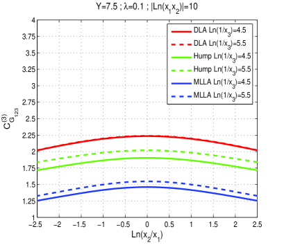
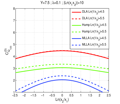
Refer to caption
Refer to caption
Figure 3: Three-particle correlations inside a gluon jet (left) and a quark jet (right) as a function of 12=ln(x2/x1)subscript1subscript2subscript𝑥2subscript𝑥1\ell_{1}-\ell_{2}=\ln(x_{2}/x_{1}) for 1+2=|ln(x1x2)|=10subscript1subscript2subscript𝑥1subscript𝑥210\ell_{1}+\ell_{2}=|\ln(x_{1}x_{2})|=10, 3=ln(1/x3)=4.5, 5.5formulae-sequencesubscript31subscript𝑥34.55.5\ell_{3}=\ln(1/x_{3})=4.5,\,5.5, fixed Y=7.5𝑌7.5Y=7.5 in the limiting spectrum approximation λ0𝜆0\lambda\approx 0.

From Fig.3, the correlation are observed to be the strongest when particles have the same energy xi=xjsubscript𝑥𝑖subscript𝑥𝑗x_{i}=x_{j} for fixed xksubscript𝑥𝑘x_{k} and to decrease when one parton is much harder the others. Indeed, in this region of the phase space two competing effects should be satisfied: on one hand, as a consequence of gluon coherence and AO, gluon emission angles should decrease and on the other hand, the convergence of the perturbative series k=xiEΘiQ0subscript𝑘perpendicular-tosubscript𝑥𝑖𝐸subscriptΘ𝑖subscript𝑄0k_{\perp}=x_{i}E\Theta_{i}\geq Q_{0} should be guaranteed. That is why, as the collinear cut-off parameter Q0subscript𝑄0Q_{0} is reached, gluons are emitted at larger angles and destructive interferences with previous emissions occur. Moreover, the observable increases for softer partons with x3subscript𝑥3x_{3} decreasing, which is for partons less sensitive to the energy balance. In Fig.4 the MLLA correlations increase for softer partons, then flatten and decrease as a consequence of soft gluon coherence, reproducing for three-particle correlations, the hump-backed shape of the one-particle distribution. Because of the limitation of the phase space, one has 𝒞(3)1superscript𝒞31{\cal C}^{(3)}\leq 1 for harder partons. Finally, in Fig.5, we display the three-particle correlators as function of the sum |ln(x1x2x3)|subscript𝑥1subscript𝑥2subscript𝑥3|\ln(x_{1}x_{2}x_{3})|, for x1=x2=x3subscript𝑥1subscript𝑥2subscript𝑥3x_{1}=x_{2}=x_{3}; when compared with Fig.4 and Fig.3, the correlators are shown to be larger. That is why, and as expected, the correlations are the strongest for particles having the same energy-momentum x1=x2=x3subscript𝑥1subscript𝑥2subscript𝑥3x_{1}=x_{2}=x_{3}. In these figures, the MLLA hump approximation is seen to become larger than the DLA correlator for smaller values of x𝑥x than those close to the hump region, which is unphysical. This is due to the fact that this approximation should not be trusted beyond the hump region Y/2σY3/2much-less-thandelimited-∣∣𝑌2𝜎proportional-tosuperscript𝑌32\mid\ell-Y/2\mid\ll\sigma\propto Y^{3/2}, 3Y/2=11.253𝑌211.253Y/2=11.25 in this case.

The MLLA hump approximation from subsection 2.7 is observed to be larger than the MLLA solution from the steepest descent of the one-particle distribution but one should bear in mind that this is only an approximation made for the sake of clarity in the interpretation of the solutions. In particular, from Fig.3 one can observe a smoother descent for the slope of the correlators in this case than that given from the more exact steepest descent. This difference comes from the role played by the iterative corrections displayed in Fig.8, which decrease the correlators away from the hump region when one of the partons becomes harder than the others. Near the maximum xi=xjsubscript𝑥𝑖subscript𝑥𝑗x_{i}=x_{j} of the correlators, the difference between the two approaches is 𝒪(k2Y2γ0)𝒪superscriptsubscript𝑘2superscript𝑌2subscript𝛾0{\cal O}\left(\frac{\ell_{k}^{2}}{Y^{2}}\gamma_{0}\right) and should decrease for xi1subscript𝑥𝑖1x_{i}\to 1, according to (80).

Refer to caption
Refer to caption
Figure 4: Three-particle correlations inside a gluon jet (left) and a quark jet (right) as a function of 1+2=|ln(x1x2)|subscript1subscript2subscript𝑥1subscript𝑥2\ell_{1}+\ell_{2}=|\ln(x_{1}x_{2})| for x1=x2subscript𝑥1subscript𝑥2x_{1}=x_{2}, 3=ln(1/x3)=4.5, 5.5formulae-sequencesubscript31subscript𝑥34.55.5\ell_{3}=\ln(1/x_{3})=4.5,\,5.5, fixed Y=7.5𝑌7.5Y=7.5 in the limiting spectrum approximation λ0𝜆0\lambda\approx 0.
Refer to caption
Refer to caption
Figure 5: Three-particle correlations inside a gluon jet (left) and a quark jet (right) as a function of 1+2+3=|ln(x1x2x3)|subscript1subscript2subscript3subscript𝑥1subscript𝑥2subscript𝑥3\ell_{1}+\ell_{2}+\ell_{3}=|\ln(x_{1}x_{2}x_{3})| for x1=x2=x3subscript𝑥1subscript𝑥2subscript𝑥3x_{1}=x_{2}=x_{3}, fixed Y=7.5𝑌7.5Y=7.5 in the limiting spectrum approximation λ0𝜆0\lambda\approx 0.

3.2 Predictions beyond the limiting spectrum 𝝀𝟎𝝀0\boldsymbol{\lambda\neq 0}
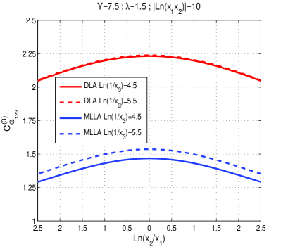
Refer to caption
Refer to caption
Figure 6: Three-particle correlations inside a gluon jet (left) and a quark jet (right) as a function of 12=ln(x2/x1)subscript1subscript2subscript𝑥2subscript𝑥1\ell_{1}-\ell_{2}=\ln(x_{2}/x_{1}) for 1+2=|ln(x1x2)|=10subscript1subscript2subscript𝑥1subscript𝑥210\ell_{1}+\ell_{2}=|\ln(x_{1}x_{2})|=10, 3=ln(1/x3)=4.5, 5.5formulae-sequencesubscript31subscript𝑥34.55.5\ell_{3}=\ln(1/x_{3})=4.5,\,5.5, fixed Y=7.5𝑌7.5Y=7.5 in the limiting spectrum approximation λ=1.5𝜆1.5\lambda=1.5.

The approximated evaluation of the one-particle distribution from the steepest descent method made possible the evaluation of the two-particle correlations beyond the limiting spectrum approximation, that is for Q0ΛQCDsubscript𝑄0subscriptΛ𝑄𝐶𝐷Q_{0}\neq\Lambda_{QCD}. Accordingly, it makes also possible the evaluation of the three-particle correlators 𝒞G123(3)(1,2,3,Y)subscriptsuperscript𝒞3subscript𝐺123subscript1subscript2subscript3𝑌{\cal C}^{(3)}_{G_{123}}(\ell_{1},\ell_{2},\ell_{3},Y) and 𝒞Q123(3)(1,2,3,Y)subscriptsuperscript𝒞3subscript𝑄123subscript1subscript2subscript3𝑌{\cal C}^{(3)}_{Q_{123}}(\ell_{1},\ell_{2},\ell_{3},Y) beyond this limit λ0𝜆0\lambda\neq 0. This parameter, also known as hadronization parameter, guarantees in particular the convergence of the perturbative approach αs1much-less-thansubscript𝛼𝑠1\alpha_{s}\ll 1. In Fig.6 and Fig.7 we display the same set of curves beyond the limiting spectrum (λ=1.5𝜆1.5\lambda=1.5) as in Fig.3 and Fig.4 in the limiting spectrum (λ0similar-to𝜆0\lambda\sim 0), with the exception of curves coming from the hump approximation. The value of λ𝜆\lambda in this case was evaluated for Q01similar-tosubscript𝑄01Q_{0}\sim 1 GeV, which corresponds to the proton mass, and ΛQCD=250subscriptΛ𝑄𝐶𝐷250\Lambda_{QCD}=250 MeV. As observed the correlation increases with λ𝜆\lambda and the range where 𝒞(3)1superscript𝒞31{\cal C}^{(3)}\geq 1 becomes larger in this case.

Refer to caption
Refer to caption
Figure 7: Three-particle correlations inside a gluon jet (left) and a quark jet (right) as a function of 1+2=|ln(x1x2)|subscript1subscript2subscript𝑥1subscript𝑥2\ell_{1}+\ell_{2}=|\ln(x_{1}x_{2})| for x1=x2subscript𝑥1subscript𝑥2x_{1}=x_{2}, 3=ln(1/x3)=4.5, 5.5formulae-sequencesubscript31subscript𝑥34.55.5\ell_{3}=\ln(1/x_{3})=4.5,\,5.5, fixed Y=7.5𝑌7.5Y=7.5 in the limiting spectrum approximation λ=1.5𝜆1.5\lambda=1.5.

4 Conclusions

In this paper we provide the first full pQCD treatment of three-particle correlations in parton showers and a further refined test of the LPHD within the limiting spectrum approximation and beyond. The evolution equations satisfied by this differential observable have been obtained for the first time and the differential version of the equations has been solved iteratively. It has been possible to interpret the analytical solution in terms of Feynman diagrams describing the process and to evaluate it from the steepest descent method applied to the single inclusive distribution. The correlations have been displayed in the range x0.014less-than-or-similar-to𝑥0.014x\lesssim 0.014, where the process is dominated by three particles emitted from the same partonic cascade following the QCD AO described in Fig.1 and Fig.2d. Furthermore, four-particle correlations have been computed at DLA so as to show that the inclusion of higher order corrections for more than three particles would rather be a cumbersome task. The correlations have been shown to be strongest for the softest hadrons having the same energy x1=x2=x3subscript𝑥1subscript𝑥2subscript𝑥3x_{1}=x_{2}=x_{3} in both quark and gluon jets, increasing as a function of ln(xi/xj)subscript𝑥𝑖subscript𝑥𝑗\ln(x_{i}/x_{j}) and |ln(xixj)|subscript𝑥𝑖subscript𝑥𝑗|\ln(x_{i}x_{j})| when xksubscript𝑥𝑘x_{k} softens, that is for partons being less sensitive to the energy balance.

Coherence effects appear when one or two of the partons involved in the process is harder than the others, thus reproducing for this observable the hump-backed shape of the one particle distribution. Away from the maximum at xi=xisubscript𝑥𝑖subscript𝑥𝑖x_{i}=x_{i}, because of limitation of the phase space, one has 𝒞(3)1superscript𝒞31{\cal C}^{(3)}\leq 1. Predictions beyond the limiting spectrum for heavier charged hadrons as compared with pions and kaons show that the correlations should increase as the parameter Q0subscript𝑄0Q_{0} equals the mass of such hadrons and the range where 𝒞(3)1superscript𝒞31{\cal C}^{(3)}\geq 1 has been enlarged beyond this limit. The last statement is not surprising because soft gluon emission gets suppressed between the two scales Q0subscript𝑄0Q_{0} and ΛQCDsubscriptΛ𝑄𝐶𝐷\Lambda_{QCD} for λ0𝜆0\lambda\neq 0, thus decreasing the particle yield inside the whole jet. This measurement would in particular provide an additional and independent check of the LPHD for massive charged hadrons. As was shown in 2.4, the DLA solution of the evolution equations provide general features of the observable showing its unreliability to be compared with the experiment. That is why, the MLLA shape and overall normalization of this observable should be compared with the data. In the case of pp¯𝑝¯𝑝p\bar{p} collisions at the Tevatron, since diet events consist of both gluon and quark jets, in order to compare data to theory, a parameter fgsubscript𝑓𝑔f_{g} for mixed samples of quark and gluon jets was chosen [11]. In pp𝑝𝑝pp collisions at the LHC, the same procedure can be applied so as to measure the two- and three-particle correlations. Furthermore, MLLA corrections have been shown to be larger for three than for two particles, that is to increase as the number of particles increases.
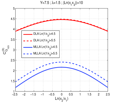
As was the case for two particles, the three-particle correlations are larger inside a quark than in a gluon jet. Same trends have been observed in HERA and LEP data for soft multi-particle fluctuations in [34, 35].

Finally, we give the first analytical predictions for intra-jet three-particle correlations in view of forthcoming measurements by ATLAS, CMS and ALICE at the LHC.

Acknowledgements

We gratefully acknowledge enlightening discussions with W. Ochs and E. Sarkisyan-Grinbau as well as support from Generalitat Valenciana under grant PROMETEO/2008/004 and M.A.S. from FPA2008-02878 and GVPROMETEO2010-056. V.M acklowledges support from the grant HadronPhysics2, a FP7-Integrating Activities and Infrastructure Program of the European Commission under Grant 227431, by UE (Feder) and the MICINN (Spain) grant FPA 2010-21750-C02-01.

Appendix A MLLA approximation

In (24a), for ln(1z)lnxmuch-less-than1𝑧𝑥\ln(1-z)\ll\ln x and lnzlnxmuch-less-than𝑧𝑥\ln z\ll\ln x, we perform the following Taylor expansions:

Q(3)(1z)Q(3)ln(1z)dQ(3)d1+𝒪(αs),superscript𝑄31𝑧superscript𝑄31𝑧𝑑superscript𝑄3𝑑subscript1𝒪subscript𝛼𝑠Q^{(3)}(1-z)-Q^{(3)}\approx\ln(1-z)\frac{dQ^{(3)}}{d\ell_{1}}+{\cal O}(\alpha_{s}), (84)
(Qij(2)(1z)Qij(2))(Gk(z)Qk)+(Gij(2)(z)Qij(2))(Qk(1z)Qk)subscriptsuperscript𝑄2𝑖𝑗1𝑧subscriptsuperscript𝑄2𝑖𝑗subscript𝐺𝑘𝑧subscript𝑄𝑘subscriptsuperscript𝐺2𝑖𝑗𝑧subscriptsuperscript𝑄2𝑖𝑗subscript𝑄𝑘1𝑧subscript𝑄𝑘\displaystyle\left(Q^{(2)}_{ij}(1-z)-Q^{(2)}_{ij}\right)(G_{k}(z)-Q_{k})+\left(G^{(2)}_{ij}(z)-Q^{(2)}_{ij}\right)\left(Q_{k}(1-z)-Q_{k}\right) (85)
=ln(1z)[dQij(2)d1(GkQk)+(Gij(2)Qij(2))dQkd1]+𝒪(αs),absent1𝑧delimited-[]𝑑subscriptsuperscript𝑄2𝑖𝑗𝑑subscript1subscript𝐺𝑘subscript𝑄𝑘subscriptsuperscript𝐺2𝑖𝑗subscriptsuperscript𝑄2𝑖𝑗𝑑subscript𝑄𝑘𝑑subscript1𝒪subscript𝛼𝑠\displaystyle=\ln(1-z)\left[\frac{dQ^{(2)}_{ij}}{d\ell_{1}}(G_{k}-Q_{k})+\left(G^{(2)}_{ij}-Q^{(2)}_{ij}\right)\frac{dQ_{k}}{d\ell_{1}}\right]+{\cal O}(\alpha_{s}), (86)
(QiGi(z))(Qj(1z)Qj)Qkln(1z)(QiGi)dQjd1Qk+𝒪(αs).subscript𝑄𝑖subscript𝐺𝑖𝑧subscript𝑄𝑗1𝑧subscript𝑄𝑗subscript𝑄𝑘1𝑧subscript𝑄𝑖subscript𝐺𝑖𝑑subscript𝑄𝑗𝑑subscript1subscript𝑄𝑘𝒪subscript𝛼𝑠\left(Q_{i}-G_{i}(z)\right)\left(Q_{j}(1-z)-Q_{j}\right)Q_{k}\approx\ln(1-z)(Q_{i}-G_{i})\frac{dQ_{j}}{d\ell_{1}}Q_{k}+{\cal O}(\alpha_{s}). (87)

Since none of these terms contribute to MLLA 𝒪(αs)𝒪subscript𝛼𝑠{\cal O}(\sqrt{\alpha_{s}}), they will be dropped hereafter. In equation (24g), we perform the following approximations in the hard fragmentation region,

(Gij(2)(z)Gij(2))(Gk(1z)Gk)lnzln(1z)dGij(2)d1Gkd1+𝒪(αs),subscriptsuperscript𝐺2𝑖𝑗𝑧subscriptsuperscript𝐺2𝑖𝑗subscript𝐺𝑘1𝑧subscript𝐺𝑘𝑧1𝑧𝑑subscriptsuperscript𝐺2𝑖𝑗𝑑subscript1subscript𝐺𝑘𝑑subscript1𝒪subscript𝛼𝑠\left(G^{(2)}_{ij}(z)-G^{(2)}_{ij}\right)\left(G_{k}(1-z)-G_{k}\right)\approx\ln z\ln(1-z)\frac{dG^{(2)}_{ij}}{d\ell_{1}}\frac{G_{k}}{d\ell_{1}}+{\cal O}(\alpha_{s}), (88)
(GiGi(z))(Gj(1z)Gj)Gklnzln(1z)dGid1dGjd1Gk+𝒪(αs).subscript𝐺𝑖subscript𝐺𝑖𝑧subscript𝐺𝑗1𝑧subscript𝐺𝑗subscript𝐺𝑘𝑧1𝑧𝑑subscript𝐺𝑖𝑑subscript1𝑑subscript𝐺𝑗𝑑subscript1subscript𝐺𝑘𝒪subscript𝛼𝑠(G_{i}-G_{i}(z))(G_{j}(1-z)-G_{j})G_{k}\approx-\ln z\ln(1-z)\frac{dG_{i}}{d\ell_{1}}\frac{dG_{j}}{d\ell_{1}}G_{k}+{\cal O}(\alpha_{s}). (89)

Neither (88) nor (89) contribute to MLLA. The other terms in (24g) can be written as,

2Q(3)(z)G(3)(2Q(3)G(3))+2lnzdQ(3)d1+𝒪(αs)2superscript𝑄3𝑧superscript𝐺32superscript𝑄3superscript𝐺32𝑧𝑑superscript𝑄3𝑑subscript1𝒪subscript𝛼𝑠2Q^{(3)}(z)-G^{(3)}\approx(2Q^{(3)}-G^{(3)})+2\ln z\frac{dQ^{(3)}}{d\ell_{1}}+{\cal O}(\alpha_{s}) (90)
2(Qij(2)(z)Gij(2))(Qk(1z)Gk)2(Qij(2)Gij(2))(QkGk)2subscriptsuperscript𝑄2𝑖𝑗𝑧subscriptsuperscript𝐺2𝑖𝑗subscript𝑄𝑘1𝑧subscript𝐺𝑘2subscriptsuperscript𝑄2𝑖𝑗subscriptsuperscript𝐺2𝑖𝑗subscript𝑄𝑘subscript𝐺𝑘\displaystyle 2\left(Q^{(2)}_{ij}(z)-G^{(2)}_{ij}\right)(Q_{k}(1-z)-G_{k})\approx 2\left(Q^{(2)}_{ij}-G^{(2)}_{ij}\right)(Q_{k}-G_{k}) (91)
+2ln(1z)(Qij(2)Gij(2))dQkd1+2lnz(QkGk)dQij(2)d1+𝒪(αs),21𝑧subscriptsuperscript𝑄2𝑖𝑗subscriptsuperscript𝐺2𝑖𝑗𝑑subscript𝑄𝑘𝑑subscript12𝑧subscript𝑄𝑘subscript𝐺𝑘𝑑subscriptsuperscript𝑄2𝑖𝑗𝑑subscript1𝒪subscript𝛼𝑠\displaystyle+2\ln(1-z)\left(Q^{(2)}_{ij}-G^{(2)}_{ij}\right)\frac{dQ_{k}}{d\ell_{1}}+2\ln z(Q_{k}-G_{k})\frac{dQ^{(2)}_{ij}}{d\ell_{1}}+{\cal O}(\alpha_{s}),
(2Qi(z)Qj(z)GiGj)Gk(2QiQjGiGj)Gk+lnz(QidQjd1+dQid1Qj)+𝒪(αs),2subscript𝑄𝑖𝑧subscript𝑄𝑗𝑧subscript𝐺𝑖subscript𝐺𝑗subscript𝐺𝑘2subscript𝑄𝑖subscript𝑄𝑗subscript𝐺𝑖subscript𝐺𝑗subscript𝐺𝑘𝑧subscript𝑄𝑖𝑑subscript𝑄𝑗𝑑subscript1𝑑subscript𝑄𝑖𝑑subscript1subscript𝑄𝑗𝒪subscript𝛼𝑠(2Q_{i}(z)Q_{j}(z)-G_{i}G_{j})G_{k}\approx(2Q_{i}Q_{j}-G_{i}G_{j})G_{k}+\ln z\left(Q_{i}\frac{dQ_{j}}{d\ell_{1}}+\frac{dQ_{i}}{d\ell_{1}}Q_{j}\right)+{\cal O}(\alpha_{s}), (92)
(Gi2Qi(z))(2Qj(1z)Gj)Gksubscript𝐺𝑖2subscript𝑄𝑖𝑧2subscript𝑄𝑗1𝑧subscript𝐺𝑗subscript𝐺𝑘\displaystyle(G_{i}-2Q_{i}(z))(2Q_{j}(1-z)-G_{j})G_{k}\!\! \displaystyle\!\!\approx\!\! (Gi2Qi)(2QjGj)Gk2(2QjGj)GklnzdQid1Gksubscript𝐺𝑖2subscript𝑄𝑖2subscript𝑄𝑗subscript𝐺𝑗subscript𝐺𝑘22subscript𝑄𝑗subscript𝐺𝑗subscript𝐺𝑘𝑧𝑑subscript𝑄𝑖𝑑subscript1subscript𝐺𝑘\displaystyle\!\!(G_{i}-2Q_{i})(2Q_{j}-G_{j})G_{k}-2(2Q_{j}-G_{j})G_{k}\ln z\frac{dQ_{i}}{d\ell_{1}}G_{k} (93)
+\displaystyle\!\!+\!\! 2(Gi2Qi)ln(1z)dQjd1Gk+𝒪(αs),2subscript𝐺𝑖2subscript𝑄𝑖1𝑧𝑑subscript𝑄𝑗𝑑subscript1subscript𝐺𝑘𝒪subscript𝛼𝑠\displaystyle\!\!2(G_{i}-2Q_{i})\ln(1-z)\frac{dQ_{j}}{d\ell_{1}}G_{k}+{\cal O}(\alpha_{s}), (94)

such that only the first terms in (90), (91), (92) and (94) will be kept in the following. Furthermore, we make use of the identity [19]

1𝑑zΦgg(z)(G(3)(z)zG(3))=1𝑑z(1z)Φgg(z)(G(3)(z)+(G(3)(z)G(3))),superscript1differential-d𝑧superscriptsubscriptΦ𝑔𝑔𝑧superscript𝐺3𝑧𝑧superscript𝐺3superscript1differential-d𝑧1𝑧superscriptsubscriptΦ𝑔𝑔𝑧superscript𝐺3𝑧superscript𝐺3𝑧superscript𝐺3\int^{1}dz\Phi_{g}^{g}(z)\left(G^{(3)}(z)-zG^{(3)}\right)=\int^{1}dz(1-z)\Phi_{g}^{g}(z)\left(G^{(3)}(z)+\left(G^{(3)}(z)-G^{(3)}\right)\right),

such that G(n)(z)zG(n)superscript𝐺𝑛𝑧𝑧superscript𝐺𝑛G^{(n)}(z)-zG^{(n)} can be replaced by,

G(n)(z)zG(n)(1z)[G(n)(z)+(G(n)(z)G(n))](1z)[G(n)(z)+lnzdG(n)d1],superscript𝐺𝑛𝑧𝑧superscript𝐺𝑛1𝑧delimited-[]superscript𝐺𝑛𝑧superscript𝐺𝑛𝑧superscript𝐺𝑛1𝑧delimited-[]superscript𝐺𝑛𝑧𝑧𝑑superscript𝐺𝑛𝑑subscript1G^{(n)}(z)-zG^{(n)}\to(1-z)\left[G^{(n)}(z)+\left(G^{(n)}(z)-G^{(n)}\right)\right]\approx(1-z)\left[G^{(n)}(z)+\ln z\frac{dG^{(n)}}{d\ell_{1}}\right],

(n=1,2,3𝑛123n=1,2,3) in the r.h.s. of equations (22b), (23c) and (24g). Indeed, terms lnz,ln(1z)proportional-toabsent𝑧1𝑧\propto\ln z,\ln(1-z) provide NMLLA corrections 𝒪(αs)𝒪subscript𝛼𝑠{\cal O}(\alpha_{s}) which improve energy conservation; however, their inclusion goes beyond the scope of the present paper.

A.1 One and two particle distributions at small 𝒙𝒙\boldsymbol{x}

The MLLA integro-differential version of equations (22a,22b) and (23c,23b) is obtained after integrating over the regular part of the splitting functions, such that [6, 19, 18]

Qi,ysubscript𝑄𝑖𝑦\displaystyle Q_{i,y}\!\! =\displaystyle\!\!=\!\! CFNc0𝑑γ02(+y)Gi(,y)34CFNcγ02(+y)Gi(,y),subscript𝐶𝐹subscript𝑁𝑐superscriptsubscript0differential-dsuperscriptsuperscriptsubscript𝛾02superscript𝑦subscript𝐺𝑖superscript𝑦34subscript𝐶𝐹subscript𝑁𝑐superscriptsubscript𝛾02𝑦subscript𝐺𝑖𝑦\displaystyle\!\!\frac{C_{F}}{N_{c}}\int_{0}^{\ell}d\ell^{\prime}\gamma_{0}^{2}(\ell^{\prime}+y)G_{i}(\ell^{\prime},y)-\frac{3}{4}\frac{C_{F}}{N_{c}}\gamma_{0}^{2}(\ell+y)G_{i}(\ell,y), (95)
Gi,ysubscript𝐺𝑖𝑦\displaystyle G_{i,y}\!\! =\displaystyle\!\!=\!\! 0𝑑γ02(+y)Gi(,y)aγ02(+y)Gi(,y),superscriptsubscript0differential-dsuperscriptsuperscriptsubscript𝛾02superscript𝑦subscript𝐺𝑖superscript𝑦𝑎superscriptsubscript𝛾02𝑦subscript𝐺𝑖𝑦\displaystyle\!\!\int_{0}^{\ell}d\ell^{\prime}\gamma_{0}^{2}(\ell^{\prime}+y)G_{i}(\ell^{\prime},y)-a\gamma_{0}^{2}(\ell+y)G_{i}(\ell,y), (96)

with γ02(+y)=1β0(+y+λ)superscriptsubscript𝛾02𝑦1subscript𝛽0𝑦𝜆\gamma_{0}^{2}(\ell+y)=\frac{1}{\beta_{0}(\ell+y+\lambda)}, and the two-particle correlations (A^ij(2)=Aij(2)AiAjsubscriptsuperscript^𝐴2𝑖𝑗subscriptsuperscript𝐴2𝑖𝑗subscript𝐴𝑖subscript𝐴𝑗\hat{A}^{(2)}_{ij}=A^{(2)}_{ij}-A_{i}A_{j}) [19, 18],

Q^ij,y(2)subscriptsuperscript^𝑄2𝑖𝑗𝑦\displaystyle\hat{Q}^{(2)}_{ij,y}\!\! =\displaystyle\!\!=\!\! CFNc0i𝑑γ02(+yj)Gij(2)(,yj,ηij)34CFNcγ02(i+yj)Gij(2)(i,yj,ηij),subscript𝐶𝐹subscript𝑁𝑐superscriptsubscript0subscript𝑖differential-dsuperscriptsubscript𝛾02subscript𝑦𝑗subscriptsuperscript𝐺2𝑖𝑗subscript𝑦𝑗subscript𝜂𝑖𝑗34subscript𝐶𝐹subscript𝑁𝑐superscriptsubscript𝛾02subscript𝑖subscript𝑦𝑗subscriptsuperscript𝐺2𝑖𝑗subscript𝑖subscript𝑦𝑗subscript𝜂𝑖𝑗\displaystyle\!\!\frac{C_{F}}{N_{c}}\int_{0}^{\ell_{i}}d\ell\gamma_{0}^{2}(\ell+y_{j})G^{(2)}_{ij}(\ell,y_{j},\eta_{ij})-\frac{3}{4}\frac{C_{F}}{N_{c}}\gamma_{0}^{2}(\ell_{i}+y_{j})G^{(2)}_{ij}(\ell_{i},y_{j},\eta_{ij}), (97)
G^ij,y(2)subscriptsuperscript^𝐺2𝑖𝑗𝑦\displaystyle\hat{G}^{(2)}_{ij,y}\!\! =\displaystyle\!\!=\!\! 0iγ02(+yj)G(2)(,yj,ηij)aγ02(i+yj)Gij(2)(i,yj,ηij)superscriptsubscript0subscript𝑖superscriptsubscript𝛾02subscript𝑦𝑗superscript𝐺2subscript𝑦𝑗subscript𝜂𝑖𝑗𝑎superscriptsubscript𝛾02subscript𝑖subscript𝑦𝑗subscriptsuperscript𝐺2𝑖𝑗subscript𝑖subscript𝑦𝑗subscript𝜂𝑖𝑗\displaystyle\!\!\int_{0}^{\ell_{i}}\gamma_{0}^{2}(\ell+y_{j})G^{(2)}(\ell,y_{j},\eta_{ij})-a\gamma_{0}^{2}(\ell_{i}+y_{j})G^{(2)}_{ij}(\ell_{i},y_{j},\eta_{ij}) (98)
+\displaystyle\!\!+\!\! (ab)γ02(i+yj)G(i,yj+ηij)G(i+ηij,yj),𝑎𝑏superscriptsubscript𝛾02subscript𝑖subscript𝑦𝑗𝐺subscript𝑖subscript𝑦𝑗subscript𝜂𝑖𝑗𝐺subscript𝑖subscript𝜂𝑖𝑗subscript𝑦𝑗\displaystyle\!\!(a-b)\gamma_{0}^{2}(\ell_{i}+y_{j})G(\ell_{i},y_{j}+\eta_{ij})G(\ell_{i}+\eta_{ij},y_{j}), (99)

with γ02(i+yj)=1β0(i+yj+ηij+λ)superscriptsubscript𝛾02subscript𝑖subscript𝑦𝑗1subscript𝛽0subscript𝑖subscript𝑦𝑗subscript𝜂𝑖𝑗𝜆\gamma_{0}^{2}(\ell_{i}+y_{j})=\frac{1}{\beta_{0}(\ell_{i}+y_{j}+\eta_{ij}+\lambda)}, after accounting for hard corrections 𝒪(αs)𝒪subscript𝛼𝑠{\cal O}(\sqrt{\alpha_{s}}). After differentiating (95,96) and (97,98) with respect to ``"``"``\ell", one has [19]

Qi,ysubscript𝑄𝑖𝑦\displaystyle Q_{i,\ell y}\!\! =\displaystyle\!\!=\!\! CFNcγ02GiCFNc34γ02(Gi,β0γ02Gi),subscript𝐶𝐹subscript𝑁𝑐superscriptsubscript𝛾02subscript𝐺𝑖subscript𝐶𝐹subscript𝑁𝑐34superscriptsubscript𝛾02subscript𝐺𝑖subscript𝛽0superscriptsubscript𝛾02subscript𝐺𝑖\displaystyle\!\!\frac{C_{F}}{N_{c}}\gamma_{0}^{2}G_{i}-\frac{C_{F}}{N_{c}}\frac{3}{4}\gamma_{0}^{2}(G_{i,\ell}-\beta_{0}\gamma_{0}^{2}G_{i}), (100)
Gi,ysubscript𝐺𝑖𝑦\displaystyle G_{i,\ell y}\!\! =\displaystyle\!\!=\!\! γ02Giaγ02(Gi,β0γ02Gi),superscriptsubscript𝛾02subscript𝐺𝑖𝑎superscriptsubscript𝛾02subscript𝐺𝑖subscript𝛽0superscriptsubscript𝛾02subscript𝐺𝑖\displaystyle\!\!\gamma_{0}^{2}G_{i}-a\gamma_{0}^{2}(G_{i,\ell}-\beta_{0}\gamma_{0}^{2}G_{i}), (101)

from where the following useful relations hold in MLLA [19],

Qi,yγ02Qisubscript𝑄𝑖𝑦superscriptsubscript𝛾02subscript𝑄𝑖\displaystyle\frac{Q_{i,\ell y}}{\gamma_{0}^{2}Q_{i}}\!\! =\displaystyle\!\!=\!\! [134ψi,]CFNcGiQi+𝒪(γ02),delimited-[]134subscript𝜓𝑖subscript𝐶𝐹subscript𝑁𝑐subscript𝐺𝑖subscript𝑄𝑖𝒪superscriptsubscript𝛾02\displaystyle\!\!\left[1-\frac{3}{4}\psi_{i,\ell}\right]\frac{C_{F}}{N_{c}}\frac{G_{i}}{Q_{i}}+{\cal O}(\gamma_{0}^{2}), (102)
GiQisubscript𝐺𝑖subscript𝑄𝑖\displaystyle\frac{G_{i}}{Q_{i}}\!\! =\displaystyle\!\!=\!\! NcCF[1(a34)ψi,]+𝒪(γ02),subscript𝑁𝑐subscript𝐶𝐹delimited-[]1𝑎34subscript𝜓𝑖𝒪superscriptsubscript𝛾02\displaystyle\!\!\frac{N_{c}}{C_{F}}\left[1-\left(a-\frac{3}{4}\right)\psi_{i,\ell}\right]+{\cal O}(\gamma_{0}^{2}), (103)
Qi,yγ02Qisubscript𝑄𝑖𝑦superscriptsubscript𝛾02subscript𝑄𝑖\displaystyle\frac{Q_{i,\ell y}}{\gamma_{0}^{2}Q_{i}}\!\! =\displaystyle\!\!=\!\! 1aψi,+𝒪(γ02).1𝑎subscript𝜓𝑖𝒪superscriptsubscript𝛾02\displaystyle\!\!1-a\psi_{i,\ell}+{\cal O}(\gamma_{0}^{2}). (104)

Corrections β0proportional-toabsentsubscript𝛽0\propto\beta_{0} in (100) and (101), which are NMLLA, account for the running of the coupling constant αssubscript𝛼𝑠\alpha_{s} and those 34,a,(ab)proportional-toabsent34𝑎𝑎𝑏\propto\frac{3}{4},a,(a-b) account for energy conservation in the hard parton splitting region. The MLLA gluon inclusive spectrum is given by the solution of (101) [6] and can be written in the form [14]:

Gi(,y)=2Γ(B)β00π2dτπeBαB(τ,y,),subscript𝐺𝑖𝑦2Γ𝐵subscript𝛽0superscriptsubscript0𝜋2𝑑𝜏𝜋superscript𝑒𝐵𝛼subscript𝐵𝜏𝑦G_{i}(\ell,y)=2\ \frac{\Gamma(B)}{\beta_{0}}\ \int_{0}^{\frac{\pi}{2}}\ \frac{d\tau}{\pi}\,e^{-B\alpha}\ {\cal F}_{B}(\tau,y,\ell), (105)

where the integration is performed with respect to τ𝜏\tau defined by α=12lny+iτ𝛼12𝑦𝑖𝜏\displaystyle\alpha=\frac{1}{2}\ln\frac{y}{\ell}+i\tau and with

B(τ,y,)subscript𝐵𝜏𝑦\displaystyle{\cal F}_{B}(\tau,y,\ell) =\displaystyle= [coshαyy+sinhα+yβ0αsinhα]B/2IB(2Z(τ,y,)),superscriptdelimited-[]𝛼𝑦𝑦𝛼𝑦subscript𝛽0𝛼𝛼𝐵2subscript𝐼𝐵2𝑍𝜏𝑦\displaystyle\left[\frac{\cosh\alpha-\displaystyle{\frac{y-\ell}{y+\ell}}\sinh\alpha}{\displaystyle\frac{\ell+y}{\beta_{0}}\,\frac{\alpha}{\sinh\alpha}}\right]^{B/2}I_{B}(2\sqrt{Z(\tau,y,\ell)}),
Z(τ,y,)𝑍𝜏𝑦\displaystyle Z(\tau,y,\ell) =\displaystyle= +yβ0αsinhα(coshαyy+sinhα),𝑦subscript𝛽0𝛼𝛼𝛼𝑦𝑦𝛼\displaystyle\frac{\ell+y}{\beta_{0}}\,\frac{\alpha}{\sinh\alpha}\,\left(\cosh\alpha-\frac{y-\ell}{y+\ell}\sinh\alpha\right),

B=a/β0𝐵𝑎subscript𝛽0B=a/\beta_{0} and IBsubscript𝐼𝐵I_{B} is the modified Bessel function of the first kind. The formula in (105) corresponds indeed to the so-called hump-backed plateau, which describes the energy spectrum of soft hadrons in the limiting spectrum approximation Q0=ΛQCDsubscript𝑄0subscriptΛ𝑄𝐶𝐷Q_{0}=\Lambda_{QCD} [6, 28]. This result is well known and constitutes one of the strikest predictions of pQCD. The corresponding solution of (100) for Qi(,y)subscript𝑄𝑖𝑦Q_{i}(\ell,y) can be obtained from (103) with accuracy 𝒪(αs)𝒪subscript𝛼𝑠{\cal O}(\sqrt{\alpha_{s}}). The system of differential evolution equations for two-particle correlations follows from (97) and (98), such that [19]

[Qij(2)QiQj]ysubscriptdelimited-[]subscriptsuperscript𝑄2𝑖𝑗subscript𝑄𝑖subscript𝑄𝑗𝑦\displaystyle\left[Q^{(2)}_{ij}-Q_{i}Q_{j}\right]_{\ell y}\!\! =\displaystyle\!\!=\!\! CFNcγ02Gij(2)34CFNcγ02(Gij,(2)β0γ02Gij(2)),subscript𝐶𝐹subscript𝑁𝑐superscriptsubscript𝛾02subscriptsuperscript𝐺2𝑖𝑗34subscript𝐶𝐹subscript𝑁𝑐superscriptsubscript𝛾02subscriptsuperscript𝐺2𝑖𝑗subscript𝛽0superscriptsubscript𝛾02subscriptsuperscript𝐺2𝑖𝑗\displaystyle\!\!\frac{C_{F}}{N_{c}}\gamma_{0}^{2}G^{(2)}_{ij}-\frac{3}{4}\frac{C_{F}}{N_{c}}\gamma_{0}^{2}\left(G^{(2)}_{ij,\ell}-\beta_{0}\gamma_{0}^{2}G^{(2)}_{ij}\right), (106)
[Gij(2)GiGj]ysubscriptdelimited-[]subscriptsuperscript𝐺2𝑖𝑗subscript𝐺𝑖subscript𝐺𝑗𝑦\displaystyle\left[G^{(2)}_{ij}-G_{i}G_{j}\right]_{\ell y}\!\! =\displaystyle\!\!=\!\! γ02Gij(2)aγ02(Gij,(2)β0γ02Gij(2))+(ab)γ02[(GiGj)β0γ02GiGj].superscriptsubscript𝛾02subscriptsuperscript𝐺2𝑖𝑗𝑎superscriptsubscript𝛾02subscriptsuperscript𝐺2𝑖𝑗subscript𝛽0superscriptsubscript𝛾02subscriptsuperscript𝐺2𝑖𝑗𝑎𝑏superscriptsubscript𝛾02delimited-[]subscriptsubscript𝐺𝑖subscript𝐺𝑗subscript𝛽0superscriptsubscript𝛾02subscript𝐺𝑖subscript𝐺𝑗\displaystyle\!\!\gamma_{0}^{2}G^{(2)}_{ij}\!-\!a\gamma_{0}^{2}\left(G^{(2)}_{ij,\ell}\!-\!\beta_{0}\gamma_{0}^{2}G^{(2)}_{ij}\right)\!+\!(a-b)\gamma_{0}^{2}\left[\left(G_{i}G_{j}\right)_{\ell}-\beta_{0}\gamma_{0}^{2}G_{i}G_{j}\right]. (107)

In [19], the system (97,98) was solved iteratively after replacing Gij(2)=CG,ij(2)GiGjsubscriptsuperscript𝐺2𝑖𝑗subscriptsuperscript𝐶2𝐺𝑖𝑗subscript𝐺𝑖subscript𝐺𝑗G^{(2)}_{ij}=C^{(2)}_{G,ij}G_{i}G_{j} and Qij(2)=CQ,ij(2)QiQjsubscriptsuperscript𝑄2𝑖𝑗subscriptsuperscript𝐶2𝑄𝑖𝑗subscript𝑄𝑖subscript𝑄𝑗Q^{(2)}_{ij}=C^{(2)}_{Q,ij}Q_{i}Q_{j} in (107) and (106) respectively. The MLLA solutions of (106) and (107), which are to be used in the present paper read [19]

𝒞Gij(2)1subscriptsuperscript𝒞2subscript𝐺𝑖𝑗1\displaystyle{\cal C}^{(2)}_{G_{ij}}-1\!\! =\displaystyle\!\!=\!\! 1δ1ijb(ψi,+ψj,)1+Δij+δ1ij,1superscriptsubscript𝛿1𝑖𝑗𝑏subscript𝜓𝑖subscript𝜓𝑗1subscriptΔ𝑖𝑗superscriptsubscript𝛿1𝑖𝑗\displaystyle\!\!\frac{1-\delta_{1}^{ij}-b\left(\psi_{i,\ell}+\psi_{j,\ell}\right)}{1+\Delta_{ij}+\delta_{1}^{ij}}, (108)
𝒞Qij(2)1𝒞Gij(2)1subscriptsuperscript𝒞2subscript𝑄𝑖𝑗1subscriptsuperscript𝒞2subscript𝐺𝑖𝑗1\displaystyle\frac{{\cal C}^{(2)}_{Q_{ij}}-1}{{\cal C}^{(2)}_{G_{ij}}-1}\!\! =\displaystyle\!\!=\!\! NcCF[1+(ba)(ψi,+ψj,)1+Δij2+Δij],subscript𝑁𝑐subscript𝐶𝐹delimited-[]1𝑏𝑎subscript𝜓𝑖subscript𝜓𝑗1subscriptΔ𝑖𝑗2subscriptΔ𝑖𝑗\displaystyle\!\!\frac{N_{c}}{C_{F}}\left[1+(b-a)(\psi_{i,\ell}+\psi_{j,\ell})\frac{1+\Delta_{ij}}{2+\Delta_{ij}}\right], (109)

which were evaluated by the steepest descent method over the single inclusive distribution in [25]. We have introduced the following notations and functions [19],

Δij=γ02(ψi,ψj,y+ψi,yψj,)=𝒪(1);subscriptΔ𝑖𝑗superscriptsubscript𝛾02subscript𝜓𝑖subscript𝜓𝑗𝑦subscript𝜓𝑖𝑦subscript𝜓𝑗𝒪1\displaystyle\Delta_{ij}=\gamma_{0}^{-2}\left(\psi_{i,\ell}\psi_{j,y}+\psi_{i,y}\psi_{j,\ell}\right)={\cal O}(1); (110)
χij=ln𝒞˙Gij(2)=𝒪(1),χij=χij=𝒪(γ02),χy=χijy=𝒪(γ02);formulae-sequencesuperscript𝜒𝑖𝑗superscriptsubscript˙𝒞subscript𝐺𝑖𝑗2𝒪1superscriptsubscript𝜒𝑖𝑗superscript𝜒𝑖𝑗𝒪superscriptsubscript𝛾02subscript𝜒𝑦superscript𝜒𝑖𝑗𝑦𝒪superscriptsubscript𝛾02\displaystyle\quad\chi^{ij}=\ln\dot{{\cal C}}_{G_{ij}}^{(2)}={\cal O}(1),\quad\chi_{\ell}^{ij}=\frac{\partial\chi^{ij}}{\partial\ell}={\cal O}(\gamma_{0}^{2}),\qquad\chi_{y}=\frac{\partial\chi^{ij}}{\partial y}={\cal O}(\gamma_{0}^{2}); (111)
δ1ij=γ02[χij(ψi,y+ψj,y)+χyij(ψj,+ψi,)]=𝒪(γ0),superscriptsubscript𝛿1𝑖𝑗superscriptsubscript𝛾02delimited-[]superscriptsubscript𝜒𝑖𝑗subscript𝜓𝑖𝑦subscript𝜓𝑗𝑦superscriptsubscript𝜒𝑦𝑖𝑗subscript𝜓𝑗subscript𝜓𝑖𝒪subscript𝛾0\displaystyle\delta_{1}^{ij}=\gamma_{0}^{-2}\Big{[}\chi_{\ell}^{ij}(\psi_{i,y}+\psi_{j,y})+\chi_{y}^{ij}(\psi_{j,\ell}+\psi_{i,\ell})\Big{]}={\cal O}(\gamma_{0}), (112)

where, following from (45) and (46), we have evaluated the corresponding order of magnitude of these quantities in powers of the anomalous dimension γ0αsproportional-tosubscript𝛾0subscript𝛼𝑠\gamma_{0}\propto\sqrt{\alpha_{s}}. The solution is iterative with respect to corrections χ𝜒\chi and δ1subscript𝛿1\delta_{1}, which need the prior evaluation of the DLA solution 𝒞˙Gij(2)superscriptsubscript˙𝒞subscript𝐺𝑖𝑗2\dot{{\cal C}}_{G_{ij}}^{(2)} of the equations.

Appendix B Iterative solution of the evolution equations

Let us first solve the equation (59). For the sake of simplicity, it is much easier to solve the equivalent equation:

G^y(3)superscriptsubscript^𝐺𝑦3\displaystyle\hat{G}_{\ell y}^{(3)}\!\! =\displaystyle\!\!=\!\! γ02G(3)aγ02(G(3)β0γ02G(3))+(ab)γ02{[G12(2)G3+G13(2)G2+G23(2)G1]\displaystyle\!\!\gamma_{0}^{2}G^{(3)}\!-\!a\gamma_{0}^{2}\left(G^{(3)}_{\ell}\!-\!\beta_{0}\gamma_{0}^{2}G^{(3)}\right)\!+\!(a-b)\gamma_{0}^{2}\left\{\left[G^{(2)}_{12}G_{3}+G^{(2)}_{13}G_{2}+G^{(2)}_{23}G_{1}\right]_{\ell}\right.
\displaystyle\!\!-\!\! β0γ02[G12(2)G3+G13(2)G2+G23(2)G1]}+(2a3b+c)γ02[(G1G2G3)β0γ02G1G2G3].\displaystyle\!\!\left.\beta_{0}\gamma_{0}^{2}\left[G^{(2)}_{12}G_{3}+G^{(2)}_{13}G_{2}+G^{(2)}_{23}G_{1}\right]\right\}+(2a-3b+c)\gamma_{0}^{2}\left[(G_{1}G_{2}G_{3})_{\ell}\!-\!\beta_{0}\gamma_{0}^{2}G_{1}G_{2}G_{3}\right].

One has to substitute the following in the l.h.s. of the equation (B):

G(3)=𝒞G123(3)G1G2G3,Gij(2)=𝒞Gij(2)GiGj.formulae-sequencesuperscript𝐺3subscriptsuperscript𝒞3subscript𝐺123subscript𝐺1subscript𝐺2subscript𝐺3subscriptsuperscript𝐺2𝑖𝑗subscriptsuperscript𝒞2subscript𝐺𝑖𝑗subscript𝐺𝑖subscript𝐺𝑗G^{(3)}={\cal C}^{(3)}_{G_{123}}G_{1}G_{2}G_{3},\quad G^{(2)}_{ij}={\cal C}^{(2)}_{G_{ij}}G_{i}G_{j}.

Thus, after normalizing by γ02G1G2G3superscriptsubscript𝛾02subscript𝐺1subscript𝐺2subscript𝐺3\gamma_{0}^{2}G_{1}G_{2}G_{3}, one finds,

[(𝒞G123(3)1)G1G2G3]yγ02G1G2G3subscriptdelimited-[]subscriptsuperscript𝒞3subscript𝐺1231subscript𝐺1subscript𝐺2subscript𝐺3𝑦superscriptsubscript𝛾02subscript𝐺1subscript𝐺2subscript𝐺3\displaystyle\frac{\left[({\cal C}^{(3)}_{G_{123}}-1)G_{1}G_{2}G_{3}\right]_{\ell y}}{\gamma_{0}^{2}G_{1}G_{2}G_{3}}\!\! =\displaystyle\!\!=\!\! 𝒞G123(3)(ϵ1+ϵ2)+(𝒞G123(3)1)[3+Δ12+Δ13+Δ23\displaystyle\!\!{\cal C}^{(3)}_{G_{123}}(\epsilon_{1}+\epsilon_{2})+({\cal C}^{(3)}_{G_{123}}-1)\left[3+\Delta_{12}+\Delta_{13}+\Delta_{23}\right.
\displaystyle\!\!-\!\! a(ψ1,+ψ2,+ψ3,)+3aβ0γ02],\displaystyle\!\!\left.a(\psi_{1,\ell}+\psi_{2,\ell}+\psi_{3,\ell})+3a\beta_{0}\gamma_{0}^{2}\right],

while for the other terms in the r.h.s. of the same equation one finds,

[(𝒞Gij(2)1)G1G2G3]yγ02G1G2G3subscriptdelimited-[]subscriptsuperscript𝒞2subscript𝐺𝑖𝑗1subscript𝐺1subscript𝐺2subscript𝐺3𝑦superscriptsubscript𝛾02subscript𝐺1subscript𝐺2subscript𝐺3\displaystyle\frac{\left[({\cal C}^{(2)}_{G_{ij}}-1)G_{1}G_{2}G_{3}\right]_{\ell y}}{\gamma_{0}^{2}G_{1}G_{2}G_{3}}\!\! =\displaystyle\!\!=\!\! (𝒞Gij(2)1)(i=13Gi,yγ02Gi+Δ12+Δ13+Δ23)+𝒞Gij(2)ξ1ij+𝒞Gij(2)δ2ijsubscriptsuperscript𝒞2subscript𝐺𝑖𝑗1superscriptsubscript𝑖13subscript𝐺𝑖𝑦superscriptsubscript𝛾02subscript𝐺𝑖subscriptΔ12subscriptΔ13subscriptΔ23subscriptsuperscript𝒞2subscript𝐺𝑖𝑗superscriptsubscript𝜉1𝑖𝑗subscriptsuperscript𝒞2subscript𝐺𝑖𝑗superscriptsubscript𝛿2𝑖𝑗\displaystyle\!\!({\cal C}^{(2)}_{G_{ij}}-1)\!\left(\!\sum_{i=1}^{3}\frac{G_{i,\ell y}}{\gamma_{0}^{2}G_{i}}+\Delta_{12}+\Delta_{13}+\Delta_{23}\right)\!\!+{\cal C}^{(2)}_{G_{ij}}\xi_{1}^{ij}+{\cal C}^{(2)}_{G_{ij}}\delta_{2}^{ij} (115)
=\displaystyle\!\!=\!\! (𝒞Gij(2)1)[3+Δ12+Δ13+Δ23a(ψ1,+ψ2,+ψ3,)+3aβ0γ02\displaystyle\!\!({\cal C}^{(2)}_{G_{ij}}-1)\left[3+\Delta_{12}+\Delta_{13}+\Delta_{23}-a(\psi_{1,\ell}+\psi_{2,\ell}+\psi_{3,\ell})+3a\beta_{0}\gamma_{0}^{2}\right. (116)
+\displaystyle\!\!+\!\! ξ1ij+δ2ij]+ξ1ij+δ2ij.\displaystyle\!\!\left.\xi_{1}^{ij}+\delta_{2}^{ij}\right]+\xi_{1}^{ij}+\delta_{2}^{ij}. (117)

The r.h.s. provides the following contribution

r.h.s.γ02G1G2G3\displaystyle\frac{r.h.s.}{\gamma_{0}^{2}G_{1}G_{2}G_{3}}\!\! =\displaystyle\!\!=\!\! 𝒞G123(3)a𝒞G123(3)(ψ1,+ψ2,+ψ3,+ζβ0γ02)+(ab)[𝒞G12(2)(χ12+ψ1,+ψ2,\displaystyle\!\!{\cal C}^{(3)}_{G_{123}}-a{\cal C}^{(3)}_{G_{123}}(\psi_{1,\ell}+\psi_{2,\ell}+\psi_{3,\ell}+\zeta_{\ell}-\beta_{0}\gamma_{0}^{2})+(a-b)\left[{\cal C}^{(2)}_{G_{12}}(\chi_{\ell}^{12}+\psi_{1,\ell}+\psi_{2,\ell}\right. (118)
+\displaystyle\!\!+\!\! ψ3,)+𝒞(2)G13(χ13+ψ1,+ψ2,+ψ3,)+𝒞(2)G23(χ23+ψ1,+ψ2,+ψ3,)\displaystyle\!\!\left.\psi_{3,\ell})+{\cal C}^{(2)}_{G_{13}}(\chi_{\ell}^{13}+\psi_{1,\ell}+\psi_{2,\ell}+\psi_{3,\ell})+{\cal C}^{(2)}_{G_{23}}(\chi_{\ell}^{23}+\psi_{1,\ell}+\psi_{2,\ell}+\psi_{3,\ell})\right. (119)
\displaystyle\!\!-\!\! β0γ02(𝒞G12(2)+𝒞G13(2)+𝒞G23(2))]+(3b2ac)(ψ1,+ψ2,+ψ3,β0γ02).\displaystyle\!\!\left.\beta_{0}\gamma_{0}^{2}({\cal C}^{(2)}_{G_{12}}+{\cal C}^{(2)}_{G_{13}}+{\cal C}^{(2)}_{G_{23}})\right]+(3b-2a-c)(\psi_{1,\ell}+\psi_{2,\ell}+\psi_{3,\ell}-\beta_{0}\gamma_{0}^{2}). (120)

After adding (B) and (117) and equating with (120) together with some algebra in between, one finds the solution written in (61). Following the same iterative procedure

Q(3)=𝒞Q123(3)Q1Q2Q3,Qij(2)=𝒞Qij(2)QiQj;G(3)=𝒞G123(3)G1G2G3,formulae-sequencesuperscript𝑄3subscriptsuperscript𝒞3subscript𝑄123subscript𝑄1subscript𝑄2subscript𝑄3formulae-sequencesubscriptsuperscript𝑄2𝑖𝑗subscriptsuperscript𝒞2subscript𝑄𝑖𝑗subscript𝑄𝑖subscript𝑄𝑗superscript𝐺3subscriptsuperscript𝒞3subscript𝐺123subscript𝐺1subscript𝐺2subscript𝐺3Q^{(3)}={\cal C}^{(3)}_{Q_{123}}Q_{1}Q_{2}Q_{3},\quad Q^{(2)}_{ij}={\cal C}^{(2)}_{Q_{ij}}Q_{i}Q_{j};\quad G^{(3)}={\cal C}^{(3)}_{G_{123}}G_{1}G_{2}G_{3},

for the quark jet evolution equation written in (58), one has,

(𝒞Q123(3)1)(Δ~12+Δ~13+Δ~23+i=13Qi,yγ02Qi+ϵ~1+ϵ~2)subscriptsuperscript𝒞3subscript𝑄1231subscript~Δ12subscript~Δ13subscript~Δ23superscriptsubscript𝑖13subscript𝑄𝑖𝑦superscriptsubscript𝛾02subscript𝑄𝑖subscript~italic-ϵ1subscript~italic-ϵ2\displaystyle\left({\cal C}^{(3)}_{Q_{123}}-1\right)\left(\tilde{\Delta}_{12}+\tilde{\Delta}_{13}+\tilde{\Delta}_{23}+\sum_{i=1}^{3}\frac{Q_{i,\ell y}}{\gamma_{0}^{2}Q_{i}}+\tilde{\epsilon}_{1}+\tilde{\epsilon}_{2}\right) (121)
(𝒞Q12(2)1)(Δ~12+Δ~13+Δ~23+i=13Qi,yγ02Qi+ξ~112+δ~212)subscriptsuperscript𝒞2subscript𝑄121subscript~Δ12subscript~Δ13subscript~Δ23superscriptsubscript𝑖13subscript𝑄𝑖𝑦superscriptsubscript𝛾02subscript𝑄𝑖superscriptsubscript~𝜉112superscriptsubscript~𝛿212\displaystyle-\left({\cal C}^{(2)}_{Q_{12}}-1\right)\left(\tilde{\Delta}_{12}+\tilde{\Delta}_{13}+\tilde{\Delta}_{23}+\sum_{i=1}^{3}\frac{Q_{i,\ell y}}{\gamma_{0}^{2}Q_{i}}+\tilde{\xi}_{1}^{12}+\tilde{\delta}_{2}^{12}\right) (122)
(𝒞Q13(2)1)(Δ~12+Δ~13+Δ~23+i=13Qi,yγ02Qi+ξ~113+δ~213)subscriptsuperscript𝒞2subscript𝑄131subscript~Δ12subscript~Δ13subscript~Δ23superscriptsubscript𝑖13subscript𝑄𝑖𝑦superscriptsubscript𝛾02subscript𝑄𝑖superscriptsubscript~𝜉113superscriptsubscript~𝛿213\displaystyle-\left({\cal C}^{(2)}_{Q_{13}}-1\right)\left(\tilde{\Delta}_{12}+\tilde{\Delta}_{13}+\tilde{\Delta}_{23}+\sum_{i=1}^{3}\frac{Q_{i,\ell y}}{\gamma_{0}^{2}Q_{i}}+\tilde{\xi}_{1}^{13}+\tilde{\delta}_{2}^{13}\right) (123)
(𝒞Q23(2)1)(Δ~12+Δ~13+Δ~23+i=13Qi,yγ02Qi+ξ~123+δ~223)subscriptsuperscript𝒞2subscript𝑄231subscript~Δ12subscript~Δ13subscript~Δ23superscriptsubscript𝑖13subscript𝑄𝑖𝑦superscriptsubscript𝛾02subscript𝑄𝑖superscriptsubscript~𝜉123superscriptsubscript~𝛿223\displaystyle-\left({\cal C}^{(2)}_{Q_{23}}-1\right)\left(\tilde{\Delta}_{12}+\tilde{\Delta}_{13}+\tilde{\Delta}_{23}+\sum_{i=1}^{3}\frac{Q_{i,\ell y}}{\gamma_{0}^{2}Q_{i}}+\tilde{\xi}_{1}^{23}+\tilde{\delta}_{2}^{23}\right) (124)
=CFNc𝒞G123(3)[134(ψ1,+ψ2,+ψ3,+ζβ0γ02)]G1G2G3Q1Q2Q3absentsubscript𝐶𝐹subscript𝑁𝑐subscriptsuperscript𝒞3subscript𝐺123delimited-[]134subscript𝜓1subscript𝜓2subscript𝜓3subscript𝜁subscript𝛽0superscriptsubscript𝛾02subscript𝐺1subscript𝐺2subscript𝐺3subscript𝑄1subscript𝑄2subscript𝑄3\displaystyle=\frac{C_{F}}{N_{c}}{\cal C}^{(3)}_{G_{123}}\left[1-\frac{3}{4}(\psi_{1,\ell}+\psi_{2,\ell}+\psi_{3,\ell}+\zeta_{\ell}-\beta_{0}\gamma_{0}^{2})\right]\frac{G_{1}G_{2}G_{3}}{Q_{1}Q_{2}Q_{3}} (125)
+(ξ~112+δ~212)+(ξ~113+δ~213)+(ξ~123+δ~223)ϵ~1ϵ~2.superscriptsubscript~𝜉112superscriptsubscript~𝛿212superscriptsubscript~𝜉113superscriptsubscript~𝛿213superscriptsubscript~𝜉123superscriptsubscript~𝛿223subscript~italic-ϵ1subscript~italic-ϵ2\displaystyle+(\tilde{\xi}_{1}^{12}+\tilde{\delta}_{2}^{12})+(\tilde{\xi}_{1}^{13}+\tilde{\delta}_{2}^{13})+(\tilde{\xi}_{1}^{23}+\tilde{\delta}_{2}^{23})-\tilde{\epsilon}_{1}-\tilde{\epsilon}_{2}.

Finally by adding and subtracting (ϵ~1+ϵ~2)subscript~italic-ϵ1subscript~italic-ϵ2(\tilde{\epsilon}_{1}+\tilde{\epsilon}_{2}) in every term (𝒞Qij(2)1)proportional-toabsentsubscriptsuperscript𝒞2subscript𝑄𝑖𝑗1\propto\left({\cal C}^{(2)}_{Q_{ij}}-1\right) in the l.h.s. of (121) one finds (65).

Appendix C Steepest descent evaluation: reminder from [25]

The evaluation of the integral representation by the steepest descent method at small x1much-less-than𝑥1x\ll 1 (or large 1much-greater-than1\ell\gg 1) and very high energy Y1much-greater-than𝑌1Y\gg 1 leads to the result,

G(,y)𝒩(μ,ν,λ)exp[2β0(+y+λλ)μνsinhμsinhν+νaβ0(μν)],𝐺𝑦𝒩𝜇𝜈𝜆2subscript𝛽0𝑦𝜆𝜆𝜇𝜈𝜇𝜈𝜈𝑎subscript𝛽0𝜇𝜈G(\ell,y)\approx{\cal N}(\mu,\nu,\lambda)\exp\left[\frac{2}{\beta_{0}}\left(\sqrt{\ell+y+\lambda}-\sqrt{\lambda}\right)\frac{\mu-\nu}{\sinh\mu-\sinh\nu}+\nu-\frac{a}{\beta_{0}}(\mu-\nu)\right], (126)

where

𝒩(μ,ν,λ)=12(+y+λ)(β0λ)1/4πcoshνDetA(μ,ν),𝒩𝜇𝜈𝜆12𝑦𝜆superscriptsubscript𝛽0𝜆14𝜋𝜈𝐷𝑒𝑡𝐴𝜇𝜈{\cal N}(\mu,\nu,\lambda)=\frac{1}{2}(\ell+y+\lambda)\frac{\left(\frac{\beta_{0}}{\lambda}\right)^{1/4}}{\sqrt{\pi\cosh\nu DetA(\mu,\nu)}},

with

DetA(μ,ν)=β0(+y+λ)3[(μν)coshμcoshν+coshμsinhνsinhμsinhνsinh3μcoshν].𝐷𝑒𝑡𝐴𝜇𝜈subscript𝛽0superscript𝑦𝜆3delimited-[]𝜇𝜈𝜇𝜈𝜇𝜈𝜇𝜈superscript3𝜇𝜈DetA(\mu,\nu)=\beta_{0}(\ell+y+\lambda)^{3}\left[\frac{(\mu-\nu)\cosh\mu\cosh\nu+\cosh\mu\sinh\nu-\sinh\mu\sinh\nu}{\sinh^{3}\mu\cosh\nu}\right].

The logarithmic derivatives of the spectrum given in (75) and (78) were derived from (126) and it was also shown that (126) reproduces the Gaussian shape of the inclusive distribution near the hump maxY/2subscript𝑚𝑎𝑥𝑌2\ell_{max}\approx Y/2. From (126), one has indeed,

G(,y)(3πβ0[(+y+λ)3/2λ3/2])1/2exp(2β03(+y+λ)3/2λ3/2(Y/2)22),𝐺𝑦superscript3𝜋subscript𝛽0delimited-[]superscript𝑦𝜆32superscript𝜆32122subscript𝛽03superscript𝑦𝜆32superscript𝜆32superscript𝑌222G(\ell,y)\approx\left(\frac{3}{\pi\sqrt{\beta_{0}}[(\ell+y+\lambda)^{3/2}-\lambda^{3/2}]}\right)^{1/2}\exp\left(-\frac{2}{\sqrt{\beta_{0}}}\frac{3}{(\ell+y+\lambda)^{3/2}-\lambda^{3/2}}\frac{(\ell-Y/2)^{2}}{2}\right), (127)

where the MLLA maxsubscript𝑚𝑎𝑥\ell_{max} reads,

maxY2+12aβ0(Y+λλ).subscript𝑚𝑎𝑥𝑌212𝑎subscript𝛽0𝑌𝜆𝜆\ell_{max}\approx\frac{Y}{2}+\frac{1}{2}\frac{a}{\beta_{0}}\left(\sqrt{Y+\lambda}-\sqrt{\lambda}\right).

Setting a=0𝑎0a=0 and λ=0𝜆0\lambda=0 in the previous expressions one recovers the DLA results, which are needed for subsection 2.4. The functions entering as a function of (μ,ν𝜇𝜈\mu,\nu) in (75) and (78) are the following,

Q~(μ,ν)~𝑄𝜇𝜈\displaystyle\tilde{Q}(\mu,\nu)\!\! =\displaystyle\!\!=\!\! coshμsinhμcoshν(μν)coshνsinhν(μν)coshμcoshν+coshμsinhνsinhμcoshν,𝜇𝜇𝜈𝜇𝜈𝜈𝜈𝜇𝜈𝜇𝜈𝜇𝜈𝜇𝜈\displaystyle\!\!\frac{\cosh\mu\sinh\mu\cosh\nu-(\mu-\nu)\cosh\nu-\sinh\nu}{(\mu-\nu)\cosh\mu\cosh\nu+\cosh\mu\sinh\nu-\sinh\mu\cosh\nu}, (128)
K(μ,ν)𝐾𝜇𝜈\displaystyle K(\mu,\nu)\!\! =\displaystyle\!\!=\!\! 12sinhν(μν)coshμsinhμ(μν)coshμcoshν+coshμsinhνsinhμcoshν,12𝜈𝜇𝜈𝜇𝜇𝜇𝜈𝜇𝜈𝜇𝜈𝜇𝜈\displaystyle\!\!-\frac{1}{2}\sinh\nu\frac{(\mu-\nu)\cosh\mu-\sinh\mu}{(\mu-\nu)\cosh\mu\cosh\nu+\cosh\mu\sinh\nu-\sinh\mu\cosh\nu}, (129)
L(μ,ν)𝐿𝜇𝜈\displaystyle L(\mu,\nu)\!\! =\displaystyle\!\!=\!\! 32cothμ12(μν)coshνsinhμ+sinhνsinhμ(μν)coshμcoshν+coshμsinhνsinhμcoshν,32hyperbolic-cotangent𝜇12𝜇𝜈𝜈𝜇𝜈𝜇𝜇𝜈𝜇𝜈𝜇𝜈𝜇𝜈\displaystyle\!\!\frac{3}{2}\coth\mu-\frac{1}{2}\frac{(\mu-\nu)\cosh\nu\sinh\mu+\sinh\nu\sinh\mu}{(\mu-\nu)\cosh\mu\cosh\nu+\cosh\mu\sinh\nu-\sinh\mu\cosh\nu}, (130)
C(μ,ν)𝐶𝜇𝜈\displaystyle C(\mu,\nu)\!\! =\displaystyle\!\!=\!\! L(μ,ν)+tanhνcothμ(1+K(μ,ν)).𝐿𝜇𝜈𝜈hyperbolic-cotangent𝜇1𝐾𝜇𝜈\displaystyle\!\!L(\mu,\nu)+\tanh\nu\coth\mu\left(1+K(\mu,\nu)\right). (131)

The expressions for the two particle correlations follow from (108) and (109) [25],

𝒞Gij(2)superscriptsubscript𝒞subscript𝐺𝑖𝑗2\displaystyle{\cal C}_{G_{ij}}^{(2)}\!\! =\displaystyle\!\!=\!\! 1+1bγ0(eμi+eμj)δ1ij1+2cosh(μiμj)+Δ(μi,νi,μj,νj)+δ1ij,11𝑏subscript𝛾0superscript𝑒subscript𝜇𝑖superscript𝑒subscript𝜇𝑗superscriptsubscript𝛿1𝑖𝑗12subscript𝜇𝑖subscript𝜇𝑗superscriptΔsubscript𝜇𝑖subscript𝜈𝑖subscript𝜇𝑗subscript𝜈𝑗superscriptsubscript𝛿1𝑖𝑗\displaystyle\!\!1+\frac{1-b\gamma_{0}(e^{\mu_{i}}+e^{\mu_{j}})-\delta_{1}^{ij}}{1+2\cosh(\mu_{i}-\mu_{j})+\Delta^{\prime}(\mu_{i},\nu_{i},\mu_{j},\nu_{j})+\delta_{1}^{ij}}, (132)
𝒞Qij(2)superscriptsubscript𝒞subscript𝑄𝑖𝑗2\displaystyle{\cal C}_{Q_{ij}}^{(2)}\!\! =\displaystyle\!\!=\!\! 1+NcCF[𝒞Gij(2)1+12(ba)γ0eμi+eμj1+cosh(μiμj)],1subscript𝑁𝑐subscript𝐶𝐹delimited-[]superscriptsubscript𝒞subscript𝐺𝑖𝑗2112𝑏𝑎subscript𝛾0superscript𝑒subscript𝜇𝑖superscript𝑒subscript𝜇𝑗1subscript𝜇𝑖subscript𝜇𝑗\displaystyle\!\!1+\frac{N_{c}}{C_{F}}\left[{\cal C}_{G_{ij}}^{(2)}-1+\frac{1}{2}(b-a)\gamma_{0}\frac{e^{\mu_{i}}+e^{\mu_{j}}}{1+\cosh(\mu_{i}-\mu_{j})}\right], (133)

where,

δ1ij=β0γ02sinh2(μiμj2)3+4sinh2(μiμj2)(Q~(μi,νi)+Q~(μj,νj)),superscriptsubscript𝛿1𝑖𝑗subscript𝛽0subscript𝛾02superscript2subscript𝜇𝑖subscript𝜇𝑗234superscript2subscript𝜇𝑖subscript𝜇𝑗2~𝑄subscript𝜇𝑖subscript𝜈𝑖~𝑄subscript𝜇𝑗subscript𝜈𝑗\delta_{1}^{ij}=\beta_{0}\gamma_{0}\frac{2\sinh^{2}\left(\frac{\mu_{i}-\mu_{j}}{2}\right)}{3+4\sinh^{2}\left(\frac{\mu_{i}-\mu_{j}}{2}\right)}\Big{(}\tilde{Q}(\mu_{i},\nu_{i})+\tilde{Q}(\mu_{j},\nu_{j})\Big{)}, (134)

and

Δ(μi,νi,μj,νj)superscriptΔsubscript𝜇𝑖subscript𝜈𝑖subscript𝜇𝑗subscript𝜈𝑗\displaystyle\Delta^{\prime}(\mu_{i},\nu_{i},\mu_{j},\nu_{j})\!\! =\displaystyle\!\!=\!\! aγ0[eμi+eμjsinh(μiμj)(Q~iQ~j)+coshμ1tanhν2+coshμ2tanhν1\displaystyle\!\!-a\gamma_{0}\left[e^{\mu_{i}}+e^{\mu_{j}}-\sinh(\mu_{i}-\mu_{j})(\tilde{Q}_{i}-\tilde{Q}_{j})+\cosh\mu_{1}\tanh\nu_{2}+\cosh\mu_{2}\tanh\nu_{1}\right. (135)
\displaystyle\!\!-\!\! sinhμitanhνjcothμjsinhμjtanhνicothμisubscript𝜇𝑖subscript𝜈𝑗hyperbolic-cotangentsubscript𝜇𝑗subscript𝜇𝑗subscript𝜈𝑖hyperbolic-cotangentsubscript𝜇𝑖\displaystyle\!\!\left.\sinh\mu_{i}\tanh\nu_{j}\coth\mu_{j}-\sinh\mu_{j}\tanh\nu_{i}\coth\mu_{i}\right. (136)
+\displaystyle\!\!+\!\! sinh(μiμj)(tanhνicothμiQ~itanhνjcothμjQ~j)]\displaystyle\!\!\left.\sinh(\mu_{i}-\mu_{j})\Big{(}\tanh\nu_{i}\coth\mu_{i}\tilde{Q}_{i}-\tanh\nu_{j}\coth\mu_{j}\tilde{Q}_{j}\Big{)}\right] (137)
\displaystyle\!\!-\!\! β0γ0[coshμisinhμiCj+coshμjsinhμjCi+sinh(μiμj)(CiQ~iCjQ~j)\displaystyle\!\!\beta_{0}\gamma_{0}\!\left[\cosh\mu_{i}-\sinh\mu_{i}C_{j}+\cosh\mu_{j}-\sinh\mu_{j}C_{i}+\sinh(\mu_{i}-\mu_{j})(C_{i}\tilde{Q}_{i}-C_{j}\tilde{Q}_{j})\right. (138)
+\displaystyle\!\!+\!\! coshμitanhνj(1+Kj)+coshμjtanhνi(1+Ki)].\displaystyle\!\!\left.\cosh\mu_{i}\tanh\nu_{j}(1+K_{j})+\cosh\mu_{j}\tanh\nu_{i}(1+K_{i})\right]. (139)

The solutions (132) and (133) are the ones to be used in this paper for the evaluations of the three-particle correlations and will be directly inserted in the solutions (61) and (65) respectively.

C.1 Corrections 𝝃𝟏𝒊𝒋,𝝃~𝟏𝒊𝒋superscriptsubscript𝝃1𝒊𝒋superscriptsubscriptbold-~𝝃1𝒊𝒋\boldsymbol{\xi_{1}^{ij}},\boldsymbol{\tilde{\xi}_{1}^{ij}} and ϵ𝟏,ϵ~𝟏subscriptbold-italic-ϵ1subscriptbold-~bold-italic-ϵ1\boldsymbol{\epsilon_{1}},\boldsymbol{\tilde{\epsilon}_{1}}

For the computation of these corrections, one only needs to take the DLA part of the logarithmic derivatives of the one-particle distribution ψi,=γ0eμisubscript𝜓𝑖subscript𝛾0superscript𝑒subscript𝜇𝑖\psi_{i,\ell}=\gamma_{0}e^{\mu_{i}} and ψi,y=γ0eμisubscript𝜓𝑖𝑦subscript𝛾0superscript𝑒subscript𝜇𝑖\psi_{i,y}=\gamma_{0}e^{-\mu_{i}}, such that after replacement in (64c) and (68c) one finds,

ξ1ijsuperscriptsubscript𝜉1𝑖𝑗\displaystyle\xi_{1}^{ij} =\displaystyle= 1γ0[χij(eμ1+eμ2+eμ3)+χyij(eμ1+eμ2+eμ3)],1subscript𝛾0delimited-[]superscriptsubscript𝜒𝑖𝑗superscript𝑒subscript𝜇1superscript𝑒subscript𝜇2superscript𝑒subscript𝜇3superscriptsubscript𝜒𝑦𝑖𝑗superscript𝑒subscript𝜇1superscript𝑒subscript𝜇2superscript𝑒subscript𝜇3\displaystyle\frac{1}{\gamma_{0}}\left[\chi_{\ell}^{ij}\left(e^{-\mu_{1}}+e^{-\mu_{2}}+e^{-\mu_{3}}\right)+\chi_{y}^{ij}\left(e^{\mu_{1}}+e^{\mu_{2}}+e^{\mu_{3}}\right)\right], (140)
ξ~1ijsuperscriptsubscript~𝜉1𝑖𝑗\displaystyle\tilde{\xi}_{1}^{ij} =\displaystyle= 1γ0[χ~ij(eμ1+eμ2+eμ3)+χ~yij(eμ1+eμ2+eμ3)],1subscript𝛾0delimited-[]superscriptsubscript~𝜒𝑖𝑗superscript𝑒subscript𝜇1superscript𝑒subscript𝜇2superscript𝑒subscript𝜇3superscriptsubscript~𝜒𝑦𝑖𝑗superscript𝑒subscript𝜇1superscript𝑒subscript𝜇2superscript𝑒subscript𝜇3\displaystyle\frac{1}{\gamma_{0}}\left[\tilde{\chi}_{\ell}^{ij}\left(e^{-\mu_{1}}+e^{-\mu_{2}}+e^{-\mu_{3}}\right)+\tilde{\chi}_{y}^{ij}\left(e^{\mu_{1}}+e^{\mu_{2}}+e^{\mu_{3}}\right)\right], (141)

where

χij=β0γ02tanhμiμj21+2cosh(μiμj)eμiQ~ieμjQ~j2,χ~ij=NcCF𝒞˙Gij(2)𝒞˙Qij(2)χij,formulae-sequencesuperscriptsubscript𝜒𝑖𝑗subscript𝛽0superscriptsubscript𝛾02subscript𝜇𝑖subscript𝜇𝑗212subscript𝜇𝑖subscript𝜇𝑗superscript𝑒subscript𝜇𝑖subscript~𝑄𝑖superscript𝑒subscript𝜇𝑗subscript~𝑄𝑗2superscriptsubscript~𝜒𝑖𝑗subscript𝑁𝑐subscript𝐶𝐹superscriptsubscript˙𝒞subscript𝐺𝑖𝑗2superscriptsubscript˙𝒞subscript𝑄𝑖𝑗2superscriptsubscript𝜒𝑖𝑗\chi_{\ell}^{ij}=\beta_{0}\gamma_{0}^{2}\frac{\tanh\frac{\mu_{i}-\mu_{j}}{2}}{1+2\cosh(\mu_{i}-\mu_{j})}\frac{e^{\mu_{i}}\tilde{Q}_{i}-e^{\mu_{j}}\tilde{Q}_{j}}{2},\quad\tilde{\chi}_{\ell}^{ij}=-\frac{N_{c}}{C_{F}}\frac{\dot{{\cal C}}_{G_{ij}}^{(2)}}{\dot{{\cal C}}_{Q_{ij}}^{(2)}}\chi_{\ell}^{ij}, (142)
χyij=β0γ02tanhμiμj21+2cosh(μiμj)eμiQ~ieμjQ~j2,χ~yij=NcCF𝒞˙Gij(2)𝒞˙Qij(2)χyij;formulae-sequencesuperscriptsubscript𝜒𝑦𝑖𝑗subscript𝛽0superscriptsubscript𝛾02subscript𝜇𝑖subscript𝜇𝑗212subscript𝜇𝑖subscript𝜇𝑗superscript𝑒subscript𝜇𝑖subscript~𝑄𝑖superscript𝑒subscript𝜇𝑗subscript~𝑄𝑗2superscriptsubscript~𝜒𝑦𝑖𝑗subscript𝑁𝑐subscript𝐶𝐹superscriptsubscript˙𝒞subscript𝐺𝑖𝑗2superscriptsubscript˙𝒞subscript𝑄𝑖𝑗2superscriptsubscript𝜒𝑦𝑖𝑗\chi_{y}^{ij}=-\beta_{0}\gamma_{0}^{2}\frac{\tanh\frac{\mu_{i}-\mu_{j}}{2}}{1+2\cosh(\mu_{i}-\mu_{j})}\frac{e^{-\mu_{i}}\tilde{Q}_{i}-e^{-\mu_{j}}\tilde{Q}_{j}}{2},\quad\tilde{\chi}_{y}^{ij}=-\frac{N_{c}}{C_{F}}\frac{\dot{{\cal C}}_{G_{ij}}^{(2)}}{\dot{{\cal C}}_{Q_{ij}}^{(2)}}\chi_{y}^{ij}; (143)

with

𝒞˙Gij(2)=1+11+2cosh(μiμj),𝒞˙Qij(2)=1+NcCF11+2cosh(μiμj).formulae-sequencesuperscriptsubscript˙𝒞subscript𝐺𝑖𝑗21112subscript𝜇𝑖subscript𝜇𝑗superscriptsubscript˙𝒞subscript𝑄𝑖𝑗21subscript𝑁𝑐subscript𝐶𝐹112subscript𝜇𝑖subscript𝜇𝑗\dot{{\cal C}}_{G_{ij}}^{(2)}=1+\frac{1}{1+2\cosh(\mu_{i}-\mu_{j})},\quad\dot{{\cal C}}_{Q_{ij}}^{(2)}=1+\frac{N_{c}}{C_{F}}\frac{1}{1+2\cosh(\mu_{i}-\mu_{j})}. (144)

Accordingly, replacing ψi,=γ0eμisubscript𝜓𝑖subscript𝛾0superscript𝑒subscript𝜇𝑖\psi_{i,\ell}=\gamma_{0}e^{\mu_{i}} and ψi,y=γ0eμisubscript𝜓𝑖𝑦subscript𝛾0superscript𝑒subscript𝜇𝑖\psi_{i,y}=\gamma_{0}e^{-\mu_{i}} in (64e) and (68e), one has

ϵ1subscriptitalic-ϵ1\displaystyle\epsilon_{1}\!\! =\displaystyle\!\!=\!\! 1γ0[ζ(eμ1+eμ2+eμ3)+ζy(eμ1+eμ2+eμ3)],1subscript𝛾0delimited-[]subscript𝜁superscript𝑒subscript𝜇1superscript𝑒subscript𝜇2superscript𝑒subscript𝜇3subscript𝜁𝑦superscript𝑒subscript𝜇1superscript𝑒subscript𝜇2superscript𝑒subscript𝜇3\displaystyle\!\!\frac{1}{\gamma_{0}}\left[\zeta_{\ell}\left(e^{-\mu_{1}}+e^{-\mu_{2}}+e^{-\mu_{3}}\right)+\zeta_{y}\left(e^{\mu_{1}}+e^{\mu_{2}}+e^{\mu_{3}}\right)\right], (145)
ϵ~1subscript~italic-ϵ1\displaystyle\tilde{\epsilon}_{1}\!\! =\displaystyle\!\!=\!\! 1γ0[ζ~(eμ1+eμ2+eμ3)+ζ~y(eμ1+eμ2+eμ3)],1subscript𝛾0delimited-[]subscript~𝜁superscript𝑒subscript𝜇1superscript𝑒subscript𝜇2superscript𝑒subscript𝜇3subscript~𝜁𝑦superscript𝑒subscript𝜇1superscript𝑒subscript𝜇2superscript𝑒subscript𝜇3\displaystyle\!\!\frac{1}{\gamma_{0}}\left[\tilde{\zeta}_{\ell}\left(e^{-\mu_{1}}+e^{-\mu_{2}}+e^{-\mu_{3}}\right)+\tilde{\zeta}_{y}\left(e^{\mu_{1}}+e^{\mu_{2}}+e^{\mu_{3}}\right)\right], (146)

where ζ,ζ~subscript𝜁subscript~𝜁\zeta_{\ell},\tilde{\zeta}_{\ell} and ζy,ζ~ysubscript𝜁𝑦subscript~𝜁𝑦\zeta_{y},\tilde{\zeta}_{y} should be found from the DLA expression of 𝒞(3)superscript𝒞3{\cal C}^{(3)} written in (2.4), for CA=Ncsubscript𝐶𝐴subscript𝑁𝑐C_{A}=N_{c} in a gluon jet and CA=CFsubscript𝐶𝐴subscript𝐶𝐹C_{A}=C_{F} in a quark jet. Introducing the parametrization in (μ,ν𝜇𝜈\mu,\nu), one has respectively,

𝒞˙G123(3)superscriptsubscript˙𝒞subscript𝐺1233\displaystyle\dot{{\cal C}}_{G_{123}}^{(3)}\!\! =\displaystyle\!\!=\!\! 1+(𝒞˙G12(2)1)+(𝒞˙G13(2)1)+(𝒞˙G23(2)1)1superscriptsubscript˙𝒞subscript𝐺1221superscriptsubscript˙𝒞subscript𝐺1321superscriptsubscript˙𝒞subscript𝐺2321\displaystyle\!\!1+\left(\dot{{\cal C}}_{G_{12}}^{(2)}-1\right)+\left(\dot{{\cal C}}_{G_{13}}^{(2)}-1\right)+\left(\dot{{\cal C}}_{G_{23}}^{(2)}-1\right) (147)
+\displaystyle\!\!+\!\! 12(𝒞˙G12(2)1)+(𝒞˙G13(2)1)+(𝒞˙G23(2)1)1+cosh(μ1μ2)+cosh(μ1μ3)+cosh(μ2μ3)12superscriptsubscript˙𝒞subscript𝐺1221superscriptsubscript˙𝒞subscript𝐺1321superscriptsubscript˙𝒞subscript𝐺23211subscript𝜇1subscript𝜇2subscript𝜇1subscript𝜇3subscript𝜇2subscript𝜇3\displaystyle\!\!\frac{1}{2}\frac{\left(\dot{{\cal C}}_{G_{12}}^{(2)}-1\right)+\left(\dot{{\cal C}}_{G_{13}}^{(2)}-1\right)+\left(\dot{{\cal C}}_{G_{23}}^{(2)}-1\right)}{1+\cosh(\mu_{1}-\mu_{2})+\cosh(\mu_{1}-\mu_{3})+\cosh(\mu_{2}-\mu_{3})}
+\displaystyle\!\!+\!\! 1211+cosh(μ1μ2)+cosh(μ1μ3)+cosh(μ2μ3),1211subscript𝜇1subscript𝜇2subscript𝜇1subscript𝜇3subscript𝜇2subscript𝜇3\displaystyle\!\!\frac{1}{2}\frac{1}{1+\cosh(\mu_{1}-\mu_{2})+\cosh(\mu_{1}-\mu_{3})+\cosh(\mu_{2}-\mu_{3})},

and

𝒞˙Q123(3)superscriptsubscript˙𝒞subscript𝑄1233\displaystyle\dot{{\cal C}}_{Q_{123}}^{(3)}\!\! =\displaystyle\!\!=\!\! 1+(𝒞˙Q12(2)1)+(𝒞˙Q13(2)1)+(𝒞˙Q23(2)1)1superscriptsubscript˙𝒞subscript𝑄1221superscriptsubscript˙𝒞subscript𝑄1321superscriptsubscript˙𝒞subscript𝑄2321\displaystyle\!\!1+\left(\dot{{\cal C}}_{Q_{12}}^{(2)}-1\right)+\left(\dot{{\cal C}}_{Q_{13}}^{(2)}-1\right)+\left(\dot{{\cal C}}_{Q_{23}}^{(2)}-1\right) (149)
+\displaystyle\!\!+\!\! Nc2CF(𝒞˙Q12(2)1)+(𝒞˙Q13(2)1)+(𝒞˙Q23(2)1)1+cosh(μ1μ2)+cosh(μ1μ3)+cosh(μ2μ3)subscript𝑁𝑐2subscript𝐶𝐹superscriptsubscript˙𝒞subscript𝑄1221superscriptsubscript˙𝒞subscript𝑄1321superscriptsubscript˙𝒞subscript𝑄23211subscript𝜇1subscript𝜇2subscript𝜇1subscript𝜇3subscript𝜇2subscript𝜇3\displaystyle\!\!\frac{N_{c}}{2C_{F}}\frac{\left(\dot{{\cal C}}_{Q_{12}}^{(2)}-1\right)+\left(\dot{{\cal C}}_{Q_{13}}^{(2)}-1\right)+\left(\dot{{\cal C}}_{Q_{23}}^{(2)}-1\right)}{1+\cosh(\mu_{1}-\mu_{2})+\cosh(\mu_{1}-\mu_{3})+\cosh(\mu_{2}-\mu_{3})}
+\displaystyle\!\!+\!\! Nc22CF211+cosh(μ1μ2)+cosh(μ1μ3)+cosh(μ2μ3).superscriptsubscript𝑁𝑐22superscriptsubscript𝐶𝐹211subscript𝜇1subscript𝜇2subscript𝜇1subscript𝜇3subscript𝜇2subscript𝜇3\displaystyle\!\!\frac{N_{c}^{2}}{2C_{F}^{2}}\frac{1}{1+\cosh(\mu_{1}-\mu_{2})+\cosh(\mu_{1}-\mu_{3})+\cosh(\mu_{2}-\mu_{3})}.

Thus, in order to get ζsubscript𝜁\zeta_{\ell} and ζysubscript𝜁𝑦\zeta_{y}, one should start from (147,149) and make use of

μiμj=β0γ02eμiQ~ieμjQ~j2,μiyμjy=β0γ02eμiQ~ieμjQ~j2.formulae-sequencesubscript𝜇𝑖subscript𝜇𝑗subscript𝛽0superscriptsubscript𝛾02superscript𝑒subscript𝜇𝑖subscript~𝑄𝑖superscript𝑒subscript𝜇𝑗subscript~𝑄𝑗2subscript𝜇𝑖𝑦subscript𝜇𝑗𝑦subscript𝛽0superscriptsubscript𝛾02superscript𝑒subscript𝜇𝑖subscript~𝑄𝑖superscript𝑒subscript𝜇𝑗subscript~𝑄𝑗2\frac{\partial\mu_{i}}{\partial\ell}-\frac{\partial\mu_{j}}{\partial\ell}=-\beta_{0}\gamma_{0}^{2}\frac{e^{\mu_{i}}\tilde{Q}_{i}-e^{\mu_{j}}\tilde{Q}_{j}}{2},\quad\frac{\partial\mu_{i}}{\partial y}-\frac{\partial\mu_{j}}{\partial y}=\beta_{0}\gamma_{0}^{2}\frac{e^{-\mu_{i}}\tilde{Q}_{i}-e^{-\mu_{j}}\tilde{Q}_{j}}{2}.

Therefore, everything is ready for the computation of

ζ=1𝒞˙G123(3)𝒞˙G123,(3),ζy=1𝒞˙G123(3)𝒞˙G123,y(3);ζ~=1𝒞˙Q123(3)𝒞˙Q123,(3),ζ~y=1𝒞˙Q123(3)𝒞˙Q123,y(3).formulae-sequencesubscript𝜁1superscriptsubscript˙𝒞subscript𝐺1233superscriptsubscript˙𝒞subscript𝐺1233formulae-sequencesubscript𝜁𝑦1superscriptsubscript˙𝒞subscript𝐺1233superscriptsubscript˙𝒞subscript𝐺123𝑦3formulae-sequencesubscript~𝜁1superscriptsubscript˙𝒞subscript𝑄1233superscriptsubscript˙𝒞subscript𝑄1233subscript~𝜁𝑦1superscriptsubscript˙𝒞subscript𝑄1233superscriptsubscript˙𝒞subscript𝑄123𝑦3\zeta_{\ell}=\frac{1}{\dot{{\cal C}}_{G_{123}}^{(3)}}\dot{{\cal C}}_{G_{123},\ell}^{(3)},\quad\zeta_{y}=\frac{1}{\dot{{\cal C}}_{G_{123}}^{(3)}}\dot{{\cal C}}_{G_{123},y}^{(3)};\quad\tilde{\zeta}_{\ell}=\frac{1}{\dot{{\cal C}}_{Q_{123}}^{(3)}}\dot{{\cal C}}_{Q_{123},\ell}^{(3)},\quad\tilde{\zeta}_{y}=\frac{1}{\dot{{\cal C}}_{Q_{123}}^{(3)}}\dot{{\cal C}}_{Q_{123},y}^{(3)}. (151)

For instance,

𝒞˙G123,(3)superscriptsubscript˙𝒞subscript𝐺1233\displaystyle\dot{{\cal C}}_{G_{123},\ell}^{(3)}\!\! =\displaystyle\!\!=\!\! χ12𝒞˙G12(2)+χ13𝒞˙G13(2)+χ23𝒞˙G23(2)+12χ12𝒞˙G12(2)+χ13𝒞˙G13(2)+χ23𝒞˙G23(2)1+cosh(μ1μ2)+cosh(μ1μ3)+cosh(μ2μ3)superscriptsubscript𝜒12superscriptsubscript˙𝒞subscript𝐺122superscriptsubscript𝜒13superscriptsubscript˙𝒞subscript𝐺132superscriptsubscript𝜒23superscriptsubscript˙𝒞subscript𝐺23212superscriptsubscript𝜒12superscriptsubscript˙𝒞subscript𝐺122superscriptsubscript𝜒13superscriptsubscript˙𝒞subscript𝐺132superscriptsubscript𝜒23superscriptsubscript˙𝒞subscript𝐺2321subscript𝜇1subscript𝜇2subscript𝜇1subscript𝜇3subscript𝜇2subscript𝜇3\displaystyle\!\!\chi_{\ell}^{12}\dot{{\cal C}}_{G_{12}}^{(2)}+\chi_{\ell}^{13}\dot{{\cal C}}_{G_{13}}^{(2)}+\chi_{\ell}^{23}\dot{{\cal C}}_{G_{23}}^{(2)}+\frac{1}{2}\frac{\chi_{\ell}^{12}\dot{{\cal C}}_{G_{12}}^{(2)}+\chi_{\ell}^{13}\dot{{\cal C}}_{G_{13}}^{(2)}+\chi_{\ell}^{23}\dot{{\cal C}}_{G_{23}}^{(2)}}{1+\cosh(\mu_{1}-\mu_{2})+\cosh(\mu_{1}-\mu_{3})+\cosh(\mu_{2}-\mu_{3})} (152)
\displaystyle\!\!-\!\! 12(𝒞˙G12(2)1)+(𝒞˙G13(2)1)+(𝒞˙G23(2)1)[1+cosh(μ1μ2)+cosh(μ1μ3)+cosh(μ2μ3)]2[sinh(μ1μ2)(μ1μ2)\displaystyle\!\!\frac{1}{2}\frac{\left(\dot{{\cal C}}_{G_{12}}^{(2)}-1\right)+\left(\dot{{\cal C}}_{G_{13}}^{(2)}-1\right)+\left(\dot{{\cal C}}_{G_{23}}^{(2)}-1\right)}{\left[1+\cosh(\mu_{1}-\mu_{2})+\cosh(\mu_{1}-\mu_{3})+\cosh(\mu_{2}-\mu_{3})\right]^{2}}\left[\sinh(\mu_{1}-\mu_{2})\left(\frac{\partial\mu_{1}}{\partial\ell}-\frac{\partial\mu_{2}}{\partial\ell}\right)\right. (153)
+\displaystyle\!\!+\!\! sinh(μ1μ3)(μ1μ3)+sinh(μ2μ3)(μ2μ3)]\displaystyle\!\!\left.\sinh(\mu_{1}-\mu_{3})\left(\frac{\partial\mu_{1}}{\partial\ell}-\frac{\partial\mu_{3}}{\partial\ell}\right)+\sinh(\mu_{2}-\mu_{3})\left(\frac{\partial\mu_{2}}{\partial\ell}-\frac{\partial\mu_{3}}{\partial\ell}\right)\right] (154)
\displaystyle\!\!-\!\! 121[1+cosh(μ1μ2)+cosh(μ1μ3)+cosh(μ2μ3)]2[sinh(μ1μ2)(μ1μ2)\displaystyle\!\!\frac{1}{2}\frac{1}{\left[1+\cosh(\mu_{1}-\mu_{2})+\cosh(\mu_{1}-\mu_{3})+\cosh(\mu_{2}-\mu_{3})\right]^{2}}\left[\sinh(\mu_{1}-\mu_{2})\left(\frac{\partial\mu_{1}}{\partial\ell}-\frac{\partial\mu_{2}}{\partial\ell}\right)\right. (155)
+\displaystyle\!\!+\!\! sinh(μ1μ3)(μ1μ3)+sinh(μ2μ3)(μ2μ3)],\displaystyle\!\!\left.\sinh(\mu_{1}-\mu_{3})\left(\frac{\partial\mu_{1}}{\partial\ell}-\frac{\partial\mu_{3}}{\partial\ell}\right)+\sinh(\mu_{2}-\mu_{3})\left(\frac{\partial\mu_{2}}{\partial\ell}-\frac{\partial\mu_{3}}{\partial\ell}\right)\right], (156)

and

𝒞˙Q123,(3)superscriptsubscript˙𝒞subscript𝑄1233\displaystyle\dot{{\cal C}}_{Q_{123},\ell}^{(3)}\!\! =\displaystyle\!\!=\!\! χ~12𝒞˙Q12(2)+χ~13𝒞˙Q13(2)+χ~23𝒞˙Q23(2)+Nc2CFχ~12𝒞˙Q12(2)+χ~13𝒞˙Q13(2)+χ~23𝒞˙Q23(2)1+cosh(μ1μ2)+cosh(μ1μ3)+cosh(μ2μ3)superscriptsubscript~𝜒12superscriptsubscript˙𝒞subscript𝑄122superscriptsubscript~𝜒13superscriptsubscript˙𝒞subscript𝑄132superscriptsubscript~𝜒23superscriptsubscript˙𝒞subscript𝑄232subscript𝑁𝑐2subscript𝐶𝐹superscriptsubscript~𝜒12superscriptsubscript˙𝒞subscript𝑄122superscriptsubscript~𝜒13superscriptsubscript˙𝒞subscript𝑄132superscriptsubscript~𝜒23superscriptsubscript˙𝒞subscript𝑄2321subscript𝜇1subscript𝜇2subscript𝜇1subscript𝜇3subscript𝜇2subscript𝜇3\displaystyle\!\!\tilde{\chi}_{\ell}^{12}\dot{{\cal C}}_{Q_{12}}^{(2)}+\tilde{\chi}_{\ell}^{13}\dot{{\cal C}}_{Q_{13}}^{(2)}+\tilde{\chi}_{\ell}^{23}\dot{{\cal C}}_{Q_{23}}^{(2)}+\frac{N_{c}}{2C_{F}}\frac{\tilde{\chi}_{\ell}^{12}\dot{{\cal C}}_{Q_{12}}^{(2)}+\tilde{\chi}_{\ell}^{13}\dot{{\cal C}}_{Q_{13}}^{(2)}+\tilde{\chi}_{\ell}^{23}\dot{{\cal C}}_{Q_{23}}^{(2)}}{1+\cosh(\mu_{1}-\mu_{2})+\cosh(\mu_{1}-\mu_{3})+\cosh(\mu_{2}-\mu_{3})} (157)
\displaystyle\!\!-\!\! Nc2CF(𝒞˙Q12(2)1)+(𝒞˙Q13(2)1)+(𝒞˙Q23(2)1)[1+cosh(μ1μ2)+cosh(μ1μ3)+cosh(μ2μ3)]2[sinh(μ1μ2)(μ1μ2)\displaystyle\!\!\frac{N_{c}}{2C_{F}}\frac{\left(\dot{{\cal C}}_{Q_{12}}^{(2)}-1\right)+\left(\dot{{\cal C}}_{Q_{13}}^{(2)}-1\right)+\left(\dot{{\cal C}}_{Q_{23}}^{(2)}-1\right)}{\left[1+\cosh(\mu_{1}-\mu_{2})+\cosh(\mu_{1}-\mu_{3})+\cosh(\mu_{2}-\mu_{3})\right]^{2}}\left[\sinh(\mu_{1}-\mu_{2})\left(\frac{\partial\mu_{1}}{\partial\ell}-\frac{\partial\mu_{2}}{\partial\ell}\right)\right. (158)
+\displaystyle\!\!+\!\! sinh(μ1μ3)(μ1μ3)+sinh(μ2μ3)(μ2μ3)]\displaystyle\!\!\left.\sinh(\mu_{1}-\mu_{3})\left(\frac{\partial\mu_{1}}{\partial\ell}-\frac{\partial\mu_{3}}{\partial\ell}\right)+\sinh(\mu_{2}-\mu_{3})\left(\frac{\partial\mu_{2}}{\partial\ell}-\frac{\partial\mu_{3}}{\partial\ell}\right)\right] (159)
\displaystyle\!\!-\!\! Nc22CF21[1+cosh(μ1μ2)+cosh(μ1μ3)+cosh(μ2μ3)]2[sinh(μ1μ2)(μ1μ2)\displaystyle\!\!\frac{N_{c}^{2}}{2C_{F}^{2}}\frac{1}{\left[1+\cosh(\mu_{1}-\mu_{2})+\cosh(\mu_{1}-\mu_{3})+\cosh(\mu_{2}-\mu_{3})\right]^{2}}\left[\sinh(\mu_{1}-\mu_{2})\left(\frac{\partial\mu_{1}}{\partial\ell}-\frac{\partial\mu_{2}}{\partial\ell}\right)\right. (160)
+\displaystyle\!\!+\!\! sinh(μ1μ3)(μ1μ3)+sinh(μ2μ3)(μ2μ3)].\displaystyle\!\!\left.\sinh(\mu_{1}-\mu_{3})\left(\frac{\partial\mu_{1}}{\partial\ell}-\frac{\partial\mu_{3}}{\partial\ell}\right)+\sinh(\mu_{2}-\mu_{3})\left(\frac{\partial\mu_{2}}{\partial\ell}-\frac{\partial\mu_{3}}{\partial\ell}\right)\right]. (161)

For derivatives with respect to y𝑦y, it is enough to replace \ell by y𝑦y in the previous expressions.

Refer to caption
Refer to caption
Figure 8: Correction ϵ1(1,2,3,Y)subscriptitalic-ϵ1subscript1subscript2subscript3𝑌\epsilon_{1}(\ell_{1},\ell_{2},\ell_{3},Y) as a function of 12=ln(x2/x1)subscript1subscript2subscript𝑥2subscript𝑥1\ell_{1}-\ell_{2}=\ln(x_{2}/x_{1}) for 1+2=|ln(x1x2)|=10subscript1subscript2subscript𝑥1subscript𝑥210\ell_{1}+\ell_{2}=|\ln(x_{1}x_{2})|=10, 3=ln(1/x3)=4.5, 5.5formulae-sequencesubscript31subscript𝑥34.55.5\ell_{3}=\ln(1/x_{3})=4.5,\,5.5, fixed Y=7.5𝑌7.5Y=7.5 in the limiting spectrum approximation λ0𝜆0\lambda\approx 0.

In Fig.8, we display ϵ1(1,2,3,Y)subscriptitalic-ϵ1subscript1subscript2subscript3𝑌\epsilon_{1}(\ell_{1},\ell_{2},\ell_{3},Y) as a function of the sum |ln(x1x2)|subscript𝑥1subscript𝑥2|\ln(x_{1}x_{2})| and the difference (12)=ln(x2/x1)subscript1subscript2subscript𝑥2subscript𝑥1(\ell_{1}-\ell_{2})=\ln(x_{2}/x_{1}) for two fixed values of 3=ln(1/x3)=4.5, 5.5formulae-sequencesubscript31subscript𝑥34.55.5\ell_{3}=\ln(1/x_{3})=4.5,\,5.5, x1=x2subscript𝑥1subscript𝑥2x_{1}=x_{2} and fixed sum (1+2)=|ln(x1x2)|=10subscript1subscript2subscript𝑥1subscript𝑥210(\ell_{1}+\ell_{2})=|\ln(x_{1}x_{2})|=10 and fixed Y=7.5𝑌7.5Y=7.5. As expected, this correction decreases the correlations away from the hum region and for harder particles.

C.2 Hump approximation

In this approximation, we consider the energy of the three partons to be close to the maximum of the single inclusive distribution Y/2σY3/2much-less-thandelimited-∣∣𝑌2𝜎proportional-tosuperscript𝑌32\mid\ell-Y/2\mid\ll\sigma\propto Y^{3/2} for i=1,2,3𝑖123i=1,2,3. In [25], it was demonstrated that,

ψi,iY/2γ0(1+μi+12μi2),ψi,yi,jY/2γ0(1μi+12μj2),μiiY/232yy+,formulae-sequencesuperscriptsimilar-tosubscript𝑖𝑌2subscript𝜓𝑖subscript𝛾01subscript𝜇𝑖12superscriptsubscript𝜇𝑖2formulae-sequencesuperscriptsimilar-tosubscript𝑖𝑗𝑌2subscript𝜓𝑖𝑦subscript𝛾01subscript𝜇𝑖12superscriptsubscript𝜇𝑗2superscriptsimilar-tosubscript𝑖𝑌2subscript𝜇𝑖32𝑦𝑦\psi_{i,\ell}\stackrel{{\scriptstyle\ell_{i}\sim Y/2}}{{\approx}}\gamma_{0}(1+\mu_{i}+\frac{1}{2}\mu_{i}^{2}),\quad\psi_{i,y}\stackrel{{\scriptstyle\ell_{i,j}\sim Y/2}}{{\approx}}\gamma_{0}(1-\mu_{i}+\frac{1}{2}\mu_{j}^{2}),\quad\mu_{i}\stackrel{{\scriptstyle\ell_{i}\sim Y/2}}{{\approx}}\frac{3}{2}\frac{y-\ell}{y+\ell}, (162)

for a,β0,λ=0𝑎subscript𝛽0𝜆0a,\beta_{0},\lambda=0, which is DLA. In the same approximation one has the following for a,β00𝑎subscript𝛽00a,\beta_{0}\neq 0 and λ=0𝜆0\lambda=0,

Δiji,jY/22+(μiμj)2aγ0(2+μi+μj)2β0γ0,superscriptsimilar-tosubscript𝑖𝑗𝑌2subscriptΔ𝑖𝑗2superscriptsubscript𝜇𝑖subscript𝜇𝑗2𝑎subscript𝛾02subscript𝜇𝑖subscript𝜇𝑗2subscript𝛽0subscript𝛾0\Delta_{ij}\stackrel{{\scriptstyle\ell_{i,j}\sim Y/2}}{{\approx}}2+(\mu_{i}-\mu_{j})^{2}-a\gamma_{0}(2+\mu_{i}+\mu_{j})-2\beta_{0}\gamma_{0}, (163)

where

(μiμj)2i,jY/29(ijY)2,μi+μji,jY/23(1i+jY).formulae-sequencesuperscriptsimilar-tosubscript𝑖𝑗𝑌2superscriptsubscript𝜇𝑖subscript𝜇𝑗29superscriptsubscript𝑖subscript𝑗𝑌2superscriptsimilar-tosubscript𝑖𝑗𝑌2subscript𝜇𝑖subscript𝜇𝑗31subscript𝑖subscript𝑗𝑌(\mu_{i}-\mu_{j})^{2}\stackrel{{\scriptstyle\ell_{i,j}\sim Y/2}}{{\approx}}9\left(\frac{\ell_{i}-\ell_{j}}{Y}\right)^{2},\quad\mu_{i}+\mu_{j}\stackrel{{\scriptstyle\ell_{i,j}\sim Y/2}}{{\approx}}3\left(1-\frac{\ell_{i}+\ell_{j}}{Y}\right). (164)

Moreover,

δ1ijiY/229β0γ0(μiμj)2=2β0γ0(ijY)2,superscriptsimilar-tosubscript𝑖𝑌2superscriptsubscript𝛿1𝑖𝑗29subscript𝛽0subscript𝛾0superscriptsubscript𝜇𝑖subscript𝜇𝑗22subscript𝛽0subscript𝛾0superscriptsubscript𝑖subscript𝑗𝑌2\delta_{1}^{ij}\stackrel{{\scriptstyle\ell_{i}\sim Y/2}}{{\approx}}\frac{2}{9}\beta_{0}\gamma_{0}(\mu_{i}-\mu_{j})^{2}=2\beta_{0}\gamma_{0}\left(\frac{\ell_{i}-\ell_{j}}{Y}\right)^{2}, (165)

since γ0(ijY)2(ijY)2much-less-thansubscript𝛾0superscriptsubscript𝑖subscript𝑗𝑌2superscriptsubscript𝑖subscript𝑗𝑌2\gamma_{0}\left(\frac{\ell_{i}-\ell_{j}}{Y}\right)^{2}\ll\left(\frac{\ell_{i}-\ell_{j}}{Y}\right)^{2}, δ1subscript𝛿1\delta_{1} was neglected in this approximation.

Applying the previous expansions to (63a-63e) and (67a-67e), it is easy to find:

NQij(2)superscriptsubscript𝑁subscript𝑄𝑖𝑗2\displaystyle N_{Q_{ij}}^{(2)}\!\! =\displaystyle\!\!=\!\! 0,0\displaystyle\!\!0, (166a)
NG(3)superscriptsubscript𝑁𝐺3\displaystyle N_{G}^{(3)}\!\! =\displaystyle\!\!=\!\! 13cβ0(52|ln(x1x2x3)|ln(Q/Q0))1ln(Q/Q0)=13c(521+2+3Y)γ0,13𝑐subscript𝛽052subscript𝑥1subscript𝑥2subscript𝑥3𝑄subscript𝑄01𝑄subscript𝑄013𝑐52subscript1subscript2subscript3𝑌subscript𝛾0\displaystyle\!\!1-\frac{3c}{\sqrt{\beta_{0}}}\left(\frac{5}{2}-\frac{|\ln(x_{1}x_{2}x_{3})|}{\ln(Q/Q_{0})}\right)\frac{1}{\sqrt{\ln(Q/Q_{0})}}=1-3c\left(\frac{5}{2}-\frac{\ell_{1}+\ell_{2}+\ell_{3}}{Y}\right)\gamma_{0}, (166b)
DG(3)superscriptsubscript𝐷𝐺3\displaystyle D_{G}^{(3)}\!\! =\displaystyle\!\!=\!\! DG(2)=8+9[ln(x2/x1)ln(Q/Q0)]2+9[ln(x3/x1)ln(Q/Q0)]2+9[ln(x3/x2)ln(Q/Q0)]26β0β0ln(Q/Q0),superscriptsubscript𝐷𝐺289superscriptdelimited-[]subscript𝑥2subscript𝑥1𝑄subscript𝑄029superscriptdelimited-[]subscript𝑥3subscript𝑥1𝑄subscript𝑄029superscriptdelimited-[]subscript𝑥3subscript𝑥2𝑄subscript𝑄026subscript𝛽0subscript𝛽0𝑄subscript𝑄0\displaystyle\!\!D_{G}^{(2)}\!=\!8\!+\!9\!\left[\frac{\ln(x_{2}/x_{1})}{\ln(Q/Q_{0})}\right]^{2}\!+9\!\left[\frac{\ln(x_{3}/x_{1})}{\ln(Q/Q_{0})}\right]^{2}\!+9\!\left[\frac{\ln(x_{3}/x_{2})}{\ln(Q/Q_{0})}\right]^{2}\!-\!\frac{6\beta_{0}}{\sqrt{\beta_{0}\ln(Q/Q_{0})}}, (166c)
\displaystyle\!\!-\!\! 3aβ0(52|ln(x1x2x3)|ln(Q/Q0))1ln(Q/Q0),3𝑎subscript𝛽052subscript𝑥1subscript𝑥2subscript𝑥3𝑄subscript𝑄01𝑄subscript𝑄0\displaystyle\!\!\frac{3a}{\sqrt{\beta_{0}}}\left(5-2\frac{|\ln(x_{1}x_{2}x_{3})|}{\ln(Q/Q_{0})}\right)\frac{1}{\sqrt{\ln(Q/Q_{0})}}, (166d)
=\displaystyle\!\!=\!\! 8+9(12Y)2+9(13Y)2+9(23Y)26β0γ03a(521+2+3Y)γ0,89superscriptsubscript1subscript2𝑌29superscriptsubscript1subscript3𝑌29superscriptsubscript2subscript3𝑌26subscript𝛽0subscript𝛾03𝑎52subscript1subscript2subscript3𝑌subscript𝛾0\displaystyle\!\!8\!+\!9\!\left(\frac{\ell_{1}\!-\!\ell_{2}}{Y}\right)^{2}\!\!+\!9\!\left(\frac{\ell_{1}\!-\!\ell_{3}}{Y}\right)^{2}\!\!+\!9\left(\frac{\ell_{2}\!-\!\ell_{3}}{Y}\right)^{2}\!-\!6\beta_{0}\gamma_{0}\!-\!3a\!\left(5-2\frac{\ell_{1}\!+\!\ell_{2}\!+\!\ell_{3}}{Y}\right)\!\gamma_{0}, (166e)
NGij(2)superscriptsubscript𝑁subscript𝐺𝑖𝑗2\displaystyle N_{G_{ij}}^{(2)}\!\! =\displaystyle\!\!=\!\! 13bβ0(52|ln(x1x2x3)|ln(Q/Q0))1ln(Q/Q0)=13b(521+2+3Y)γ0,13𝑏subscript𝛽052subscript𝑥1subscript𝑥2subscript𝑥3𝑄subscript𝑄01𝑄subscript𝑄013𝑏52subscript1subscript2subscript3𝑌subscript𝛾0\displaystyle\!\!1-\frac{3b}{\sqrt{\beta_{0}}}\left(\frac{5}{2}-\frac{|\ln(x_{1}x_{2}x_{3})|}{\ln(Q/Q_{0})}\right)\frac{1}{\sqrt{\ln(Q/Q_{0})}}=1-3b\left(\frac{5}{2}-\frac{\ell_{1}+\ell_{2}+\ell_{3}}{Y}\right)\gamma_{0}, (166f)
𝒞Gij(2)superscriptsubscript𝒞subscript𝐺𝑖𝑗2\displaystyle{\cal C}_{G_{ij}}^{(2)}\!\! =\displaystyle\!\!=\!\! 1+1bβ0(53|ln(xixj)|ln(Q/Q0))1ln(Q/Q0)3+9[ln(xi/xj)ln(Q/Q0)]22β0ln(Q/Q0)aβ0(53|ln(xixj)|ln(Q/Q0))1ln(Q/Q0),11𝑏subscript𝛽053subscript𝑥𝑖subscript𝑥𝑗𝑄subscript𝑄01𝑄subscript𝑄039superscriptdelimited-[]subscript𝑥𝑖subscript𝑥𝑗𝑄subscript𝑄022subscript𝛽0𝑄subscript𝑄0𝑎subscript𝛽053subscript𝑥𝑖subscript𝑥𝑗𝑄subscript𝑄01𝑄subscript𝑄0\displaystyle\!\!1+\frac{1-\frac{b}{\sqrt{\beta_{0}}}\left(5-3\frac{|\ln(x_{i}x_{j})|}{\ln(Q/Q_{0})}\right)\frac{1}{\sqrt{\ln(Q/Q_{0})}}}{3+9\left[\frac{\ln(x_{i}/x_{j})}{\ln(Q/Q_{0})}\right]^{2}-2\sqrt{\frac{\beta_{0}}{\ln(Q/Q_{0})}}-\frac{a}{\sqrt{\beta_{0}}}\left(5-3\frac{|\ln(x_{i}x_{j})|}{\ln(Q/Q_{0})}\right)\frac{1}{\sqrt{\ln(Q/Q_{0})}}}, (166g)
=\displaystyle\!\!=\!\! 1+1b(53i+jY)γ03+9(ijY)22β0γ0a(53i+jY)γ0,11𝑏53subscript𝑖subscript𝑗𝑌subscript𝛾039superscriptsubscript𝑖subscript𝑗𝑌22subscript𝛽0subscript𝛾0𝑎53subscript𝑖subscript𝑗𝑌subscript𝛾0\displaystyle\!\!1+\frac{1-b\left(5-3\frac{\ell_{i}+\ell_{j}}{Y}\right)\gamma_{0}}{3+9\left(\frac{\ell_{i}-\ell_{j}}{Y}\right)^{2}-2\beta_{0}\gamma_{0}-a\left(5-3\frac{\ell_{i}+\ell_{j}}{Y}\right)\gamma_{0}}, (166h)
𝒞Qij(2)superscriptsubscript𝒞subscript𝑄𝑖𝑗2\displaystyle{\cal C}_{Q_{ij}}^{(2)}\!\! =\displaystyle\!\!=\!\! 1+NcCF[𝒞Gij(2)1+14(ba)γ0(53|lnxixj|ln(Q/Q0))]1subscript𝑁𝑐subscript𝐶𝐹delimited-[]superscriptsubscript𝒞subscript𝐺𝑖𝑗2114𝑏𝑎subscript𝛾053subscript𝑥𝑖subscript𝑥𝑗𝑄subscript𝑄0\displaystyle\!\!1+\frac{N_{c}}{C_{F}}\left[{\cal C}_{G_{ij}}^{(2)}-1+\frac{1}{4}(b-a)\gamma_{0}\left(5-3\frac{|\ln x_{i}x_{j}|}{\sqrt{\ln(Q/Q_{0})}}\right)\right] (166i)
=\displaystyle\!\!=\!\! 1+NcCF[𝒞Gij(2)1+14(ba)γ0(53i+jY)],1subscript𝑁𝑐subscript𝐶𝐹delimited-[]superscriptsubscript𝒞subscript𝐺𝑖𝑗2114𝑏𝑎subscript𝛾053subscript𝑖subscript𝑗𝑌\displaystyle\!\!1+\frac{N_{c}}{C_{F}}\left[{\cal C}_{G_{ij}}^{(2)}-1+\frac{1}{4}(b-a)\gamma_{0}\left(5-3\frac{\ell_{i}+\ell_{j}}{Y}\right)\right], (166j)
DQ(3)superscriptsubscript𝐷𝑄3\displaystyle D_{Q}^{(3)}\!\! =\displaystyle\!\!=\!\! 9+9[ln(x2/x1)ln(Q/Q0)]2+9[ln(x3/x1)ln(Q/Q0)]2+9[ln(x3/x2)ln(Q/Q0)]26β0β0ln(Q/Q0)99superscriptdelimited-[]subscript𝑥2subscript𝑥1𝑄subscript𝑄029superscriptdelimited-[]subscript𝑥3subscript𝑥1𝑄subscript𝑄029superscriptdelimited-[]subscript𝑥3subscript𝑥2𝑄subscript𝑄026subscript𝛽0subscript𝛽0𝑄subscript𝑄0\displaystyle\!\!9+9\left[\frac{\ln(x_{2}/x_{1})}{\ln(Q/Q_{0})}\right]^{2}+9\left[\frac{\ln(x_{3}/x_{1})}{\ln(Q/Q_{0})}\right]^{2}+9\left[\frac{\ln(x_{3}/x_{2})}{\ln(Q/Q_{0})}\right]^{2}-\frac{6\beta_{0}}{\sqrt{\beta_{0}\ln(Q/Q_{0})}} (166k)
\displaystyle\!\!-\!\! 9aβ0(52|ln(x1x2x3)|ln(Q/Q0))1ln(Q/Q0),9𝑎subscript𝛽052subscript𝑥1subscript𝑥2subscript𝑥3𝑄subscript𝑄01𝑄subscript𝑄0\displaystyle\!\!\frac{9a}{\sqrt{\beta_{0}}}\left(\frac{5}{2}-\frac{|\ln(x_{1}x_{2}x_{3})|}{\ln(Q/Q_{0})}\right)\frac{1}{\sqrt{\ln(Q/Q_{0})}}, (166l)
=\displaystyle\!\!=\!\! 9+9(12Y)2+9(13Y)2+9(23Y)26β0γ09a(521+2+3Y)γ0,99superscriptsubscript1subscript2𝑌29superscriptsubscript1subscript3𝑌29superscriptsubscript2subscript3𝑌26subscript𝛽0subscript𝛾09𝑎52subscript1subscript2subscript3𝑌subscript𝛾0\displaystyle\!\!9\!+\!9\!\left(\frac{\ell_{1}\!-\!\ell_{2}}{Y}\right)^{2}\!\!+\!9\!\left(\frac{\ell_{1}\!-\!\ell_{3}}{Y}\right)^{2}\!\!+\!9\left(\frac{\ell_{2}\!-\!\ell_{3}}{Y}\right)^{2}\!-\!6\beta_{0}\gamma_{0}\!-\!9a\!\left(\frac{5}{2}-\frac{\ell_{1}\!+\!\ell_{2}\!+\!\ell_{3}}{Y}\right)\!\gamma_{0}, (166m)
NQ(3)superscriptsubscript𝑁𝑄3\displaystyle N_{Q}^{(3)}\!\! =\displaystyle\!\!=\!\! Nc2CF2𝒞G123(3)[13aβ0(52|ln(x1x2x3)|ln(Q/Q0))1ln(Q/Q0)]superscriptsubscript𝑁𝑐2superscriptsubscript𝐶𝐹2superscriptsubscript𝒞subscript𝐺1233delimited-[]13𝑎subscript𝛽052subscript𝑥1subscript𝑥2subscript𝑥3𝑄subscript𝑄01𝑄subscript𝑄0\displaystyle\!\!\frac{N_{c}^{2}}{C_{F}^{2}}{\cal C}_{G_{123}}^{(3)}\left[1-\frac{3a}{\sqrt{\beta_{0}}}\left(\frac{5}{2}-\frac{|\ln(x_{1}x_{2}x_{3})|}{\ln(Q/Q_{0})}\right)\frac{1}{\sqrt{\ln(Q/Q_{0})}}\right]
=\displaystyle\!\!=\!\! Nc2CF2𝒞G123(3)[13aβ0(521+2+3ln(Q/Q0))1ln(Q/Q0)].superscriptsubscript𝑁𝑐2superscriptsubscript𝐶𝐹2superscriptsubscript𝒞subscript𝐺1233delimited-[]13𝑎subscript𝛽052subscript1subscript2subscript3𝑄subscript𝑄01𝑄subscript𝑄0\displaystyle\!\!\frac{N_{c}^{2}}{C_{F}^{2}}{\cal C}_{G_{123}}^{(3)}\left[1-\frac{3a}{\sqrt{\beta_{0}}}\left(\frac{5}{2}-\frac{\ell_{1}+\ell_{2}+\ell_{3}}{\ln(Q/Q_{0})}\right)\frac{1}{\sqrt{\ln(Q/Q_{0})}}\right].

Appendix D DLA solution of the 4-particle correlations

Below, we display the expressions related to subsection 2.9. In the l.h.s. of the evolution equation (81), we define

A^1234(4)subscriptsuperscript^𝐴41234\displaystyle\hat{A}^{(4)}_{1234}\!\! =\displaystyle\!\!=\!\! A1234(4)(A123(3)A1A2A3)A4(A134(3)A1A3A4)A2(A234(3)A2A3A4)A1subscriptsuperscript𝐴41234subscriptsuperscript𝐴3123subscript𝐴1subscript𝐴2subscript𝐴3subscript𝐴4subscriptsuperscript𝐴3134subscript𝐴1subscript𝐴3subscript𝐴4subscript𝐴2subscriptsuperscript𝐴3234subscript𝐴2subscript𝐴3subscript𝐴4subscript𝐴1\displaystyle\!\!A^{(4)}_{1234}-\left(A^{(3)}_{123}-A_{1}A_{2}A_{3}\right)\!A_{4}-\left(A^{(3)}_{134}-A_{1}A_{3}A_{4}\right)\!A_{2}-\left(A^{(3)}_{234}-A_{2}A_{3}A_{4}\right)\!A_{1} (167)
\displaystyle\!\!-\!\! (A124(3)A1A2A4)A3(A12(2)A1A2)(A34(2)A3A4)(A13(2)A1A3)(A24(2)A2A4)subscriptsuperscript𝐴3124subscript𝐴1subscript𝐴2subscript𝐴4subscript𝐴3superscriptsubscript𝐴122subscript𝐴1subscript𝐴2superscriptsubscript𝐴342subscript𝐴3subscript𝐴4superscriptsubscript𝐴132subscript𝐴1subscript𝐴3superscriptsubscript𝐴242subscript𝐴2subscript𝐴4\displaystyle\!\!\left(A^{(3)}_{124}-A_{1}A_{2}A_{4}\right)\!A_{3}-\left(A_{12}^{(2)}-A_{1}A_{2}\right)\!\left(A_{34}^{(2)}-A_{3}A_{4}\right)-\left(A_{13}^{(2)}-A_{1}A_{3}\right)\!\left(A_{24}^{(2)}-A_{2}A_{4}\right) (168)
\displaystyle\!\!-\!\! (A14(2)A1A4)(A23(2)A2A3)+(A12(2)A1A2)A3A4+(A13(2)A1A3)A2A4superscriptsubscript𝐴142subscript𝐴1subscript𝐴4superscriptsubscript𝐴232subscript𝐴2subscript𝐴3superscriptsubscript𝐴122subscript𝐴1subscript𝐴2subscript𝐴3subscript𝐴4superscriptsubscript𝐴132subscript𝐴1subscript𝐴3subscript𝐴2subscript𝐴4\displaystyle\!\!\left(A_{14}^{(2)}-A_{1}A_{4}\right)\!\left(A_{23}^{(2)}-A_{2}A_{3}\right)+\left(A_{12}^{(2)}-A_{1}A_{2}\right)A_{3}A_{4}+\left(A_{13}^{(2)}-A_{1}A_{3}\right)A_{2}A_{4} (169)
+\displaystyle\!\!+\!\! (A14(2)A1A4)A2A3+(A23(2)A2A3)A1A4+(A24(2)A2A4)A1A3superscriptsubscript𝐴142subscript𝐴1subscript𝐴4subscript𝐴2subscript𝐴3superscriptsubscript𝐴232subscript𝐴2subscript𝐴3subscript𝐴1subscript𝐴4superscriptsubscript𝐴242subscript𝐴2subscript𝐴4subscript𝐴1subscript𝐴3\displaystyle\!\!\left(A_{14}^{(2)}-A_{1}A_{4}\right)A_{2}A_{3}+\left(A_{23}^{(2)}-A_{2}A_{3}\right)A_{1}A_{4}+\left(A_{24}^{(2)}-A_{2}A_{4}\right)A_{1}A_{3}
+\displaystyle\!\!+\!\! (A34(2)A3A4)A1A2A1A2A3A4.superscriptsubscript𝐴342subscript𝐴3subscript𝐴4subscript𝐴1subscript𝐴2subscript𝐴1subscript𝐴2subscript𝐴3subscript𝐴4\displaystyle\!\!\left(A_{34}^{(2)}-A_{3}A_{4}\right)A_{1}A_{2}-A_{1}A_{2}A_{3}A_{4}.

In the DLA solution (82) of the equation (81), we have introduced the expressions:

H1subscript𝐻1\displaystyle H_{1}\!\! =\displaystyle\!\!=\!\! (𝒞˙12(2)1)+(𝒞˙13(2)1)+(𝒞˙14(2)1)+(𝒞˙23(2)1)+(𝒞˙24(2)1)+(𝒞˙34(2)1),subscriptsuperscript˙𝒞2121subscriptsuperscript˙𝒞2131subscriptsuperscript˙𝒞2141subscriptsuperscript˙𝒞2231subscriptsuperscript˙𝒞2241subscriptsuperscript˙𝒞2341\displaystyle\!\!\left(\dot{{\cal C}}^{(2)}_{12}-1\right)+\left(\dot{{\cal C}}^{(2)}_{13}-1\right)+\left(\dot{{\cal C}}^{(2)}_{14}-1\right)+\left(\dot{{\cal C}}^{(2)}_{23}-1\right)+\left(\dot{{\cal C}}^{(2)}_{24}-1\right)+\left(\dot{{\cal C}}^{(2)}_{34}-1\right), (171)
H2subscript𝐻2\displaystyle H_{2}\!\! =\displaystyle\!\!=\!\! (𝒞˙123(3)1)+(𝒞˙124(3)1)+(𝒞˙134(3)1)+(𝒞˙234(3)1)+(𝒞˙14(2)1)(𝒞˙23(2)1)subscriptsuperscript˙𝒞31231subscriptsuperscript˙𝒞31241subscriptsuperscript˙𝒞31341subscriptsuperscript˙𝒞32341subscriptsuperscript˙𝒞2141subscriptsuperscript˙𝒞2231\displaystyle\!\!\left(\dot{{\cal C}}^{(3)}_{123}-1\right)+\left(\dot{{\cal C}}^{(3)}_{124}-1\right)+\left(\dot{{\cal C}}^{(3)}_{134}-1\right)+\left(\dot{{\cal C}}^{(3)}_{234}-1\right)+\left(\dot{{\cal C}}^{(2)}_{14}-1\right)\left(\dot{{\cal C}}^{(2)}_{23}-1\right) (173)
+\displaystyle\!\!+\!\! (𝒞˙34(2)1)(𝒞˙12(2)1)+(𝒞˙13(2)1)(𝒞˙24(2)1)2(𝒞˙12(2)1)2(𝒞˙13(2)1)subscriptsuperscript˙𝒞2341subscriptsuperscript˙𝒞2121subscriptsuperscript˙𝒞2131subscriptsuperscript˙𝒞22412subscriptsuperscript˙𝒞21212subscriptsuperscript˙𝒞2131\displaystyle\!\!\left(\dot{{\cal C}}^{(2)}_{34}-1\right)\left(\dot{{\cal C}}^{(2)}_{12}-1\right)+\left(\dot{{\cal C}}^{(2)}_{13}-1\right)\left(\dot{{\cal C}}^{(2)}_{24}-1\right)-2\left(\dot{{\cal C}}^{(2)}_{12}-1\right)-2\left(\dot{{\cal C}}^{(2)}_{13}-1\right) (174)
\displaystyle\!\!-\!\! 2(𝒞˙14(2)1)2(𝒞˙23(2)1)2(𝒞˙24(2)1)2(𝒞˙34(2)1),2subscriptsuperscript˙𝒞21412subscriptsuperscript˙𝒞22312subscriptsuperscript˙𝒞22412subscriptsuperscript˙𝒞2341\displaystyle\!\!2\left(\dot{{\cal C}}^{(2)}_{14}-1\right)-2\left(\dot{{\cal C}}^{(2)}_{23}-1\right)-2\left({\dot{\cal C}}^{(2)}_{24}-1\right)-2\left(\dot{{\cal C}}^{(2)}_{34}-1\right), (175)
H3subscript𝐻3\displaystyle H_{3}\!\! =\displaystyle\!\!=\!\! 1+(𝒞˙123(3)1)+(𝒞˙124(3)1)+(𝒞˙134(3)1)+(𝒞˙234(3)1)+(𝒞˙14(2)1)(𝒞˙23(2)1)1subscriptsuperscript˙𝒞31231subscriptsuperscript˙𝒞31241subscriptsuperscript˙𝒞31341subscriptsuperscript˙𝒞32341subscriptsuperscript˙𝒞2141subscriptsuperscript˙𝒞2231\displaystyle\!\!1+\left(\dot{{\cal C}}^{(3)}_{123}-1\right)+\left(\dot{{\cal C}}^{(3)}_{124}-1\right)+\left(\dot{{\cal C}}^{(3)}_{134}-1\right)+\left(\dot{{\cal C}}^{(3)}_{234}-1\right)+\left(\dot{{\cal C}}^{(2)}_{14}-1\right)\left(\dot{{\cal C}}^{(2)}_{23}-1\right) (177)
+\displaystyle\!\!+\!\! (𝒞˙34(2)1)(𝒞˙12(2)1)+(𝒞˙13(2)1)(𝒞˙24(2)1)(𝒞˙12(2)1)(𝒞˙13(2)1)subscriptsuperscript˙𝒞2341subscriptsuperscript˙𝒞2121subscriptsuperscript˙𝒞2131subscriptsuperscript˙𝒞2241subscriptsuperscript˙𝒞2121subscriptsuperscript˙𝒞2131\displaystyle\!\!\left(\dot{{\cal C}}^{(2)}_{34}-1\right)\left(\dot{{\cal C}}^{(2)}_{12}-1\right)+\left(\dot{{\cal C}}^{(2)}_{13}-1\right)\left(\dot{{\cal C}}^{(2)}_{24}-1\right)-\left(\dot{{\cal C}}^{(2)}_{12}-1\right)-\left(\dot{{\cal C}}^{(2)}_{13}-1\right)
\displaystyle\!\!-\!\! (𝒞˙14(2)1)(𝒞˙23(2)1)(𝒞˙24(2)1)(𝒞˙34(2)1).subscriptsuperscript˙𝒞2141subscriptsuperscript˙𝒞2231subscriptsuperscript˙𝒞2241subscriptsuperscript˙𝒞2341\displaystyle\!\!\left(\dot{{\cal C}}^{(2)}_{14}-1\right)-\left(\dot{{\cal C}}^{(2)}_{23}-1\right)-\left(\dot{{\cal C}}^{(2)}_{24}-1\right)-\left(\dot{{\cal C}}^{(2)}_{34}-1\right).

References

  • [1] Redamy Perez Ramos, Vincent Mathieu, and Miguel-Angel Sanchis-Lozano. Three-particle correlations in QCD parton showers. arXiv:1104.1973 [hep-ph].
  • [2] Harald Fritzsch and Murray Gell-Mann. Current algebra: Quarks and what else? eConf, C720906V2:135–165, 1972.
  • [3] D. J. Gross and Frank Wilczek. ULTRAVIOLET BEHAVIOR OF NON-ABELIAN GAUGE THEORIES. Phys. Rev. Lett., 30:1343–1346, 1973.
  • [4] G. Hanson et al. Evidence for Jet Structure in Hadron Production by e+ e- Annihilation. Phys. Rev. Lett., 35:1609–1612, 1975.
  • [5] Christoph Berger et al. JET ANALYSIS OF THE UPSILON (9.46) DECAY INTO CHARGED HADRONS. Phys. Lett., B82:449, 1979.
  • [6] Yuri L. Dokshitzer, Valery A. Khoze, Alfred H. Mueller, and S. I. Troian. Gif-sur-Yvette, France: Ed. Frontieres (1991) 274 p. (Basics of).
  • [7] Yakov I. Azimov, Yuri L. Dokshitzer, Valery A. Khoze, and S. I. Troyan. Similarity of Parton and Hadron Spectra in QCD Jets. Z. Phys., C27:65–72, 1985.
  • [8] Yakov I. Azimov, Yuri L. Dokshitzer, Valery A. Khoze, and S. I. Troyan. Humpbacked QCD Plateau in Hadron Spectra. Zeit. Phys., C31:213, 1986.
  • [9] M. Z. Akrawy et al. A Study of coherence of soft gluons in hadron jets. Phys. Lett., B247:617–628, 1990.
  • [10] G. Abbiendi et al. Intermittency and correlations in hadronic Z0 decays. Eur. Phys. J., C11:239–250, 1999.
  • [11] T. Aaltonen et al. Two-Particle Momentum Correlations in Jets Produced in pp¯𝑝¯𝑝p\bar{p} Collisions at s𝑠\sqrt{s} = 1.96-TeV. Phys. Rev., D77:092001, 2008.
  • [12] T. Aaltonen et al. Measurement of the kTsubscript𝑘𝑇k_{T} Distribution of Particles in Jets Produced in pp¯𝑝¯𝑝p\bar{p} Collisions at s=1.96𝑠1.96\sqrt{s}=1.96-TeV. Phys. Rev. Lett., 102:232002, 2009.
  • [13] Redamy Perez-Ramos and Bruno Machet. MLLA inclusive hadronic distributions inside one jet at high energy colliders. JHEP, 04:043, 2006.
  • [14] Redamy Pérez Ramos, Francois Arleo, and Bruno Machet. Next-to-MLLA corrections to single inclusive kt- distributions and 2-particle correlations in a jet. Phys. Rev., D78:014019, 2008.
  • [15] Francois Arleo, Redamy Pérez Ramos, and Bruno Machet. Hadronic single inclusive kt distributions inside one jet beyond MLLA. Phys. Rev. Lett., 100:052002, 2008.
  • [16] Yuri L. Dokshitzer, Victor S. Fadin, and Valery A. Khoze. On the Sensitivity of the Inclusive Distributions in Parton Jets to the Coherence Effects in QCD Gluon Cascades. Z. Phys., C18:37, 1983.
  • [17] C. P. Fong and B. R. Webber. TWO PARTICLE CORRELATIONS AT SMALL x IN QCD JETS. Phys. Lett., B241:255, 1990.
  • [18] C. P. Fong and B. R. Webber. One and two particle distributions at small x in QCD jets. Nucl. Phys., B355:54–81, 1991.
  • [19] Redamy Perez Ramos. Two particle correlations inside one jet at ’modified leading logarithmic approximation’ of quantum chromodynamics. I: Exact solution of the evolution equations at small x. JHEP, 06:019, 2006.
  • [20] P. D. Acton et al. A Study of two particle momentum correlations in hadronic Z0 decays. Phys. Lett., B287:401–412, 1992.
  • [21] E. A. De Wolf, I. M. Dremin, and W. Kittel. Scaling laws for density correlations and fluctuations in multiparticle dynamics. Phys. Rept., 270:1–141, 1996.
  • [22] W. Kittel and E. A. De Wolf. Soft multihadron dynamics. Hackensack, USA: World Scientific (2005) 652 p.
  • [23] K. Konishi, A. Ukawa, and G. Veneziano. Jet Calculus: A Simple Algorithm for Resolving QCD Jets. Nucl. Phys., B157:45–107, 1979.
  • [24] Yuri L. Dokshitzer, Dmitri Diakonov, and S. I. Troian. Hard Processes in Quantum Chromodynamics. Phys. Rept., 58:269–395, 1980.
  • [25] Redamy Perez Ramos. Single inclusive distribution and two-particle correlations inside one jet at ’modified leading logarithmic approximation’ of quantum chromodynamics. II: Steepest descent evaluation at small X. JHEP, 09:014, 2006.
  • [26] Yuri L. Dokshitzer, Valery A. Khoze, and S. I. Troian. COHERENCE AND PHYSICS OF QCD JETS. Adv. Ser. Direct. High Energy Phys., 5:241–410, 1988.
  • [27] Yuri L. Dokshitzer, Victor S. Fadin, and Valery A. Khoze. Double Logs of Perturbative QCD for Parton Jets and Soft Hadron Spectra. Zeit. Phys., C15:325, 1982.
  • [28] Valery A. Khoze and Wolfgang Ochs. Perturbative QCD approach to multiparticle production. Int. J. Mod. Phys., A12:2949–3120, 1997.
  • [29] V. S. Fadin. Double logarithmic asymptotics of the cross-sections of e+ e- annihilation into quarks and gluons. Sov. J. Nucl. Phys., 37:245, 1983.
  • [30] Z. Koba, Holger Bech Nielsen, and P. Olesen. Scaling of multiplicity distributions in high-energy hadron collisions. Nucl. Phys., B40:317–334, 1972.
  • [31] Yuri L. Dokshitzer. Improved QCD treatment of the KNO phenomenon. Phys. Lett., B305:295–301, 1993.
  • [32] E. D. Malaza and B. R. Webber. MULTIPLICITY DISTRIBUTIONS IN QUARK AND GLUON JETS. Nucl. Phys., B267:702, 1986.
  • [33] Sergio Lupia, Wolfgang Ochs, and Jacek Wosiek. Poissonian limit of soft gluon multiplicity. Nucl. Phys., B540:405–433, 1999.
  • [34] S. Chekanov et al. Multiplicity moments in deep inelastic scattering at HERA. Phys. Lett., B510:36–54, 2001.
  • [35] G. Abbiendi et al. QCD coherence and correlations of particles with restricted momenta in hadronic Z decays. Phys. Lett., B638:30–38, 2006.