Models for transcript quantification from RNA-Seq

Abstract.

RNA-Seq is rapidly becoming the standard technology for transcriptome analysis. Fundamental to many of the applications of RNA-Seq is the quantification problem, which is the accurate measurement of relative transcript abundances from the sequenced reads. We focus on this problem, and review many recently published models that are used to estimate the relative abundances. In addition to describing the models and the different approaches to inference, we also explain how methods are related to each other. A key result is that we show how inference with many of the models results in identical estimates of relative abundances, even though model formulations can be very different. In fact, we are able to show how a single general model captures many of the elements of previously published methods. We also review the applications of RNA-Seq models to differential analysis, and explain why accurate relative transcript abundance estimates are crucial for downstream analyses.

1. Introduction

The direct sequencing of transcripts, known as RNA-Seq [41], has turned out to have many applications beyond those of expression arrays. These include genome annotation [9], comprehensive identification of fusions in cancer [55], discovery of novel isoforms of genes [57], and even genome sequence assembly [40]. Moreover, RNA-Seq resolution is at the level of individual isoforms of genes [61] and can be used to probe single cells [58]. The wide variety of applications of RNA-Seq [67] require the solution of many bioinformatics problems drawing on methods from mathematics, computer science and statistics [48]. The primary challenges are read mapping [60], transcriptome assembly [15], quantification of relative transcript abundances from mapped fragment counts (the topic of this review) and identification of statistically significant changes in relative transcript abundances when comparing different experiments [44]. At this point, it is therefore difficult, if not impossible, to survey the entire scope of work that constitutes RNA-Seq analysis in a single review. However among the many challenges there is one that is of singular importance: the accurate quantification of relative transcript abundances. The hope is that RNA-Seq will be more accurate than previous technologies, such as microarrays or even qRT-PCR, for inferring relative transcript abundances [37], and ultimately the success of RNA-Seq hinges on its ability to deliver accurate abundance estimates.

We therefore focus on the problem of relative transcript abundance quantification in this review and begin with a remark about what it means to quantify abundances with RNA-Seq data.

Remark 1 (Meaning of quantification for RNA-Seq).

Since RNA-Seq consists of sequencing RNA (rather than protein), the technology does not measure what is technically gene expression. The term “expression” refers to the process by which functional products are generated from genes, and although in some cases a gene may consist of a non-coding RNA, the abundance of protein coding genes is mediated by translation [19]. Even in the case where polyA selection is performed to enrich for mRNA that will be translated, what is measured in RNA-Seq are the relative amounts of RNA transcripts.

It is also important to note that RNA-Seq does not allow for the measurement of absolute transcript abundances. Because molecules are sampled proportionately, it can only be used to infer relative transcript abundances.

We are able to describe currently used methods in terms of a single common framework that explains how they are all related. Our main result, outlined in Section 2, is the observation that the models underlying existing methods can be viewed as special cases (or close approximations) of a single model described in [52]. In Section 3 we describe the simplest class of models known as “count based models”. In Section 4 we focus on models for the estimation of individual relative transcript abundances, and introduce a recurring theme which is the equivalence of multinomial and Poisson log-linear models with respect to maximum likelihood computations. We continue in Section 5 by describing a general model for RNA-Seq analysis that specializes to many previously published models. Next, in Section 6, we discuss inference and parameter estimation in RNA-Seq models and in Section 7 we examine the applications of such estimates to the comparison of relative transcript abundances from two or more experiments. We conclude in Section 8 with a discussion and comments on speculations about future developments.

We have strived to minimize and simplify notation wherever possible, yet have had to resort to defining many variables and parameters. To assist the reader, Appendix II contains a glossary of notation used.

2. The RNA-Seq model hierarchy

Stochastic models of RNA-Seq experiments underlie all methods for obtaining relative transcript abundance estimates. In some cases, the underlying models are only implicitly described. For example, this is the case in “count-based” methods, where the total number of reads mapping to a region (normalized by length and total number of reads in the experiment) is used as a proxy for abundance. As we show in the next section, this intuitive measure is based on an underlying model that is multinomial, and the normalized counts can be understood as the maximum likelihood estimate of parameters corresponding to relative transcript abundances based on the model.

We have organized the published models for RNA-Seq analysis and display the relationships among them in Figure 1. Each node in the graph corresponds to a model for RNA-Seq, and models are nested so that if there is a descending path from one node to another, then the latter model is a special case of the former. In other words, the figure shows a partially ordered set depicting relationships among models. Nodes are labeled by published methods (first author+year+citation), and the shaded ellipses describe the features modeled. The complexity of a model corresponds to the number of ellipses it is contained in. Features modeled include:

• count based models: the node at the bottom, contained only in the “single-end uniquely mappable reads” ellipse, refers to single end reads (i.e. not paired-end reads) models in which all transcripts have a single isoform and reads are uniquely mappable to transcripts. In the simplest instance of such models there is no modeling of bias.

• multi-reads (isoform resolution): these are models for individual relative transcript abundances in the case where reads may be sequenced from transcripts in genes with multiple isoforms. Equivalently, these are models for “multi-reads” which are reads that map to more than one transcript (not necessarily from the same gene). The first such model was proposed in [69] and is equivalent to later formulations in [20, 46, 51].

• paired-end reads: these are models that include specific parameters for the length distribution of fragments. This is relevant when considering paired-end data in which the reads that form mate-pairs correspond to the ends of fragments that are being sequenced. Such models require estimation of fragment length distributions. The first paired-end model was published in [61] and they subsequently appeared in [12, 22, 43, 54]

• positional bias: this refers to the non-uniformity of fragments along transcripts, and has been hypothesized to be the result of non-uniform fragmentation during library preparation. It was first modeled in [31, 5, 18] and later in [68] but only for single-end reads. The model in [31] was extended to a paired-end model in [30].

• sequence bias: it has been empirically observed that sequences around the beginning and end of fragments are non-random leading to hypotheses that priming and fragmentation strategies bias fragments [16]. Models with parameters for sequence bias are [32, 62]. In [52] both sequence bias and positional bias are modeled. It should be noted that sequence bias has been modeled indirectly, as in [49] using GC content as a proxy (see [52] for more on the connection).

• In addition to the modeling of the specific features/effects discussed above, modeling of errors in reads is also discussed in some papers, e.g. [59, 31]. It is not explicitly mentioned in Figure 1 because some models incorporate it implicitly in an ad hoc way by filtering during the mapping step (not discussed in this review).

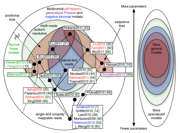
Figure 1. Models for RNA-Seq. The figure shows a Venn diagram (and the partially ordered set it induces) representing relationships among models. More general models are nested inside simpler models. Models in the same box are mathematically equivalent and the boxes are organized so that more complex models (i.e., with more parameters) are positioned above simpler models with fewer parameters. Model types are color coded and the dashed line separates multinomial, Poisson and generalized Poisson models and negative binomial models from normal linear models. This is because the MLE obtained using the normal linear models in the multi-read case approximates the MLE obtained using the Poisson or multinomial models. Two models [6, 49] are connected with dashed lines to [16] because they include normalization steps that are related to sequence bias correction, but they are not strictly special cases of [16]. Some models, such as [31, 59], include terms for modeling errors in mapping that in principle can be adapted to model any biases/features (meaning that the models are in some sense the most general possible) but if applied in that way would be impractical (see Remark 7) which is why they are not at the top of the hierarchy.

Remark 2 (Mathematical equivalence of models).

Figure 1 is more than just a cartoon organizing the models. Models from papers that appear in the same box are mathematically identical in terms of the quantification results they will produce (although not necessarily when used for differential analysis, see Section 7). We expand on this remark in the following sections. However, it is is important to note that although models may be equivalent, programs implementing them may not be. Implementation details are important and non-trivial and can result in programs with drastically different performance results and usability. For example, careful attention to data types and processing of reads in a manner tailored to the RNA-Seq protocol and sequencing technology used can improve quantification results.

3. Count based models

In this section we consider models that assume that all reads are single-end and that they map uniquely to transcripts. Such models are also known as “count based models”. In the simplest (generative) version of such a model, the transcriptome consists of a set of transcripts with different abundances, and a read is produced by choosing a site in a transcript for the beginning of the read uniformly at random from among all of the positions in the transcriptome.

Formally, if $T$ is the set of transcripts (with lengths $l_{t},t\in T$) we define $\rho=\{\rho_{t}\}_{t\in T}$ to be the relative abundances of the transcripts, so that $\sum_{t\in T}\rho_{t}=1$. We denote by $F$ the set of (single-end) reads and let $F_{t}\subseteq F$ be the set of reads mapping to transcript $t$. Furthermore, we use assume that all the reads in $F$ have the same length $m$. Note that in transcript $t$, the number of positions in which a read can start is $\tilde{l}_{t}=l_{t}-m+1$. The adjusted length $\tilde{l}_{t}$ is called the effective length of $t$.

In the generative model, first a transcript is chosen from which to select a read $f$ by

(1) $$\mathbb{P}(f\in t)\quad=\quad\frac{\rho_{t}\tilde{l}_{t}}{\sum_{r\in T}\rho_{r}\tilde{l}_{r}}.$$

Next, a position in that transcript is selected uniformly at random from among the $l_{t}-m+1$ positions. Thus, the likelihood of observing the reads $F$ as a function of the parameters $\rho$ is

(2) $$\mathcal{L}(\rho)\quad=\quad\prod_{t\in T}\prod_{f\in F_{t}}\left(\frac{\rho_{t}\tilde{l}_{t}}{\sum_{r\in T}\rho_{r}\tilde{l}_{r}}\cdot\frac{1}{\tilde{l}_{t}}\right).$$

If we denote by $X_{t}$ the number of reads mapping to transcript $t$, i.e. $X_{t}=|F_{t}|$, then we can rewrite the likelihood function as

(3) $$\mathcal{L}(\rho)\quad=\quad\prod_{t\in T}\left(\frac{\rho_{t}\tilde{l}_{t}}{\sum_{r\in T}\rho_{r}\tilde{l}_{r}}\cdot\frac{1}{\tilde{l}_{t}}\right)^{X_{t}}.$$

There is a convenient change of variables that reveals Equation 3 to be that of a log-linear model. Let $\alpha=\{\alpha_{t}\}_{t\in T}$ denote the probabilities of selecting a read from the different transcripts:

(4) $$\alpha_{t}\quad:=\quad\mathbb{P}(f\in t)\quad=\quad\frac{\rho_{t}\tilde{l}_{t}}{\sum_{r\in T}\rho_{r}\tilde{l}_{r}}.$$

Note that

(5) $$\sum_{t\in T}\alpha_{t}=1\mbox{ and }\alpha_{t}\geq 0\mbox{ for all }t.$$

Moreover, by Lemma 14 in the Supplementary Material of [61], for any probability distribution $\{\alpha_{t}\}_{t\in T}$ (i.e., satisfying the conditions of Equation 5), we can find a probability distribution $\rho$ so that Equation 4 is satisfied by setting

(6) $$\rho_{t}\quad=\quad\frac{\frac{\alpha_{t}}{\tilde{l}_{t}}}{\sum_{r\in T}\frac{\alpha_{r}}{\tilde{l}_{r}}}.$$

It follows that if Equation 3 is rewritten as

(7) $$\mathcal{L}(\alpha) = \prod_{t\in T}\left(\frac{\alpha_{t}}{\tilde{l}_{t}}\right)^{X_{t}}$$

(8) $$\propto \prod_{t\in T}\alpha_{t}^{X_{t}},$$

then the unique maximum likelihood solution for $\alpha$ can be transformed to the (unique) maximum likelihood solution for $\rho$. That is, from

(9) $$\hat{\alpha}_{t}\quad=\quad\frac{X_{t}}{N}$$

where $N=\sum_{t\in T}X_{t}$ is the total number of mapped reads, we can apply (6) to obtain that

(10) $$\hat{\rho}_{t} = \frac{\frac{\hat{\alpha}_{t}}{\tilde{l}_{t}}}{\sum_{r\in T}\frac{\hat{\alpha}_{r}}{\tilde{l}_{r}}}$$

(11) $$= \frac{X_{t}}{N}\cdot\frac{1}{\tilde{l}_{t}}\cdot\left(\frac{1}{\sum_{r\in T}\frac{X_{r}}{N\tilde{l}_{r}}}\right)$$

(12) $$\propto \frac{X_{t}}{\left(\frac{\tilde{l}_{t}}{10^{3}}\right)\cdot\left(\frac{N}{10^{6}}\right)}\cdot\left(\frac{1}{\sum_{r\in T}\frac{X_{r}}{N\tilde{l}_{r}}}\right)$$

(13) $$\propto \frac{X_{t}}{\left(\frac{\tilde{l}_{t}}{10^{3}}\right)\cdot\left(\frac{N}{10^{6}}\right)}.$$

Equation 13 is the RPKM (reads per kilobase per millions of reads mapped) formula with which to measure abundance from [41] (with the exception that in [41] $l_{t}$ is used instead of $\tilde{l}_{t}$). Note that RPKM can be viewed as a method because the term abbreviates the procedure of evaluating Equation 13. However the derivation above shows that RPKM is better thought of as a unit with which to measure relative transcript abundance because it is (up to a scalar factor) the maximum likelihood estimate for the $\rho$. Moreover, the statistical derivation of relative abundance in RPKM units reveals that effective length should be used instead of length, and it is evident that abundance estimates reported in RPKM units are not absolute, but rather relative.

Remark 3 (Normalizing the total number of reads).

The number $N$ used has been defined to be the number of mapped reads however we note that one can replace it by the number of sequenced reads if an extra faux “noise” transcript is included in the analysis as the source of the unmappable reads [31]. We use the term “noise” because unmappable reads may represent sequencing mistakes that result in meaningless data. Also, additional normalization steps may be applied to improve the robustness of relative transcript abundance estimates because extensive transcription of even a single gene can drastically affect RPKM values. To address this, quantile normalization was proposed in [7] and is implemented in a number of software packages for RNA-Seq analysis, e.g.[1, 26, 61].

The model described above is suitable for single isoform genes and is therefore appropriate in organisms such as bacteria where there is no splicing. However in higher Eukaryotes with extensive alternative splicing, alternative promoters, and possibly multiple polyadenylation sites, there may be ambiguity in the assignment of reads to transcripts and more complex models are necessary. Nevertheless, Equation 3 has been used for inference where reads map to multiple isoforms of a gene by using one of two different approaches that we refer to as projective normalization and restriction to uniquely mappable reads.

Projective normalization is an approach to estimating the relative abundance of genes consisting of multiple transcripts (corresponding to different isoforms) directly from the total number of reads mapping to the gene locus. The approach is based on Equation 13 but with $X_{t}$ replaced by the total number of reads mapping to the gene, and $l_{t}$ replaced by the total length of all the transcripts comprising the gene after projection into genomic coordinates (i.e., the union of all transcribed bases as represented in genomic coordinates). This approach has been used in a number of methods, including [14, 21, 49]. In [61, Proposition 3, Supplementary Material] it is proved that projective normalization always underestimates relative gene abundances, and in [66] empirical evidence is provided demonstrating that estimation of individual relative transcript abundances (by maximum likelihood) improves the accuracy of relative transcript abundance estimates. That is, the type of model presented in the next section improves on projective normalization.

Restriction to uniquely mappable reads consists of only utilizing reads that map uniquely to features of interest. Such an approach can be used for abundance estimation in multiple isoform genes by identifying unique features of transcripts (e.g. splice junctions unique to an isoform) and applying Equation 13 where $X_{t}$ is replaced by the read counts for that feature and $l_{t}$ is suitably adjusted for the length of the feature. Restriction to uniquely mappable reads has the major problem that valuable data may be omitted from analysis because it cannot be mapped to a unique transcript feature. For example, in many transcripts, the unique feature may consist of a single junction. The approach of [28] consists of the restriction to uniquely mappable reads via an adjustment of the length $l_{t}$ in Equation 13 whereas in [39] the correction is performed through adjustments to coverage.

Remark 4 (Species abundance estimation in metagenomics is related to transcriptome analysis).

The single end read model discussed above is relevant to abundance estimation in metagenomics, where the problem of estimating relative abundances of genomes in a community is related to relative transcript abundance estimation of single isoform genes. For example, a formula equivalent to Equation 13 appears in [2]. Another closely related problem is that of inferring haplotype frequencies from pooled samples [34]. These analogies between metagenomics, haplotype inference and transcriptomics can be extended further. For example, de novo transcriptome assembly requires the assembly of related sequences as in metagenome assembly. One key difference between metagenome and transcriptome assembly is that sequences from related species are more divergent than sequences of isoforms from a single gene.

4. Models for multi-reads: estimating isoform abundances

As discussed in the previous section, RNA-Seq allows for the estimation of the relative abundance of transcripts, however, this requires an extension of Equation 3 to allow for ambiguously mapped reads. In this section we show that the model of [69] is equivalent (with the exception of a length factor) to the model of [20], and show that the basis of the equivalence applies to many other models.

We begin by considering the likelihood function in [69] because that paper is, to our knowledge, the first publication of the inference model needed for transcript level relative abundance estimation from RNA-Seq. In [69] inference of relative abundances using expressed sequence tags (ESTs) is discussed, but in terms of the model there is no difference between ESTs and RNA-Seq with the exception of assumptions about whether EST counts scale with the length of transcripts, an issue we comment on below. The likelihood function that is derived describes the probability of obtaining $N$ reads from a transcriptome with $K$ transcripts. Using the notation of [69], we let ${\bf Y}=\{y_{i,k}\}_{i=1,k=1}^{N,K}$ be the matrix defined by $y_{i,k}=1$ if read $i$ aligns to transcript $k$ and $0$ otherwise. This matrix is called the compatibility matrix (for an example see Equation 38). The likelihood is then shown to be

(14) $$\mathcal{L}(\alpha)\quad=\quad\prod_{i=1}^{N}\left(\sum_{k=1}^{K}y_{i,k}\frac{\alpha_{k}}{\tilde{l}_{k}}\right).$$

Here $\alpha=(\alpha_{1},\ldots,\alpha_{K})$ is defined as in the previous section (in [69] $\alpha_{k}$ is denoted by $p_{k}$) and $k\in\{1,\ldots,K\}$ indexes the transcripts of the gene. We note that the denominator $\tilde{l}_{k}$ (length of isoform $k$) is missing in [69], which can be interpreted as an assumption that the frequency of ESTs from a transcript is directly proportional to its abundance (independent of the length of the transcript). This assumption makes sense based on the oligo(DT) priming strategy for ESTs, however some papers have suggested that truncated cDNAs contribute substantially to ESTs due to internal priming [42]. If this is the case then the addition of the length in the denominator is warranted; in the next section we derive a more general model of which Equation 14 is a special case, and in that derivation the reason for the denominator will become apparent.

Remark 5 (Length normalization).

The (deliberate) omission or missed inclusion of the denominator $\tilde{l}_{k}$ in [69] probably did not matter much in practice because the denominator is not needed if the lengths of all isoforms are equal. In that case, the likelihood function is changed by a scalar factor and therefore the maximum likelihood estimates for the incorrect and correct models will be the same. Since abundance estimates were only evaluated qualitatively in [69], the presence or absence of the denominator may not have changed results much. On the other hand, the paper [46] is specifically about RNA-Seq and therefore the omission of the denominator is an error.

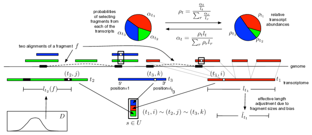
Figure 2. Notation used in describing RNA-Seq models. In this example there are three transcripts ($t_{1},t_{2},t_{3}$) whose abundances are denoted by $\rho_{t_{1}},\rho_{t_{2}},\rho_{t_{3}}$. Fragment lengths are distributed according to $D$, and the length of a transcript $t$ is denoted by $l_{t}$. The effective length $\tilde{l}_{t}$ is an adjustment of the length taking into account bias and fragment length constraints. Note that $l_{t_{2}}(f)$ is the length of the alignment of fragment $f$ to transcript $t_{2}$, and may be different from $l_{t_{1}}(f)$. In the example, transcripts $t_{2}$ and $t_{3}$ overlap in genomic coordinates. Three positions $(t_{1},i),(t_{2},j),(t_{3},k)$ have been selected, one from each transcript, that lie in the same equivalence class (i.e. cannot be distinguished in mapping). This is indicated by $(t_{1},i)\sim(t_{2},j)\sim(t_{3},k)$. Note that $(t_{2},j)\sim(t_{3},k)$ because they overlap in genomic coordinates whereas in the case of $(t_{1},i)$ the transcript is part of a different gene. A fragment $f$ is shown mapping to transcript $t_{2}$.

To describe the model of [20], we first introduce notation needed for multi-reads, which are reads that may map to multiple transcripts. Note that there are two reasons why reads may map to multiple transcripts: first, parts of transcripts may overlap in genomic coordinates (in the case of multi-isoform genes) and secondly, gene families may result in duplicated segments throughout the genome that lead to ambiguous read mappings (see Figure 2). In this section we restrict ourselves to the ambiguous mappings resulting from multiple isoforms of a single gene (to be consistent with the likelihood formulation of [69]), but we introduce notation for the general case as it will be useful later.

Let $\mathcal{T}=\{(t,i):t\in T,i\in\{1,\ldots,l_{t}\}\}$ be the set of all transcript positions. We first define a symmetric relation on the set of positions by the relation $(t,i)R(u,j)$ if there exists some fragment $f\in F$ so that the $3^{\prime}$ end of $f$ aligns to both $(t,i)$ and $(u,j)$. Note that if we allow for some mismatches in alignments, the relation $R$ may not be an equivalence relation. We will require the properties of equivalence relations in specifying models so we replace $R$ by its equivalence closure (also called the transitive closure) and denote the resulting equivalence relation by $\sim$.

The set of all equivalence classes is the quotient of $\mathcal{T}$ by $\sim$ and we denote it by $U=\mathcal{T}/\mathord{\sim}$. Given an equivalence class $s\in U$, $F_{s}\subseteq F$ is the set of all fragments aligning to some element in $s$ (note that this induces an equivalence relation on fragments). For simplicity, we also assume that every fragment with a $3^{\prime}$ alignment to some transcript $t$ has only one alignment of its $5^{\prime}$ end to a location in $t$.

In [20], it is assumed that for a set of aligned fragments $F$, for every $s\in U$ the number of reads starting at $s$ is Poisson distributed with rate parameter

(15) $$\lambda_{s}\quad=\quad\sum_{k=1}^{K}c_{s,k}\frac{\kappa_{k}}{\tilde{l}_{k}},$$

where $\kappa_{k}$ is a rate parameter for transcript $k$. Here ${\bf C}=\{c_{s,k}\}_{k=1,s\in U}^{K}$ is a site-transcript compatibility matrix with $c_{s,k}=1$ if transcript $k$ appears in some element of $s$, and $0$ otherwise. The parameters $\kappa_{k}$ are the expected number of reads from each transcript $k$. If the observed number of reads starting at $s$ is $X_{s}$, then the likelihood (Equation 2 in [20]) is given by

(16) $$\mathcal{L}(\kappa)\quad=\quad\prod_{s\in U}\left(\frac{e^{-\lambda_{s}}\lambda_{s}^{X_{s}}}{X_{s}!}\right).$$

At first glance Equations 14 and 16 look very different. The underlying models are distinct not just in name but in the generative model for RNA-Seq that they imply. In the Poisson model counts are Poisson distributed, which is only approximately the same as the count distribution from the multinomial model. It is therefore no surprise that the likelihood functions for the two different models have a different form. Moreover, neither the parameters $\alpha$ nor $\rho$ appear in Equation 16. However, we will see that Equation 16 can be written in terms of parameters equivalent to the $\alpha$ and that the two likelihood functions are maximized at the same value. This follows from an elementary and well-known equivalence between multinomial and Poisson log-linear models [25]. It is discussed in the RNA-Seq case in [51] but for completeness and clarity, we review the connection between the models in detail below.

Proposition 1.

Maximum likelihood parameters obtained via Equations 14 and 16 lead to exactly the same relative transcript abundance estimates.

Proof: Note that $\sum_{s\in U}X_{s}\mbox{ (from \cite[cite]{[\@@bibref{}{Jiang2009}{}{}]}) }=N\mbox{ (from \cite[cite]{[\@@bibref{}{Xing2006}{}{}]})}$ by definition. We will also define parameters $\beta_{k}:=\frac{\kappa_{k}}{N}$, $Z=\sum_{k=1}^{K}\beta_{k}$ and $\gamma_{k}=\frac{\beta_{k}}{Z}$. Note that $\sum_{k=1}^{K}\gamma_{k}=1$ and $\gamma_{k}\geq 0$, however since the $\kappa_{k}$ and $\beta_{k}$ are unconstrained the factor $Z$ can, a priori be arbitrary. The proof is based on the result that the maximum likelihood values for $\kappa$ are obtained when $Z=1$. We derive this after proving a simple combinatorial lemma that is useful inside the main argument. The lemma states that each $\kappa_{k}$ is counted once when summing over the equivalence classes of positions (and suitably normalizing by length):

Lemma 1.

$$\sum_{k=1}^{K}\kappa_{k}=\sum_{s\in U}\sum_{k=1}^{K}c_{s,k}\frac{\kappa_{k}}{\tilde{l}_{k}}.$$

Proof:

(17) $${\sum_{s\in U}\sum_{k=1}^{K}c_{s,k}\frac{\kappa_{k}}{\tilde{l}_{k}}} = \sum_{k=1}^{K}\sum_{s\in U}c_{s,k}\frac{\kappa_{k}}{\tilde{l}_{k}}$$

(18) $$= {\sum_{k=1}^{K}\tilde{l}_{k}\cdot\frac{\kappa_{k}}{\tilde{l}_{k}}}$$

(19) $$= \sum_{k=1}^{K}\kappa_{k}.\qed$$

From this it follows that

(20) $$\sum_{s\in U}\sum_{k=1}^{K}c_{s,k}\frac{\kappa_{k}}{\tilde{l}_{k}}=N\sum_{k=1}^{K}\beta_{k}$$

which is used in the proof of the proposition:

(21) $$\mathcal{L}(\kappa) = \prod_{s\in U}\left(\frac{e^{-\lambda_{s}}\lambda_{s}^{X_{s}}}{X_{s}!}\right)$$

(22) $$= e^{-\sum_{s\in s}\lambda_{s}}\prod_{s\in U}\left(\frac{\lambda_{s}^{X_{s}}}{X_{s}!}\right)$$

(23) $$\propto e^{-\sum_{s\in U}\sum_{k=1}^{K}c_{s,k}\frac{\kappa_{k}}{\tilde{l}_{k}}}\prod_{s\in U}\left(\sum_{k=1}^{K}c_{s,k}\frac{\kappa_{k}}{\tilde{l}_{k}}\right)^{X_{s}}$$

(24) $$= e^{-N\sum_{k=1}^{K}\beta_{k}}\prod_{s\in U}\left(\sum_{k=1}^{K}c_{s,k}N\frac{\beta_{k}}{\tilde{l}_{k}}\right)^{X_{s}}$$

(25) $$\propto \left(\frac{e^{-N\sum_{k=1}^{K}\beta_{k}}N^{N}}{N!}\right)\prod_{i=1}^{N}\left(\sum_{k=1}^{K}y_{i,k}\frac{\beta_{k}}{\tilde{l}_{k}}\right)$$

(26) $$\propto \left(\frac{e^{-NZ}(NZ)^{N}}{N!}\right)\prod_{i=1}^{N}\left(\sum_{k=1}^{K}y_{i,k}\frac{\gamma_{k}}{\tilde{l}_{k}}\right).$$

A key observation is that the parameter $Z$ in the left parentheses can be maximized independently of the $\gamma_{k}$ in the right parentheses. This is because $Z$ is unconstrained and the constraints on $\gamma$ do not involve $Z$ (the $\gamma$ only need to be non-negative and must sum to 1). The maximum likelihood estimate for the normalization constant $Z$ is $\hat{Z}=1$ and therefore $\hat{\beta}_{k}=\hat{\gamma}_{k}$ and the maximization of Equation 16 is equivalent to maximizing

(27) $$\mathcal{L}(\beta)\quad=\quad\prod_{i=1}^{N}\left(\sum_{k=1}^{K}y_{i,k}\frac{\beta_{k}}{\tilde{l}_{k}}\right)$$

where $\sum_{k=1}^{K}\beta_{k}=1$ and $\beta_{k}\geq 0$. The interpretation of the $\beta$ parameters in the Poisson model [20] is equivalent to the interpretation of the $\alpha$ parameters in [69], i.e. they are the probabilities for choosing reads from transcripts. Therefore, both model formulations are equivalent. ∎

5. A general model for RNA-Seq

In this section we present a general model for RNA-Seq that includes as special cases the other models discussed in this review. As before, we assume that every fragment with a $3^{\prime}$ alignment to some transcript $t$, has only one alignment of its $5^{\prime}$ end to a location in $t$. This means that the notion of the length of a fragment relative to a transcript is well-defined, and we denote this length by $l_{t}(f)$. This assumption is slightly restrictive, but simplifies a lot of the notation.

In a generative description of the model the $3^{\prime}$ end of a fragment is selected first. The probability of selecting the $3^{\prime}$ end from a specific site within a transcript depends on the abundance of the site relative to others (as determined by the relative abundance parameters $\rho$), on the local sequence content, and also on the relative position of the site within the transcript. Then a length for the fragment is selected according to a distribution $D$ and again according to the local sequence content.

We are interested in estimating the $\rho_{t}$, but due to the other parameters specifying a sequencing experiment we infer them indirectly. To specify the probability of a fragment with specific $5^{\prime}$ and $3^{\prime}$ ends, we require the following parameters:

• The fragment length distribution denoted $D$ which is a distribution whose support is the positive integers.

• Site specific bias: parameters $u_{(t,i)}$ denoting the $3^{\prime}$ site specific bias for position $i$ in transcript $t$. These parameter are non-negative real numbers (or “weights”), so that no bias corresponds to all $u_{(t,i)}=1$. Similarly, the $5^{\prime}$ site specific bias for position $i$ in transcript $t$ is denoted by $v_{(t,i)}$.

• Positional bias: parameters $w_{x}$ where $x\in[0,1]$ that are non-negative real numbers.

• Errors in reads: parameters $e_{t,f}$ denote the probability of observing the sequence in $f$ assuming that it was produced from transcript $t$. We assume (for simplicity) that every fragment could have been generated from at most one position in each transcript. The error probabilities $e_{t,f}$ can be estimated according to an error model for sequencing and based on the number and locations of mismatches/indels between $f$ and $t$. Note that $e_{t,f}$ can be viewed as a generalization of $y_{i,k}$ from the previous section where $i$ is replaced by $f$ and $k$ by $t$ and the values form a probability distribution rather than being restricted to the set $\{0,1\}$.

Our model specifies that the probability of selecting a fragment $f$ with $3^{\prime}$ end $(t,i)$ given that $f$ originates from transcript $t$ is

(28) $$\mathbb{P}(f^{3^{\prime}}=(t,i)|f\in t)\quad=\quad\frac{w_{\frac{i}{l_{t}}}\cdot u_{(t,i)}\cdot\sum_{j=1}^{i-1}\frac{D(i-j)}{\sum_{k=1}^{i-1}D(i-k)}v_{(t,j)}}{\tilde{l}_{t}},$$

where

(29) $$\tilde{l}_{t}\quad=\quad\sum_{i\in t}\left(w_{\frac{i}{l_{t}}}\cdot u_{(t,i)}\cdot\sum_{j=1}^{i-1}\frac{D(i-j)}{\sum_{k=1}^{i-1}D(i-k)}v_{(t,j)}\right).$$

As in Section 3, $\tilde{l}_{t}$ is the effective length of transcript $t$. The probability of selecting a fragment $f$ with $3^{\prime}$ end $(t,i)$ is now given by

(30) $$\mu_{(t,i)}:=\mathbb{P}(f^{3^{\prime}}=(t,i)) = \mathbb{P}(f\in t)\mathbb{P}(f^{3^{\prime}}=(t,i)|f\in t)$$

(31) $$= \alpha_{t}\frac{w_{\frac{i}{l_{t}}}\cdot u_{(t,i)}\cdot\sum_{j=1}^{i-1}\frac{D(i-j)}{\sum_{k=1}^{i-1}D(i-k)}v_{(t,j)}}{\tilde{l}_{t}},$$

and the conditional probability that a fragment $f$ with $3^{\prime}$ end $(t,i)$ has length $l_{t}(f)$ is

(32) $$\zeta^{f}_{(t,i)}\quad:=\quad\mathbb{P}(l(f)=l_{t}(f)|f^{3^{\prime}}=(t,i))\quad=\quad\frac{D(l_{t}(f))v_{(t,i-l+1)}}{\sum_{j=1}^{i-1}D(i-j)v_{(t,j)}}.$$

Therefore, the probability of generating a fragment $f$ of length $l_{t}(f)$ with $3^{\prime}$ end $(t,i)$ is

(33) $$\mathbb{P}(f^{3^{\prime}}=(t,i),l(f)=l_{t}(f)) = \mu_{(t,i)}\zeta^{f}_{(t,i)}$$

(34) $$= \alpha_{t}\frac{u_{(t,i)}\cdot v_{(t,i-l+1)}\cdot w_{\frac{i}{l_{t}}}\frac{D(l_{t}(f))}{\sum_{k=1}^{i-1}D(i-k)}}{\tilde{l}_{t}}.$$

The generative model we have just described is summarized in Figure 3.

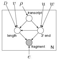
Figure 3. A generative (graphical) model for RNA-Seq.

We can now derive the likelihood for a set of fragments:

(35) $$\mathcal{L}(\alpha) = \prod_{s\in U}\prod_{f\in F_{s}}\sum_{(t,i)\in s}\alpha_{t}e_{t,f}\mathbb{P}(f^{3^{\prime}}=(t,i),l(f)=l_{t}(f)|f\in t)$$

(36) $$= \prod_{s\in U}\prod_{f\in F_{s}}\sum_{(t,i)\in s}\mu_{(t,i)}\zeta^{f}_{(t,i)}$$

(37) $$= \prod_{s\in U}\prod_{f\in F_{s}}\sum_{(t,i)\in s}\alpha_{t}e_{t,f}\frac{1}{\tilde{l}_{t}}\frac{D(l_{t}(f))}{\sum_{k=1}^{i-1}D(i-k)}u_{(t,i)}v_{(t,i-l_{t}(f)+1)}w_{\frac{i}{l_{t}}}.$$

This is a linear model (for fixed bias and error parameters) that is concave. In the next section we discuss how maximum likelihood estimates are obtained. Note that the inferred parameters $\hat{\alpha}$ can be translated to maximum likelihood estimates for the relative abundances $\hat{\rho}$ using Equation 6. Estimates are usually reported in units of FPKM (fragments per kilobase per million mapped fragments) [61] and are a scalar multiple of the $\hat{\rho}$ as in Equation 13.

In the case when bias is not modeled, i.e. $u_{(t,i)}=v_{(t,i)}=w_{(t,i)}=1$, then Equation 37 reduces to Equation 9 in the Supplementary Methods of [61] (with the slight difference in model as explained in Remark 6). This is also the model in [31] (with $\rho_{t}$ named $\theta_{t}$) and where the parameters $w_{(t,i)}$ are in the model but $u_{(t,i)}=v_{(t,i)}=1$. The paper [31] describes a single read model and the paired-end case will appear in [30]. This model is also the one used in [46] ($\alpha_{t}$ is named $P_{t}$, and formulated as an equivalent Poisson model).

Remark 6 (Directional assymetry in RNA-Seq).

There is some confusion in the current literature about how to model the generation of paired-end fragments in RNA-Seq experiments (e.g. in [12] three “strategies” are proposed). Some models consider a process where the $5^{\prime}$ end of a read is generated first (usually uniformly at random) followed by the $3^{\prime}$ end according to the fragment length distribution (normalized appropriately if the $5^{\prime}$ site is close to the $3^{\prime}$ end of the transcript). In the model described above, we have preferred to assume that the $3^{\prime}$ site is generated first, because that more closely mimics the actual protocol. Alternatively, one can assume that first a length is chosen according to the fragment length distribution, and then the $5^{\prime}$ and $3^{\prime}$ sites are chosen [52]. Such a model may better capture the fact that size selection follows reverse transcription and double stranded cDNA generation. It is at present unclear which formulation produces best estimates, but regardless of the choice the effect on the likelihood function is to slightly alter the form of the denominator.

Remark 7 (Errors in reads).

The error model we have included (parameters $e_{t,f}$) is analogous to the formulation in [59] and allows for a general and position-specific modeling of errors. However, it should be noted that there is a connection between errors and read mapping that can skew results even when errors are modeled. A read with a number of errors beyond the threshold of the mapping program used is not mapped, and this missing data problem is not addressed in our model. This issue can affect expression estimates, especially in the case of allele specific estimation [8] (see also remark below). It is therefore advisable to correct errors before mapping, using methods such as in [70]. In [59] all possible mapping are considered, i.e. the entire read-transcript compatibility matrix is constructed, and while this is the most general model for RNA-Seq since in principle the “error” model can capture any feature, it is impractical because the compatibility matrix is too large to work with explicitly in practical examples.

Remark 8 (Allele specific estimates).

It may be desirable to infer relative transcript abundances for individual haplotypes and this problem is addressed in various methods papers [6, 38, 46, 49, 62]. It is possible using the formalism we have described by simply doubling the number of transcripts (one for each haplotype) and utilizing the error parameters $e_{t,f}$ to obtain probabilities for each fragment originating from each of the haplotypes. Note that if the haplotypes are unknown then heterozygous sites can be inferred from the mapped fragments, but we do not consider that problem in this review as it is a mapping issue rather than a modeling problem.

The model we have presented is multinomial, however as discussed previously it can be formulated as an equivalent Poisson model. The details, and a proof that the two formulations are equivalent, is provided in Appendix I.

6. Inference

The single read single isoform model described in Section 2 is log-linear and therefore admits a closed form solution. Models that allow for ambiguous read mapping are no longer log-linear, but they do have nice properties and, assuming that bias effects are known, are concave [20, 61]. This means that numerical algorithms can be used to find the (unique) global maximum assuming that the model is identifiable.

Remark 9 (Identifiability).

Identifiability of RNA-Seq models is addressed in [24, 17] and appears even earlier in the computational biology literature in related models used in other applications (e.g.,[47]). Identifiability is the statistical property of “inference being possible”. Mathematically, that means that different parameter values (relative transcript abundances) generate different probability distributions on read counts. Testing for identifiability in our setting is equivalent to determining whether the compatibility matrix (Section 4) is full rank [17]. The identifiability problem is related to the transcript assembly problem, because with certain assumptions assemblies can be guaranteed to generate identifiable models for the aligned reads (this is the case with Cufflinks assemblies [61]).

Typically the Expectation-Maximization (EM) algorithm is used for optimization because of its simplicity in formulation and implementation.

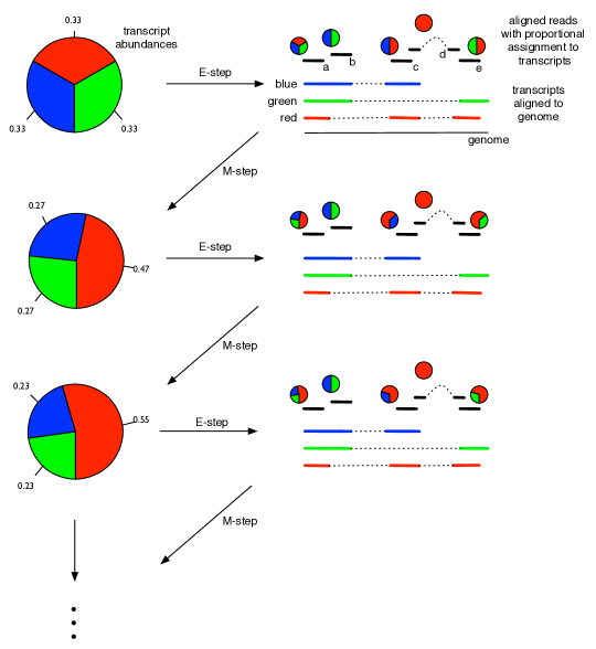
Figure 4. Illustration of the EM algorithm. The gene has three isoforms (red, green, blue) of the same length. There are five reads (a,b,c,d,e) mapping to the gene. One maps to all three isoforms, one only to red, and the other three to each of the three pairs of isoforms. Initially every isoform is assigned the same abundance ($\frac{1}{3},\frac{1}{3},\frac{1}{3}$). During the expectation (E) step reads are proportionately assigned to transcripts according to the isoform abundances. Next, during the maximization (M) step isoform abundances are recalculated from the proportionately assigned read counts. Thus, for example, the abundance of red after the first $M$ step is estimated by
$0.47=(0.33+0.5+1+0.5)/(2.33+1.33+1.33)$.

Example 1.

Consider a gene with three transcripts of equal length labeled red, green and blue, and with 5 single-end reads aligning to the transcripts according to the configuration shown in Figure 4. If the reads are labeled $a,b,c,d,e$ then the compatibility matrix (see Section 4) is

(38) $${\bf Y}\quad=\quad\bordermatrix{&a&b&c&d&e\cr{\tt red}&1&0&1&1&1\cr{\tt green}&1&1&0&0&1\cr{\tt blue}&1&1&1&0&0\cr}.$$

If the transcripts have abundances $\rho_{\mbox{\tt red}},\rho_{\mbox{\tt blue}},\rho_{\mbox{\tt green}}$ then the estimation of the $\rho$ (using the model in Section 3) is the mathematics problem of maximizing the likelihood function

(39) $$\mathcal{L}(\rho)\quad=\quad(\rho_{\mbox{\tt red}}+\rho_{\mbox{\tt blue}})(\rho_{\mbox{\tt red}}+\rho_{\mbox{\tt green}})(\rho_{\mbox{\tt blue}}+\rho_{\mbox{\tt green}})\rho_{\mbox{\tt red}}$$

subject to the constraint $\rho_{\mbox{\tt red}}+\rho_{\mbox{\tt blue}}+\rho_{\mbox{\tt green}}=1$. First, we note that the matrix $Y$ is full rank (rank=$3$) and therefore the model is identifiable.

Proposition 2.

The maximum likelihood solution is given by

(40) $$\hat{\rho}_{\mbox{\tt blue}}\quad=\quad\hat{\rho}_{\mbox{\tt green}}\quad=\quad\frac{7}{16}-\frac{\sqrt{17}}{16}\quad\approx\quad 0.18.$$

Proof: For notational simplicity we let $x=\rho_{\mbox{\tt blue}},y=\rho_{\mbox{\tt green}},z=\rho_{\mbox{\tt red}}$. The goal is to maximize $f(x,y,z)=z(1-x)(1-y)(1-z)$ subject to the constraint that $x+y+z=1$ and $x,y,z\geq 0$. Note that $f(x,y,z)=(x+y)(1-(x+y))(1+xy-(x+y))$. For any value $x+y$ at which $f$ is maximized, it follows that $xy$ must be maximized conditional on the sum, and that occurs at $x=y$. Therefore, the problem is equivalent to maximizing $2x(1-2x)(1+x^{2}-2x)$ where $0\leq x\leq\frac{1}{2}$. The maximum is at $\hat{x}=\frac{7}{16}-\frac{\sqrt{17}}{16}$.∎

In the EM algorithm, relative transcript abundances are first initialized (e.g. to the uniform distribution). In the expectation step every read (or fragment in the case of paired-end sequencing) is proportionately assigned to the transcripts it is compatible with, according to the relative transcript abundances. Then, in the maximization step, relative abundances are recalculated using the (proportionately) assigned fragment counts. In other words, the maximization step is the application of Equation 13 where counts are replaced by expected counts. A key property of the EM algorithm is that the likelihood increases at every step [45]. The illustration in Figure 4 shows 2 iterations of the algorithm and one can observe the convergence of $\rho$ with $\rho_{\mbox{\tt blue}}=0.33,0.27,0.23,\ldots$. EM theory states that $\rho_{\mbox{\tt blue}}$ will converge to the value in (40).

A derivation of the EM algorithm in the case of the model just described (from the general EM algorithm) is detailed in [69].

Remark 10 (Rescue for multi-reads).

The “rescue” method for multi-reads [41] is equivalent to one step of the EM algorithm (this important observation was made in [31]).

In some cases least squares has been used instead of the EM algorithm, e.g. in [5, 12, 18]. Least squares estimates are equivalent to maximum likelihood estimates under the assumption that the counts are normally distributed (with equal variances in [5], Poisson derived variances in [12] and possibly with a more complicated variance-covariance structure in [18] requiring an additional estimation procedure). Multivariate normal models approximate multinomial models well when counts are high but are not suitable when counts are low. There can be a computational problem with least squares inference. For example, the problem formulation in [18] results in an algorithm requiring matrix inversions of sizes exponential in the number of transcripts. Furthermore, the least squares approach requires constrained optimization (quadratic programming) because relative transcript abundances must be non-negative. This is done in [5, 12] but not in [18] where instead a heuristic is used and negative estimated values are truncated to zero.

The method in [38] is similar to the least squares approaches described above, except that $L_{1}$ minimization is performed. Unfortunately, the details of the method are not sufficiently well explained to permit a direct comparison to other published methods and therefore it has been omitted from Figure 1.

The inference approaches of [20, 22, 61] differ from other published methods in that they are Bayesian rather than frequentist. In [22], instead of using maximum likelihood to infer $\hat{\rho}$, the posterior distribution is computed assuming a Dirichlet prior. The approach of [20] and [61] is to use a Gaussian prior which is chosen according to the MLE estimated using the EM algorithm (with a variance-covariance matrix based on the inverse Fisher information matrix from asymptotic MLE theory). An importance sampling procedure is then used to sample from the posterior distribution [33].

7. Differential analysis

Accurate relative transcript abundance estimates are important not just for comparing isoform abundances to each other, but also for many other RNA-Seq applications. A common question for which RNA-Seq is now used is to determine differentially transcribed RNAs (the term differential expression is frequently used but it is a misnomer and the term differential analysis is more accurate). Clearly accurate relative transcript abundance estimates are desirable in order to have power to detect differentially transcribed RNAs.

First we note that the multinomial models and Poisson models are equivalent in terms of differential analysis by virtue of the following elementary lemma:

Lemma 2.

Suppose $X_{1},\ldots,X_{n}$ are Poisson distributed with rates $\lambda_{1},\ldots,\lambda_{n}$ respectively. Then the distribution of $X_{1},\ldots,X_{n}$ conditioned on the sum $\sum_{i=1}^{n}X_{i}=N$ is multinomial.

These models, however have been found to be unsatisfactory for differential analysis because observed counts in technical, and even more so, biological replicates, do not behave multinomially. This is a common phenomenon observed in count-based experiments, and is referred to as over- or under- dispersion. Papers such as [1, 53, 56, 65] have proposed numerous alternatives to the multinomial model, for example assuming instead that counts are distributed according to a negative binomial, or generalized Poisson distribution. The differences between the methods [1, 53, 65] are mainly in how they estimate parameters, and a thorough discussion of how they differ is beyond the scope of this review. A key point, however, is that these approaches all focus on single-end uniquely mappable reads (i.e., the models in Section 3) and this has the major drawback of not allowing for differential analysis of individual transcripts in multi isoform genes, and of biasing results in gene families. Recent versions of the Cufflinks software [61] address this problem.

Remark 11 (Models, quantification and differential analysis).

We can now summarize the relevance of model selection for quantification and differential analysis as follows: Multinomial models and Poisson models are equivalent for quantification and for differential analysis (by virtue of Lemma 2). Negative binomial models are equivalent to multinomial models for quantification, but result in different (more conservative) results in differential analysis. Negative binomial models will produce different relative abundance estimates if generalized to the multi-read case but this has not yet been done. Normal linear models in the multi-read case result in different quantification and differential analysis results although they can be viewed as an approximation of the Poisson (or multinomial) models.

Finally, we note that optimized differential analysis of RNA-Seq experiments involves not only the selection of appropriate models and robust parameters estimation techniques but also appropriate experimental design [3].

8. Discussion and future directions

Models of RNA-Seq have advanced greatly in complexity and accuracy in the three years since the protocol was developed; in this review alone we have discussed more than 30 different methods that have been published. At the same time, there has been considerable progress in RNA-Seq technology, both in protocol development to reduce bias [29], and in sequencing technology that has resulted in much higher throughput [36]. These developments have led to remarkable progress in the accuracy of RNA-Seq based relative transcript abundance estimates in the short time since introduction of the technology. Eventually, as single molecule based technologies mature [50] and reads as long as entire transcripts can be produced [10], RNA-Seq will be “solved” in the sense that a single sequencing experiment will directly reveal the transcriptome being queried.

However with present technologies, and for the foreseeable future, improvements in RNA-Seq modeling are required to best utilize the data produced in RNA sequencing experiments. Furthermore, related technologies such as ribosomal profiling [19] require similar models because they rely on probabilistically assigning short reads to transcripts, yet they are limited by experimental rather than technological issues and the types of models we have described are therefore likely to be relevant for a long time.

A key question, in light of the many remarks we have made, is what models are relevant in practice, and how a model should be selected in conjunction with available sequencing technology. We begin with what we believe is the most important consideration:

Remark 12 (Read length and model).

The multi-read models presented in Section 3 that are suitable for reads which may map to multiple transcripts are essential for accurate quantification and differential analysis, even in organisms without splicing or with few multi-isoform genes. This is because of multi-gene families, and repeated domains, that can result in ambiguously mapped reads. This issue is particularly pronounced for short reads ($<50$’bp) [62, Table 1]. Longer reads and fragments mitigate multi-mapping issues due to gene duplicates, however in that case effective length corrections (Section 2) become very important. Use of Equation 13 with $l_{t}$ in the denominator instead of $\tilde{l}_{t}$ can affect relative abundance estimates by up to 30% for fragments with an average size of 200 (as is common in current protocols). It is important to note that the improvement in mapping of longer reads may come at the expense of the number of reads, and in [31] it is shown that more short reads are better for accurate quantification than fewer long reads. However, it should also be noted that for other RNA-Seq analysis problems, e.g. transcriptome assembly, long reads and fragments are crucial [61].

The simplest models discussed in this review assume uniformity of fragment location across transcripts, yet observed data does not conform to this assumption (see, e.g. [11, Figure 6]). It is therefore highly desirable to model bias using more general models, and results in recent papers such as [52] show better agreement between RNA-Seq and qRT-PCR based estimates when bias is taken into account. Even newer protocols result in biases [29] that can be mitigated via appropriate modeling. However even with current state of the art corrections for sequence and positional bias, unexplained biases in the data continue to be observed [32, 52]. A possible source of bias that remains to be explored and may affect RNA-Seq experiments is secondary structure in RNA, and the effect it may have on the various fragmentation and reverse transcription steps of existing protocols. Recent progress on sequencing based assays for measuring structural features of RNA molecules may help to establish a connection between structure and bias, and to quantify the effect if it exists [4, 23, 35, 63].

A crucial area where progress is needed is in the assessment of accuracy of RNA-Seq. The exact accuracy of relative abundance estimates based on the techniques reviewed in this paper is currently unknown, and benchmarks with respect to qRT-PCR [7] or nanostring [52] have cast doubt on whether those technologies are more accurate than RNA-Seq and suitable as “gold standards”. Most importantly, there is a need for systematic benchmarks where abundances are known a priori, yet where experiments mimic the complexities of in vivo transcriptomes.

Another aspect of RNA-Seq that has yet to be fully explored is the connection between relative abundance estimation and transcriptome assembly. In [61], it is shown that an incomplete transcriptome can bias relative abundance estimates. For this reason, it was proposed that analyses should be performed with respect to an assembly generated from the data, rather than using a “reference” annotation. Indeed, in almost every RNA-Seq study performed to date many novel transcripts have been detected, even in extensively annotated species such as Drosophila [13]. Transcriptome assembly is therefore crucial at the present time for accurate relative abundance estimation.

Accurate and complete transcriptome assembly is, in turn, dependent on the ability to accurately quantify relative transcript abundances. This is because fragment lengths are currently much shorter than transcript lengths, and therefore local estimates of relative abundance are the only information available for phasing distant exons during assembly [64]. For this reason, statistical assembly approaches such as [27] need to be developed for transcriptome assembly. Despite initial work by a number of groups (personal communication), the problem of how to perform statistical assembly efficiently and accurately remains open.

9. Acknowledgments

I thank Adam Roberts and Cole Trapnell for many helpful discussions that clarified our understanding of RNA-Seq and that led to many of the remarks in this paper. Meromit Singer, during the course of many discussions with me, questioned the relevance and interpretation of alternative likelihood formulations for methyl-Seq models; those conversations led to similar questions about RNA-Seq models, and finally to the comments on the equivalence between multinomial and Poisson models for RNA-Seq discussed in Section 4 and Appendix I. Colin Dewey provided many helpful suggestions and comments after reviewing a preliminary version of the manuscript. Finally, thanks to Sharon Aviran, Nicolas Bray, Ingileif Hallgrímsdóttir, Valerie Hower, Aaron Kleinman, Megan Owen, Harold Pimentel, Atif Rahman, Adam Roberts, Meromit Singer and Cole Trapnell for valuable comments and insights during the writing of this paper.

Appendix I: Equivalence between the paired-end Poisson and multinomial models for RNA-Seq

In this section we show that the general model described in Section 5 is equivalent (in the sense discussed in Section 4) to a Poisson model for paired-end reads (with the same bias model).

To describe the Poisson model we need some extra notation: a weak composition of $n$ into $k$ parts is an ordered tuple of non-negative integers ${\bf c}=(c_{1},\ldots,c_{k})$ such that $c_{1}+\cdots+c_{k}=n$. If ${\bf c}$ is a weak composition of $n$ we write ${\bf c}\vdash n$. We note that the number of weak compositions of $n$ into $k$ parts is

(41) $${n+k-1\choose k-1}\quad=\quad{n+k-1\choose n}$$

For convenience, we use the notation $|{\bf c}|$ for the number of parts in a composition.

We will make use of multinomial coefficients, and we use the convention that

(42) $${n\choose{\bf c}}\quad=\quad{n\choose c_{1},\ldots,c_{k}}\quad=\quad\frac{n!}{c_{1}!c_{2}!\cdots c_{k}!}$$

where ${\bf c}\vdash n=(c_{1},\ldots,c_{k})$ is a composition of $n$ into $k$ parts.

Finally, we note that a function $P:F_{s}\rightarrow s$ induces a weak composition of $|F_{s}|$ where the composition is given by the cardinalities of the sets $\{f:P(f)=(t,i)\}$ as $(t,i)$ ranges over the elements of $s$. We use $|P|$ to denote this composition.

Example 2.

Suppose that $S=\{(t_{1},4),(t_{2},6),(t_{3},3)\}$ is an equivalence class with 3 elements corresponding to three distinct positions in three different transcripts ($t_{1},t_{2},t_{3}$). Suppose that the set of fragments whose $3^{\prime}$ ends align to $S$ consists of four fragments: $F_{s}=\{f_{1},f_{2},f_{3},f_{4}\}$. There are $3^{4}=81$ different functions $P:F_{s}\rightarrow S$. If $P(f_{1})=P(f_{3})=(t_{1},4)$ and $P(f_{2})=P(f_{4})=(t_{3},3)$ then $P$ induces the weak composition ${\bf c}\vdash 4$ with $3$ parts given by ${\bf c}=(2,0,2)$. We denote this weak composition ${\bf c}$ by $|P|$.

We conclude by highlighting an elementary, yet crucial step in the derivation of the likelihood function. Suppose that $\{a_{ij}\}_{i=1,j=1}^{n,m}$ are $n\cdot m$ indeterminates. Then the following two polynomials are equal:

(43) $$\sum_{f:[n]\rightarrow[m]}\prod_{i=1}^{n}a_{i,f(i)}\quad=\quad\prod_{i=1}^{n}\sum_{j=1}^{m}a_{ij}.$$

The expression on the left in (43) consists of $m^{n}$ monomials, each with $n$ terms, but the factored expression on the right shows that the polynomial can be evaluated using only $O(nm)$ operations.

Next we turn to the likelihood function. Let $s\in U=\mathcal{T}/\mathord{\sim}$ and let ${\bf c}\vdash|F_{s}|$ be a weak composition of $|F_{s}|$. We define $\eta_{s,{\bf c}}$ to be the sum

(44) $$\eta_{s,{\bf c}}\quad=\quad\sum_{P:F_{s}\rightarrow s:|P|={\bf c}}\prod_{f\in F_{s}}\zeta^{f}_{P(f)}e_{P(f),f}.$$

The number $\eta_{s,{\bf c}}$ is the probability of observing the assignment of fragments in $F_{s}$ to elements of $s$ where the numbers of fragments originating from each $(t,i)\in s$ is given by $c_{(t,i)}$.

Our model for RNA-Seq is Poisson, which means that we assume that the number of fragments ending at a given site is Poisson distributed. Specifically, we assume that the number of fragments with $3^{\prime}$ end $(t,i)$ is

(45) $$\lambda_{(t,i)}\quad=\quad\kappa_{t}\frac{w_{\frac{i}{l_{t}}}\cdot u_{(t,i)}\cdot\sum_{j=1}^{i-1}\frac{D(i-j)}{\sum_{k=1}^{i-1}D(i-k)}v_{(t,j)}}{\tilde{l}_{t}},$$

where the notation is the same as that in Section 5. As in Section 4, we let $\beta_{t}=\frac{\kappa_{t}}{N}$. The likelihood function we now derive directly generalizes that of [20] to paired-end reads. The likelihood function is now given by

(46) $$\mathcal{L} = \prod_{s\in U}\left(\sum_{{\bf c}\,\vdash|F_{s}|:|{\bf c}|=|s|}\frac{1}{{|F_{s}|\choose{\bf c}}}\left(\prod_{(t,i)\in s}\eta_{s,{\bf c}}e^{-\lambda_{(t,i)}}\frac{\lambda_{(t,i)}^{c_{(t,i)}}}{c_{(t,i)}!}\right)\right)$$

(47) $$= \prod_{s\in U}\frac{1}{|F_{s}|!}\left(\sum_{{\bf c}\,\vdash|F_{s}|:|{\bf c}|=|s|}\left(\prod_{(t,i)\in s}c_{(t,i)}!\eta_{s,{\bf c}}e^{-\lambda_{(t,i)}}\frac{\lambda_{(t,i)}^{c_{(t,i)}}}{c_{(t,i)}!}\right)\right)$$

(48) $$\propto \prod_{s\in U}\left(\prod_{(t,i)\in s}e^{-\lambda_{(t,i)}}\right)\left(\sum_{{\bf c}\,\vdash|F_{s}|:|{\bf c}|=|s|}\prod_{(t,i)\in s}\eta_{s,{\bf c}}\lambda_{(t,i)}^{c_{(t,i)}}\right)$$

(49) $$= \prod_{s\in U}e^{-\sum_{(t,i)\in s}\lambda_{(t,i)}}\left(\sum_{{\bf c}\,\vdash|F_{s}|:|{\bf c}|=|s|}\left(\sum_{P:F_{s}\rightarrow s:|P|={\bf c}}\prod_{f\in F_{s}}\zeta^{f}_{P(f)}e_{P(f),f}\lambda_{P(f)}\right)\right)$$

(50) $$= \prod_{s\in U}e^{-\sum_{(t,i)\in s}\lambda_{(t,i)}}\left(\sum_{P:F_{s}\rightarrow s}\prod_{f\in F_{s}}\zeta^{f}_{P(f)}\lambda_{P(f)}\right)$$

(51) $$= \prod_{s\in U}e^{-\sum_{(t,i)\in s}\lambda_{(t,i)}}\left(\prod_{f\in F_{s}}\sum_{(t,i)\in s}\zeta^{f}_{(t,i)}\lambda_{(t,i)}\right)$$

(53) $$= \left(\prod_{s\in U}e^{-N\sum_{(t,i)\in s}\beta_{t}\frac{w_{\frac{i}{l_{t}}}\cdot u_{(t,i)}\cdot\sum_{j=1}^{i-1}\frac{D(i-j)}{\sum_{k=1}^{i-1}D(i-k)}v_{(t,j)}}{\tilde{l}_{t}}}\right)$$

$$\times\left(\prod_{s\in U}\prod_{f\in F_{s}}\sum_{(t,i)\in s}\beta_{t}e_{t,f}\frac{u_{(t,i)}\cdot v_{(t,i-l+1)}\cdot w_{\frac{i}{l_{t}}}\frac{D(l)}{\sum_{k=1}^{i-1}D(i-k)}}{\tilde{l}_{t}}\right)$$

(54) $$= e^{-N\sum_{t\in T}\beta_{t}}\times\left(\prod_{s\in U}\prod_{f\in F_{s}}\sum_{(t,i)\in s}\beta_{t}e_{t,f}\frac{u_{(t,i)}\cdot v_{(t,i-l+1)}\cdot w_{\frac{i}{l_{t}}}\frac{D(l)}{\sum_{k=1}^{i-1}D(i-k)}}{\tilde{l}_{t}}\right).$$

We note that the term in parentheses in (54) is exactly the same expression as (37) with $\alpha_{t}$ replaced by $\beta_{t}$. As in the derivation in Section 3, it is easy to see that the likelihood functions are maximized at $\hat{\alpha}=\hat{\beta}$.

Appendix II: Notation

The notation table below shows the names of all the variables we use. It is divided into parts using four divisions: the first is notation for structures independent of an experiment (transcripts). The second is notation for data from the experiment (fragments and their alignments). The third is notation for the parameters of the model. The fourth consists of helper variables that are calculated from the primary variables in the first three categories.

$T$	set of transcripts
$\mathcal{T}$	set of transcripts together with their positions
$l_{t}$	length of transcript $t$
$F$	set of fragments
$F_{s}$	The set of fragments aligning to an equivalence class $s$ of alignment positions
$l_{t}(f)$	the length of a fragment alignment to a transcript $t$
$X_{t}$	number of fragments aligning to a transcript $t$
$X_{s}$	number of fragments ending (or starting) at a site in $s$
Y	compatibility matrix (between fragments and transcripts)
C	compatibility matrix (between sites and transcripts)
$\rho_{t}$	abundance of transcript $t$
$\lambda_{(t,i)}$	Poisson rate parameter for position $i$ in transcript $t$
$\alpha_{t}$	probability of selecting a fragment from transcript $t$ in the multinomial model
$\kappa_{t}$	Poisson rate parameter for transcript $t\in T$
$\beta_{t}$	The probability of selecting a fragment from transcript $t$ in the Poisson model
$e_{t,f}$	probability of observing $f$ given the sequence in $t$
$u_{(t,i)}$	$3^{\prime}$ bias weight
$v_{(t,i)}$	$5^{\prime}$ bias weight
$w_{x}$	positional weight where $x\in[0,1]$
$D$	Fragment length distribution
$\tilde{l}_{t}$	effective length of transcript $t$
$\eta_{S,{\bf c}}$	Probability that fragments were sequenced from position $i$ of transcript $t$
$\zeta^{f}_{(t,i)}$	Probability of selecting a fragment of length $l_{t}(f)$ given $3^{\prime}$ end $(t,i)$

Table 1. Notation.

References

- [1] S Anders and W Huber, Differential expression analysis for sequence count data, Genome Biology 11 (2010), R106.
- [2] FE Angly, D Willner, A Prieto-Davó, RA Edwards, R Schmieder, R Vega-Thurber, DA Antonopoulos, K Barott, MT Cottrell, et al., The GAAS metagenomic tool and its estimations of viral and microbial average genome size in four major biomes, PLoS Computational Biology 5 (2009), e1000593.
- [3] PL Auer and RW Doerge, Statistical design and analysis of RNA sequencing data, Genetics 185 (2010), 405–416.
- [4] S Aviran, C Trapnell, JB Lucks, SA Mortimer, S Luo, GP Schroth, JA Doudna, AP Arkin, and L Pachter, Modeling and automation of sequencing-based characterization of RNA structure, Proceedings of the National Academy of Sciences (2011), in press.
- [5] R Bohnert and G Rätsch, rQuant.web: a tool for RNA-Seq-based transcript quantitation, Nucleic Acids Research 38 (2010), W348–W351.
- [6] JH Bullard, Y Mostovoy, S Dudoit, and RB Brem, Polygenic and directional regulatory evolution across pathways in Saccharomyces, Proceedings of the National Academy of Sciences 107 (2010), 5058–5063.
- [7] JH Bullard, E Purdom, KD Hansen, and S Dudoit, Evaluation of statistical methods for normalization and differential expression in mRNA-Seq experiments, BMC Bioinformatics 11 (2010), 94.
- [8] JF Degner, JC Marioni, AA Pai, JK Pickrell, E Nkadori, Y Gilad, and JK Pritchard, Effect of read-mapping biases on detecting allele-specific expression from RNA-sequencing data, Bioinformatics 25 (2009), 3207–3212.
- [9] F Denoeud, J-M Aury, C Da Silva, B Noel, O Rogier, M Delledonne, M Morgante, G Valle, P Wincker, C Scarpelli, et al., Annotating genomes with massive-scale RNA sequencing, Genome Biology 9 (2008), R175.
- [10] J Eid, A Fehr, J Gray, K Luong, J Lyle, G Otto, P Peluso, D Rank, P Baybayana, B Bettman, et al., Real-time DNA sequencing from single polymerase molecules, Science 323 (2009), 133–138.
- [11] SN Evans, V Hower, and L Pachter, Coverage statistics for sequence census methods, BMC Bioinformatics 11 (2010), 430.
- [12] J Feng, W Li, and T Jiang, Inference of isoforms from short sequence reads, Research in Computational Molecular Biology (B Berger, ed.), vol. 6044, 2010, pp. 138–157.
- [13] BR Graveley, AN Brooks, JW Carlson, MO Duff, JM Landolin, L Yang, CG Artieri, MJ van Baren, N Boley, BW Booth, et al., The developmental transcriptome of Drosophila melanogaster, Nature 471 (2011), 473–479.
- [14] M Griffith, OL Griffith, J Mwenifumbo, R Goya, AS Morrissy, RD Morin, R Corbett, MJ Tang, Y-C Hou, TJ Pugh, et al., Alternative expression analysis by RNA sequencing, Nature Methods 7 (2010), 843–847.
- [15] BJ Haas and MC Zody, Advancing RNA-Seq analysis, Nature Biotechnology 28 (2010), 421–423.
- [16] KD Hansen, SE Brenner, and S Dudoit, Biases in Illumina transcriptome sequencing caused by random hexamer priming, Nucleic Acids Research 38 (2010), e131.
- [17] D Hiller, H Jiang, W Xu, and WH Wong, Identifiability of isoform deconvolution from junction arrays and RNA-Seq, Bioinformatics 25 (2009), 3056–3059.
- [18] BE Howard and S Heber, Towards reliable isoform quantification using RNA-Seq data, BMC Bioinformatics 11 (Suppl 3) (2010), S6.
- [19] N Ingolia, S Ghaemmahammi, JRS Newman, and JS Weissman, Genome wide analysis in vivo of translation with nucleotide resolution using ribosomal profiling, Science 324 (2009), 218–223.
- [20] H Jiang and WH Wong, Statistical inferences for isoform expression in RNA-Seq, Bioinformatics 25 (2009), 1026–1032.
- [21] M Kasowski, F Grubert, C Heffelfinger, M Hariharan, A Asabere, SM Waszak, L Habegger, J Rozowsky, M Shi, AE Urban, et al., Variation in Transcription Factor Binding Among Humans, Science 328 (2010), 232–235.
- [22] Y Katz, ET Wang, EM Airoldi, and CB Burge, Analysis and design of RNA sequencing experiments for identifying isoform regulation, Nature Methods 7 (2010), 1009–1015.
- [23] M Kertesz, Y Wan, E Mazor, JL Rinn, RC Nutter, HY Chang, and E Segal, Genome-wide measurement of RNA secondary structure in yeast, Nature 467 (2010), 103–107.
- [24] V Lacroix, M Sammeth, R Guigó, and A Bergeron, Exact transcriptome reconstruction from short sequence reads, WABI 2008, Lecture Notes in Bioinformatics (KA Crandall and J Lagergren, eds.), vol. 5251, 2008, pp. 50–63.
- [25] JB Lang, On the comparison of multinomial and Poisson log-linear models, Journal of the Royal Statistical Society B 58 (1996), 253–266.
- [26] B Langmead, KD Hansen, and JT Leek, Cloud-scale RNA-sequencing differential expression analysis with Myrna, Genome Biology 11 (2010), R83.
- [27] J Laserson, V Jojic, and D Koller, Genovo: de novo assembly for metagenomes, Journal of Computational Biology 18 (2011), 429–443.
- [28] S Lee, CH Seo, B Lim, JO Yang, J Oh, M Kim, S Lee, B Lee, C Kang, and S Lee, Accurate quantification of transcriptome from RNA-Seq data by effective length normalization, Nucleic Acids Research 39 (2010), e9.
- [29] J Levin, X Adiconis, M Yassour, D Thompson, M Guttman, M Berger, L Fan, N Friedman, C Nussbaum, A Gnirke, et al., Development and evaluation of RNA-seq methods, Genome Biology 11 (Suppl 1) (2010), P26.
- [30] B Li and C Dewey, RSEM: accurate quantification of gene and isoform expression from RNA-Seq data, submitted.
- [31] B Li, V Ruotti, RM Stewart, JA Thomson, and CN Dewey, RNA-Seq gene expression estimation with read mapping uncertainty, Bioinformatics 26 (2010), 493–500.
- [32] J Li, H Jiang, and WH Wong, Modeling non-uniformity in short-read rates in RNA-Seq data, Genome Biology 11 (2010), R50.
- [33] JS Liu, Monte Carlo Strategies in Scientific Computing, Springer, 2008.
- [34] Q Long, DC Jeffares, Q Zhang, K Ye, V Nizhynska, Z Ning, C Tyler-Smith, and M Nordborg, PoolHap: inferring haplotype frequencies from pooled samples by next generation sequencing, PLoS One 5 (2011), e15292.
- [35] JB Lucks, SA Mortimer, C Trapnell, S Luo, GP Schroth, L Pachter, JA Doudna, and AP Arkin, SHAPE-Seq: Multiplexed RNA secondary and tertiary structure determination, Proceedings of the National Academy of Sciences (2011), in press.
- [36] ER Mardis, A decade’s perspective on DNA sequencing technology, Nature 470 (2011), 198–203.
- [37] JC Marioni, CE Mason, SM Mane, M Stephens, and Y Gilad, RNA-seq: An assessment of technical reproducibility and comparison with gene expression arrays, Genome Research 18 (2008), 1509–1517.
- [38] SB Montgomery, M Sammeth, M Gutierrez-Arcelus, RP Lach, C Ingle, J Nisbett, R Guigo, and ET Dermitzakis, Transcriptome genetics using second generation sequencing in a Caucasian population, Nature 464 (2010), 773–777.
- [39] RD Morin, M Bainbridge, A Fejes, M Hirst, M Krzywinski, TJ Pugh, H McDonald, R Varhol, SJM Jones, and MA Marra, Profiling the HeLa S3 transcriptome using randomly primed cDNA and massively parallel short-read sequencing, BioTechniques 45 (2008), 81–94.
- [40] A Mortazavi, EM Schwartz, B Williams, L Schaeffer, I Antoshechkin, BJ Wold, and PW Sternberg, Scaffolding a Caenorhabditis nematode genome with RNA-seq, Genome Research 20 (2010), 1740–1747.
- [41] A Mortazavi, BA Williams, K McCue, L Schaeffer, and B Wold, Mapping and quantifying mammalian transcriptomes by RNA-Seq, Nature Methods 5 (2008), 585–587.
- [42] DK Nam, S Lee, G Zhou, X Cao, C Wang, T Clark, J Chen, JD Rowley, and SM Wang, Oligo(dT) primer generates a high frequency of truncated cDNAs through internal poly(A) priming during reverse transcription, Proceedings of the National Academy of Sciences 99 (2002), 6152–6156.
- [43] M Nicolae, S Mangul, I Măndoiu, and A Zelikovsky, Estimation of alternative splicing isoform frequencies from RNA-Seq data, Research in Computational Molecular Biology (V Moulton and M Singh, eds.), vol. 6293, 2010, pp. 202–214.
- [44] A Oshlack, MD Robinson, and MD Young, From RNA-Seq reads to differential expression results, Genome Biology 11 (2010), 220.
- [45] L Pachter and B Sturmfels (eds.), Algebraic Statistics for Computational Biology, Cambridge University Press, 2005.
- [46] B Paşaniuc, N Zaitlen, and E Halperin, Accurate Estimation of Expression Levels of Homologous Genes in RNA-seq Experiments, Research in Computational Molecular Biology (B Berger, ed.), vol. 6044/2010, 2010, pp. 397–409.
- [47] I Pe’er and JS Beckmann, Recovering frequencies of known haplotype blocks from single-nucleotide polymorphism allele frequencies, Genetics 166 (2004), 2001–2006.
- [48] S Pepke, B Wold, and A Mortazavi, Computation for ChIP-seq and RNA-seq studies, Nature Methods 6 (2009), S22–S32.
- [49] JK Pickrell, JC Marioni, AA Pai, JF Degner, BE Engelhardt, E Nkadori, J-B Veyrieras, M Stephens, Y Gilad, and JK Pritchard, Understanding mechanisms underlying human gene expression variation with RNA sequencing, Nature 464 (2010), 768–772.
- [50] T Raz, M Causey, DR Jones, A Kieu, S Letovsky, D Lipson, E Thayer, JF Thompson, and PM Milos, RNA Sequencing and Quantitation Using the Helicos Genetic Analysis System, High-Throughput Next Generation Sequencing: Methods in Molecular Biology, vol. 733, Springer, 2011, pp. 37–49.
- [51] H Richard, MH Schultz, M Sultan, A Nürnberger, S Schrinner, D Balzereit, E Dagand, A Rasche, H Lehrach, M Vingron, et al., Prediction of alternative isoforms from exon expression levels in RNA-Seq experiments, Nucleic Acids Research 38 (2010), e112.
- [52] A Roberts, C Trapnell, J Donaghey, JL Rinn, and L Pachter, Improving RNA-Seq expression estimates by correcting for fragment bias, Genome Biology 12 (2011), R22.
- [53] MD Robinson, DJ McCarthy, and GK Smyth, edgeR: a Bioconductor package for differential expression analysis of digital gene expression data, Bioinformatics 26 (2010), 139.
- [54] J Salzman, H Jiang, and WH Wong, Statistical modeling of RNA-Seq data, Statistical Science (2011), in press.
- [55] TM Smith, NE Olson, and D Smith, Making cancer transcriptome sequencing assays practical for the research and clinical scientist, Genome Biology 11 (Suppl 1) (2010), P39.
- [56] S Srivastava and L Chen, A two-parameter generalized Poisson model to improve the analysis of RNA-seq data, Nucleic Acids Research 38 (2010), e170.
- [57] M Sultan, MH Schultz, H Richard, A Magen, A Klingenhoff, M Scherf, M Seifert, T Borodina, A Soldatov, D Parkhomchuk, et al., A global view of gene activity and alternative splicing by deep sequencing of the human transcriptome, Science 321 (2008), 956–960.
- [58] F Tang, C Barbacioru, Y Wang, E Nordman, C Lee, N Xu, X Wang, J Bodeau, BB Tuch, A Siddiqui, et al., mRNA-Seq whole-transcriptome analysis of a single cell, Nature Methods 6 (2009), 377–382.
- [59] M Taub, D Lipson, and TP Speed, Methods for allocating ambiguous short-reads, Communications in Information and systems 10 (2010), 69–82.
- [60] C Trapnell and S Salzberg, How to map billions of short reads onto genomes, Nature Biotechnology 27 (2009), 455–457.
- [61] C Trapnell, BA Williams, G Pertea, A Mortazavi, G Kwan, MJ van Baren, SL Salzberg, BJ Wold, and L Pachter, Transcript assembly and quantification by RNA-Seq reveals unannotated transcripts and isoform switching during cell differentiation, Nature Biotechnology 28 (2010), 511–515.
- [62] E Turro, S-Y Su, A Goncalves, LJM Coin, S Richardson, and A Lewin, Haplotype and isoform specific expression estimation using multi-mapping RNA-seq reads, Genome Biology 12 (2011), R13.
- [63] JG Underwood, AV Uzilov, S Katzman, CS Onodera, JE Mainz, DH Mathews, TM Lowe, SR Salama, and D Haussler, FragSeq: transcriptome-wide RNA structure probing using high-throughput sequencing, Nature Methods 7 (2010), 995–1001.
- [64] ET Wang, R Sandberg S Luo, I Khrebtukova, L Zhang, C Mayr, SF Kingsmore, GP Schroth, and CB Burge, Alternative isoform regulation in human tissue transcriptomes, Nature 456 (2008), 470–476.
- [65] L Wang, Z Feng, X Wang, and X Zhang, DEGseq: an R package for identifying differentially expressed genes from RNA-seq data, Bioinformatics 26 (2010), 136–138.
- [66] X Wang, Z Wu, and X Zhang, Isoform abundance inference provides a more accurate estimation of gene expression levels in RNA-Seq, Journal of Bioinformatics and Computational Biology 8 (2010), 177–192.
- [67] Z Wang, M Gerstein, and M Snyder, RNA-Seq: a revolutionary tool for transcriptomics, Nature Reviews Genetics 10 (2009), 57–63.
- [68] Z Wu, X Wang, and X Zhang, Using non-uniform read distribution models to improve isoform expression inference in RNA-Seq, Bioinformatics 27 (2011), 502–508.
- [69] Y Xing, T Yu, YN Wu, M Roy, J Kim, and C Lee, An expectation-maximization algorithm for probabilistic reconstructions of full-length isoforms from splice graphs, Nucleic Acids Research 34 (2006), 3150–3160.
- [70] X Yang, S Aluru, and KS Dorman, Repeat-aware modeling and correction of short read errors, BMC Bioinformatics 12 (Suppl 1) (2011), S52.