Evaluation of pairwise entanglement in translationally invariant systems with the random phase approximation

Abstract

We discuss a general mean field plus random phase approximation (RPA) for describing composite systems at zero and finite temperature. We analyze in particular its implementation in finite systems invariant under translations, where for uniform mean fields it requires just the solution of simple local-type RPA equations. As test and application, we use the method for evaluating the entanglement between two spins in cyclic spin 1/2 chains with both long and short range anisotropic $XY$-type couplings in a uniform transverse magnetic field. The approach is shown to provide an accurate analytic description of the concurrence for strong fields, for any coupling range, pair separation or chain size, where it predicts an entanglement range which can be at most twice that of interaction. It also correctly predicts the existence of a separability field together with full entanglement range in its vicinity. The general accuracy of the approach improves as the range of the interaction increases.

I Introduction

The random phase approximation (RPA) BP.53 ; RS.80 ; KLT.83 is a well-known technique in many-body physics. It can be considered as the next step after the mean field approximation (MFA), being able to describe in a rather simple way some of the effects induced by the residual interaction, such as collective excitations RS.80 . In this work we want to examine its application to the problem of evaluating pairwise type entanglement in general composite systems invariant under translations, such as cyclic spin chains with long or short range couplings in a uniform magnetic field, at both zero and finite temperature. The fundamental importance of quantum entanglement in different areas of physics is well recognized, constituting an essential resource for quantum information science NC.00 ; BD.00 and providing a deeper understanding of quantum correlations in many-body and condensed matter physics ON.02 ; V.03 ; AOFV.08 . Nonetheless, the evaluation or even the estimation of entanglement in interacting many-body systems is in general not an easy task, particularly for long range couplings and finite temperatures, lying beyond the scope of basic methods like the MFA which rely on separable trial states.

Here we will show that the MF+RPA can provide a simple general method for estimating pairwise entanglement, with a complexity which does not exceed that of solving a local MF+RPA problem in the case of translationally invariant systems with uniform mean fields. Its accuracy actually increases for long range interactions or high connectivity, i.e. for situations where numerical techniques for evaluating ground states of spin chains (like Quantum Monte-Carlo S.97 , DMRG SW.05 and methods based on matrix product states VC.06 ) become normally more complex to apply or less accurate. In any case it allows for a rapid estimation of the main features and their behavior with the control parameters, leaving the application of more accurate approaches for a second step. We have previously shown that for fully and symmetrically connected spin systems (Lipkin-type models LMG.65 ; V.06 ), a MF+RPA treatment is indeed able to describe the pairwise entanglement at both zero and finite temperatures CMR.07 , becoming exact in the thermodynamic limit. Its ability to reproduce pairwise entanglement in more general systems was, however, not examined.

We will first briefly revisit the general MF+RPA formalism derived from the path-integral representation of the partition function, discussing its implementation in composite systems and in particular in those which are translationally invariant. We next apply the method to finite cyclic spin $1/2$ chains with general range anisotropic $XYZ$ type couplings. Comparison with numerical exact results is made for finite chains with anisotropic $XY$ interactions of distinct ranges. The method is able to capture most essential features of the entanglement between two arbitrary spins away from MF critical regions, becoming accurate for strong magnetic fields, where it provides an analytic description of the concurrence. At weak fields the agreement with exact results is less accurate but improves as the interaction range increases, being as well able to predict the appearance of a factorizing field K.82 ; A.06 ; RCM.08 and an infinite entanglement range in its vicinity.

II Formalism

II.1 General Mean Field+RPA treatment

We consider a general system of $n$ distinguishable constituents with Hilbert space dimensions $d_{i}$, interacting through a general quadratic Hamiltonian

$$H = b^{\mu}O_{\mu}-{\textstyle\frac{1}{2}}V^{\mu\nu}O_{\mu}O_{\nu}\,,$$ (1)

where we have adopted tensor sum convention for repeated labels and $O_{\mu}$ stand for general independent linear combinations of local operators, i.e., $O_{\mu}=\sum_{i=1}^{n}O_{\mu i}$, with $O_{\mu i}=I_{1}\otimes\ldots I_{i-1}\otimes o_{\mu i}\otimes I_{i+1}\ldots\otimes I_{n}$ ($[O_{\mu i},O_{\nu j}]=0$ if $i\neq j$). We will assume $V^{\mu\nu}=V^{\nu\mu}$, as commutators $[O_{\mu},O_{\nu}]$ are again linear combinations of local operators and can be included in the linear term in (1). A hamiltonian linear in $O_{\mu}$ represents obviously a non interacting system, being diagonal in a basis of separable states and requiring just $d_{i}\times d_{i}$ local diagonalizations, whereas $H$ demands in principle a $\prod_{i}d_{i}\times\prod_{i}d_{i}$ diagonalization, its eigenstates being entangled in general.

The partition function $Z={\rm Tr}\,\exp[-\beta H]$ admits, however, an exact representation in terms of linear hamiltonians by means of the auxiliary field path integral HS.58

$$Z = \int{\cal{D}}[\phi]{\rm Tr}\,\hat{\cal{T}}\exp\left(-\int_{0}^{\beta}H[\phi(\tau)]d\tau\right)\,,$$ (2)

$$H(\phi) = {\textstyle\frac{1}{2}}V^{-1}_{\mu\nu}\phi^{\mu}\phi^{\nu}+(b^{\mu}-\phi^{\mu})O_{\mu}\,,$$ (3)

where $\phi^{\mu}$ are the auxiliary fields and $\hat{\mathcal{T}}$ denotes (imaginary) time ordering. The operator under the trace in Eq. (2) is just the imaginary time evolution operator associated with the linear Hamiltonian $H[\phi(\tau)]$, being then a product of local evolution operators. Eq. (2) can in principle be evaluated through a Fourier expansion $\phi^{\mu}(\tau)=\sum_{m=-\infty}^{\infty}\phi^{\mu}_{m}e^{i2\pi m\tau/\beta}$, with ${\cal D}[\phi]=\prod_{m}[{\rm det}(\frac{2\pi V}{\beta})^{-1/2}\prod_{\mu}d\phi^{\mu}_{m}]$.

The MF+RPA treatment, to be abbreviated as CMF CMR.07 , is obtained by evaluating Eq. (2) in the gaussian approximation KLT.83 around the static mean field $\phi^{\mu}_{m}=\delta_{m0}\phi^{\mu}$ which maximizes

$$Z_{\rm MF}(\phi)={\rm Tr}\exp[-\beta H(\phi)]=e^{-{\textstyle\frac{1}{2}}\beta V^{-1}_{\mu\nu}\phi^{\mu}\phi^{\nu}}\prod_{i}z_{i}(\phi)\,,$$ (4)

where $z_{i}(\phi)={\rm tr}\exp[-\beta(b^{\mu}-\phi^{\mu})o_{\mu i}]$ is a local partition function. It then satisfies the self-consistent equations

$$\phi^{\mu}=V^{\mu\nu}\langle O_{\nu}\rangle_{\phi},\;\;\langle O_{\nu}\rangle_{\phi}=\beta^{-1}\sum_{i}\frac{\partial\ln z_{i}(\phi)}{\partial\phi^{\nu}}\,,$$ (5)

such that $\langle H(\phi)\rangle_{\phi}=b^{\mu}\langle O_{\mu}\rangle_{\phi}-{\textstyle\frac{1}{2}}V^{\mu\nu}\langle O_{\mu}\rangle_{\phi}\langle O_{\nu}\rangle_{\phi}$ at a solution. The final result can be written as

$$Z_{\rm CMF} = Z_{\rm MF}(\phi)C(\phi)\,,$$ (6)

$$C(\phi) = \prod_{m=0}^{\infty}{\rm Det}[\delta^{\mu}_{\nu}+V^{\mu\rho}R^{m}_{\rho\nu}]^{-1+\frac{1}{2}\delta_{m0}}$$ (7)

$$= {\rm Det}[\delta^{\mu}_{\nu}+V^{\mu\rho}R^{0}_{\rho\nu}]^{-\frac{1}{2}}\prod_{\alpha>0}\frac{\omega_{\alpha}\sinh\frac{\beta\lambda_{\alpha}}{2}}{\lambda_{\alpha}\sinh\frac{\beta\omega_{\alpha}}{2}}\,,$$ (8)

where $R^{m}_{\mu\nu}=\sum_{j=1}^{n}r^{m}_{\mu\nu}(j)$ are MF response matrices and

$$r^{m}_{\mu\nu}(j) = r_{\mu\nu}(j,\frac{2\pi im}{\beta})-\delta_{m0}\sum_{\kappa_{j}}\langle\kappa_{j}|o_{\mu j}|\kappa_{j}\rangle\frac{\partial p_{\kappa_{j}}}{\partial\phi^{\nu}}\,,$$ (9)

$$r_{\mu\nu}(j,\omega) = \sum_{\kappa_{j}\neq\kappa^{\prime}_{j}}\langle\kappa_{j}|o_{\mu j}|\kappa^{\prime}_{j}\rangle\langle\kappa^{\prime}_{j}|o_{\nu j}|\kappa_{j}\rangle\frac{p_{\kappa_{j}}-p_{\kappa^{\prime}_{j}}}{\varepsilon_{\kappa_{j}}-\varepsilon_{\kappa^{\prime}_{j}}+\omega}\,,$$ (10)

are local responses ($r^{0}_{\mu\nu}(j)=-\partial\langle o_{\mu j}\rangle_{\phi}/\partial\phi^{\nu}$ is a local susceptibility matrix), with $(b^{\mu}-\phi^{\mu})o_{\mu j}|\kappa_{j}\rangle=\varepsilon_{\kappa_{j}}|\kappa_{j}\rangle$, $\langle\kappa_{j}|\kappa^{\prime}_{j}\rangle=\delta_{\kappa_{j}\kappa^{\prime}_{j}}$ and $p_{\kappa_{j}}=e^{-\beta\varepsilon_{\kappa_{j}}}/z_{j}(\phi)$. $C(\phi)$ contains the static ($\delta\phi_{0}^{\mu}$) and quantum ($\delta\phi^{\mu}_{m\neq 0}$) gaussian fluctuations around the mean field and requires just local diagonalizations if evaluated through Eq. (7). In the closed form (8), $\lambda_{\alpha}\equiv\varepsilon_{\kappa_{j}}-\varepsilon_{\kappa^{\prime}_{j}}$, with $\alpha$ labelling all pairs of distinct local eigenstates ($\alpha>0$ indicating $\kappa_{j}>\kappa^{\prime}_{j}$), while $\omega_{\alpha}$ are the RPA energies, obtained from

$${\rm Det}[\delta^{\mu}_{\nu}+V^{\mu\rho}R_{\rho\nu}(\omega_{\alpha})]=0\,,$$ (11)

where $R(\omega)=\sum_{j}r(j,\omega)$. They are the poles of the RPA response matrix $[I+R(\omega)V]^{-1}R(\omega)$ and come in pairs of opposite sign. They can also be obtained as the eigenvalues of the RPA matrix

$${\cal A}_{\alpha\alpha^{\prime}}=\lambda_{\alpha}\delta_{\alpha\alpha^{\prime}}+f_{\alpha}O_{\mu,-\alpha}V^{\mu\nu}O_{\nu\alpha^{\prime}}\,,$$ (12)

where $f_{\alpha}=p_{\kappa_{j}}-p_{\kappa^{\prime}_{j}}$, $O_{\mu\alpha}=\langle\kappa_{j}|o_{\mu j}|\kappa^{\prime}_{j}\rangle$, of dimension $\sum_{j}d_{j}(d_{j}-1)$. Let us mention that under a linear transformation $O_{\mu}=U^{\nu}_{\mu}\tilde{O}_{\nu}$, we have $b^{\mu}\rightarrow\tilde{b}^{\mu}=U^{\mu}_{\nu}b^{\nu}$, $V^{\mu\nu}\rightarrow\tilde{V}^{\mu\nu}=U^{\mu}_{\rho}U^{\nu}_{\lambda}V^{\rho\lambda}$, Eqs. (7)-(8) being of course independent of the representation.

Eq. (6) can be applied away from MF critical points (where the static determinant in (7)-(8) and the lowest RPA energy will vanish, and where the approach can be improved for $T>0$ by integrating exactly over the relevant static variables PBB.91 ; RCR.98 ; CMR.07 ), becoming accurate for small $VR$. In the presence of vanishing RPA energies arising due to a mean field which breaks a continuous symmetry of $H$ KLT.83 , the product in (8) remains finite but $\mu,\nu$ in $R^{0}_{\mu\nu}$ should be restricted to the intrinsic static fields, with static orientation variables integrated out exactly and contributing with a prefactor to (8) CMR.07 . If $\omega_{\alpha}\neq 0$ $\forall$ $\alpha$, we may rewrite (8) as

$$C(\phi)={\rm Det}[\delta^{\mu}_{\nu}+V^{\mu\lambda}{R^{\prime}}^{0}_{\lambda\nu}]^{-\frac{1}{2}}\prod_{\alpha>0}\frac{\sinh\frac{\beta\lambda_{\alpha}}{2}}{\sinh\frac{\beta\omega_{\alpha}}{2}}\,,$$ (13)

where ${R^{\prime}}^{0}=[R^{0}-R(0)][1+VR(0)]^{-1}$ vanishes for $T\rightarrow 0$ and the last factor is just the ratio of partition functions of independent bosons of energies $\omega_{\alpha}$ and $\lambda_{\alpha}$. For $T\rightarrow 0$ the energy $E_{\rm CMF}=-\frac{\partial\ln Z_{\rm CMF}}{\partial\beta}$ approaches the usual MF+RPA expression RS.80 $\langle H(\phi)\rangle_{\phi}+{\textstyle\frac{1}{2}}\sum_{\alpha}(\omega_{\alpha}-\lambda_{\alpha})$.

For a Hamiltonian representation in terms of purely local operators $O_{\mu i}$, we should replace $O_{\mu}$ and $\phi^{\mu}$ by $O_{\mu i}$ and $\phi^{\mu i}$ in previous expressions,

$$H=b^{\mu i}O_{\mu i}-{\textstyle\frac{1}{2}}V^{\mu i\nu j}O_{\mu i}O_{\nu j}\,,$$ (14)

and $R^{m}_{\mu i\nu j}=\delta_{ij}r^{m}_{\mu\nu}(i)$, such that $V^{\mu\rho}R^{m}_{\rho\nu}\rightarrow V^{\mu i\rho j}r^{m}_{\rho\nu}(j)$. Eqs. (7)-(8) will then involve in general determinants of matrices connecting all components. We can assume $V^{\mu i\nu i}=0$, as self-energy terms are local operators and can in principle be also included in the linear term.

Although the representation (14) is not necessarily the most convenient one for evaluating $C(\phi)$, it allows to evaluate two site averages directly as $\langle O_{\mu i}O_{\nu j}\rangle=2\beta^{-1}\partial\ln Z/\partial V^{\mu i\nu j}$, leading in CMF to

$$\langle O_{\mu i}O_{\nu j}\rangle=\langle O_{\mu i}\rangle_{\phi}\langle O_{\nu j}\rangle_{\phi}+\frac{2}{\beta}\frac{\partial\ln C(\phi)}{\partial V^{\mu i\nu j}}\,.$$ (15)

The reduced density matrix for the $i-j$ subsystem can then be recovered by considering a complete set of local operators. For degenerate symmetry breaking mean fields Eq. (15) should be averaged in principle over the different solutions.

II.2 Translationally invariant systems

Let us now consider the case of identical components, i.e., identical Hilbert spaces ($d_{i}=d$) and operators ($o_{\mu i}=o_{\mu}$) at each site, with $b^{\mu i}=b^{\mu}$ and

$$V^{\mu i\nu j}=v^{\mu\nu}(i-j)\,,$$ (16)

where $v^{\mu\nu}(n-j)=v^{\mu\nu}(-j)$ for a finite cyclic chain. In this situation we may conveniently rewrite Eq. (14) as

$$H=n[b^{\mu}\tilde{O}_{\mu 0}-{\textstyle\frac{1}{2}}\sum_{k=0}^{n-1}\tilde{v}^{\mu\nu}(k)\tilde{O}_{\mu k}\tilde{O}_{\nu,-k}]\,,$$ (17)

where $\tilde{v}(k)$ is the (discrete) Fourier transform of $v(j)$,

$$\tilde{v}^{\mu\nu}(k)=\sum_{j=0}^{n-1}e^{-i2\pi kj/n}v^{\mu\nu}(j)\,,$$ (18)

and similarly, $\tilde{O}_{\mu k}=n^{-1}\sum_{j=1}^{n}e^{i2\pi kj/n}O_{\mu j}$ (such that $O_{\mu j}=\sum_{k}e^{-i2\pi kj/n}\tilde{O}_{\mu k}$). Thus, $V^{\mu k\nu k^{\prime}}=n\delta_{k,-k^{\prime}}\tilde{v}^{\mu\nu}(k)$ in Fourier representation.

We will also assume a uniform mean field $\phi^{\mu i}=\phi^{\mu}$, such that $\langle O_{\mu i}\rangle_{\phi}=\langle o_{\mu}\rangle_{\phi}$ and hence (Eq. 5),

$$\phi^{\mu}=\tilde{v}^{\mu\nu}(0)\langle o_{\nu}\rangle_{\phi}\,,$$ (19)

which is an effective local MF equation depending just on the total coupling $\tilde{v}^{\mu\nu}(0)=\sum_{j}v^{\mu\nu}(j)$. Notice that in Fourier space Eqs. (5) become $\phi^{\mu k}=n\tilde{v}^{\mu\nu}(k)\langle\tilde{O}_{\nu,-k}\rangle_{\phi}$, the uniform solution corresponding to $\tilde{\phi}^{\mu k}=n\delta^{k0}\phi^{\mu}$ and leading to $\langle H(\phi)\rangle_{\phi}=n[b^{\mu}\langle o_{\mu}\rangle_{\phi}-\frac{1}{2}\tilde{v}^{\mu\nu}(0)\langle o_{\mu}\rangle_{\phi}\langle o_{\nu}\rangle_{\phi}]$.

In this case $r_{\mu\nu}^{m}(i)=r^{m}_{\mu\nu}$ is site independent, implying $R^{m}_{\mu k\nu k^{\prime}}=n^{-2}\sum_{j}e^{i2\pi(k+k^{\prime})j/n}r^{m}_{\mu\nu}(j)=n^{-1}\delta_{k,-k^{\prime}}r^{m}_{\mu\nu}$ and therefore, $(VR^{m})^{\mu k}_{\nu k^{\prime}}=\delta^{k}_{k^{\prime}}\tilde{v}^{\mu\rho}(k)r^{m}_{\rho\nu}$, diagonal in $k$. Hence, Eq. (8) becomes

$$C(\phi)=\!\!\prod_{k}\left[{\rm Det}[\delta^{\mu}_{\nu}+\tilde{v}^{\mu\rho}(k)r^{0}_{\rho\nu}]^{-\frac{1}{2}}\!\prod_{\alpha>0}\frac{\omega_{\alpha}(k)\sinh\frac{\beta\lambda_{\alpha}}{2}}{\lambda_{\alpha}\sinh\frac{\beta\omega_{\alpha}(k)}{2}}\right]\,,$$ (20)

with $\omega_{\alpha}(k)$ the roots of the local RPA equation

$${\rm Det}[\delta^{\mu}_{\nu}+\tilde{v}^{\mu\rho}(k)r_{\rho\nu}(\omega)]=0\,,$$

or equivalently, the eigenvalues of the effective local RPA matrix $a_{\alpha\alpha^{\prime}}(k)=\lambda_{\alpha}\delta_{\alpha\alpha^{\prime}}+f_{\alpha}o_{\mu,-\alpha}\tilde{v}^{\mu\nu}(k)o_{\nu\alpha^{\prime}},$ of dimension $d(d-1)$. $C(\phi)$ reduces then to the product of $n$ single site correction factors with couplings $\tilde{v}^{\mu\nu}(k)$. These results also hold for $D$-dimensional cyclic systems (for instance spins in a torus) provided $V^{\mu\bm{i}\nu\bm{j}}=v^{\mu\nu}(\bm{i}-\bm{j})$, replacing matrices $\tilde{v}(k)$ by $\tilde{v}(\bm{k})=\sum_{\bm{j}}e^{-i2\pi\sum_{l=1}^{D}k_{l}j_{l}/n_{l}}v(\bm{j})$.

Eq. (15) will now depend just on the separation $i-j$, becoming

$$\langle O_{\mu i}O_{\nu,i+j}\rangle=\langle o_{\mu}\rangle_{\phi}^{2}+\frac{2}{n\beta}\sum_{k}e^{i2\pi kj/n}\frac{\partial\ln C(\phi)}{\partial\tilde{v}^{\mu\nu}(k)}\,.$$ (21)

III Application

III.1 Finite spin 1/2 chain with general range $XYZ$-type couplings

We now consider a finite spin $1/2$ cyclic chain in a uniform magnetic field. The local operators are the spin components $s_{\mu}$, $\mu=x,y,z$, and we will assume $v^{\mu\nu}(j)=\delta^{\mu\nu}v^{\mu}(j)$ ($j$-independent principal axes), with the magnetic field parallel to one of these axes ($z$-axis). This wide class of systems comprises well-known models such as the Ising and 1-D $XY$ models with nearest neighbor couplings LSM.61 ; ON.02 , as well as the Lipkin model RS.80 ; LMG.65 ; V.06 ; CMR.07 , where every pair is identically coupled. The Hamiltonian reads

$$H=b\sum_{i}S_{zi}-\sum_{\mu,i\neq j}v^{\mu}(i-j)S_{\mu i}S_{\mu j}\,,$$ (22)

where we will assume $v^{\mu}(j)=v^{\mu}(n-j)=v^{\mu}(-j)$. Eq. (22) always commutes with the “$S_{z}$ parity” $P_{z}=\prod_{j}e^{i\pi(S_{zj}+1/2)}$, entailing $\langle S_{\mu i}\rangle=0$, $\langle S_{\mu i}S_{zj}\rangle=0$ for $\mu=x,y$ and $j\neq i$ at any $T>0$.

Eqs. (19) for a uniform MF become here

$$\phi^{\mu}=\tilde{v}^{\mu}_{0}{\textstyle\frac{\phi^{\mu}-b^{\mu}}{\lambda}}\tanh{\textstyle\frac{1}{2}}\beta\lambda\,,$$ (23)

where $\tilde{v}^{\mu}_{k}=\sum_{j}v^{\mu}(j)e^{-i2\pi kj/n}$, $\lambda=\sqrt{\sum_{\mu}(\phi^{\mu}-b^{\mu})^{2}}$ and $b^{\mu}=(0,0,b)$. We will focus on the anisotropic attractive case $\tilde{v}^{x}_{0}>|\tilde{v}^{y}_{0}|$, $\tilde{v}_{0}^{z}\geq 0$, where the lowest solution corresponds to $\phi^{y}=0$ and i) $\phi^{x}=0$ (normal solution), valid for $|b|>b_{c}=\tilde{v}^{x}_{0}-\tilde{v}^{z}_{0}$ or $T>T_{c}=|b|/\ln\frac{b_{c}+|b|}{b_{c}-|b|}$ if $|b|<b_{c}$, where $\phi^{z}=-\tilde{v}^{z}_{0}\tanh{\textstyle\frac{1}{2}}\beta\lambda$, or otherwise ii) $\phi^{x}=\pm|\phi^{x}|\neq 0$ (degenerate parity breaking solution), where $\lambda=\tilde{v}^{x}_{0}\tanh{\textstyle\frac{1}{2}}\beta\lambda$, $\phi^{z}=-\tilde{v}^{z}_{0}b/b_{c}$. The ensuing CMF treatment involves here just $2\times 2$ diagonalizations with a single RPA energy for each value of $k$:

$$Z_{\rm CMF}=e^{-n\beta\sum_{\mu}\!\tilde{v}^{\mu}_{0}\langle s_{\mu}\rangle_{\phi}^{2}}(2\cosh{\textstyle\frac{1}{2}}\beta\lambda)^{n}\prod_{k}c^{0}_{k}\frac{\sinh\frac{\beta\lambda}{2}}{\sinh\frac{\beta\omega_{k}}{2}}\,,$$ (24)

where, defining $\gamma_{\mu}=\frac{\phi^{\mu}-b^{\mu}}{\lambda}$ and $f=\tanh{\textstyle\frac{1}{2}}\beta\lambda$,

$$\omega_{k} = \lambda\sqrt{(1-f\tilde{v}^{y}_{k}/\lambda)[1-f(\gamma_{z}^{2}\tilde{v}^{x}_{k}+\gamma_{x}^{2}\tilde{v}^{z}_{k})/\lambda]}\,,$$ (25)

$$c^{0}_{k} = \frac{1}{\sqrt{1-{\textstyle\frac{1}{2}}\beta(1-f^{2})\frac{\lambda(\gamma_{z}^{2}\tilde{v}^{z}_{k}+\gamma_{x}^{2}\tilde{v}^{x}_{k})-f\tilde{v}^{x}_{k}\tilde{v}^{z}_{k}}{\lambda-f(\gamma_{z}^{2}\tilde{v}^{x}_{k}+\gamma_{x}^{2}\tilde{v}^{z}_{k})}}}\,.$$ (26)

The spin correlation $\alpha_{\mu j}\equiv\langle S_{\mu i}S_{\mu,i+j}\rangle$ can be evaluated as

$$\alpha_{\mu j}=\frac{1}{n\beta}\frac{\partial\ln Z_{\rm CMF}}{\partial v^{\mu}(j)}=\langle s_{\mu}\rangle_{\phi}^{2}+\alpha^{c}_{\mu j}\,,$$ (27)

where $\langle s_{\mu}\rangle_{\phi}={\textstyle\frac{1}{2}}\gamma_{\mu}f$ and $\alpha_{\mu j}^{c}=\frac{1}{n\beta}\sum_{k}e^{i2\pi kj/n}\frac{\partial\ln C(\phi)}{\partial\tilde{v}^{\mu}_{k}}$. The reduced two-site density matrix in the standard basis can then be recovered as

$$\rho_{i,i+j}=\left(\begin{array}[]{cccc}p^{+}_{j}&0&0&\alpha_{xj}-\alpha_{yj}\\ 0&\frac{1}{4}-\alpha_{zj}&\alpha_{xj}+\alpha_{yj}&0\\ 0&\alpha_{xj}+\alpha_{yj}&\frac{1}{4}-\alpha_{zj}&0\\ \alpha_{xj}-\alpha_{yj}&0&0&p^{-}_{j}\end{array}\right),$$

where $p^{\pm}_{j}=\frac{1}{4}+\alpha_{zj}\pm\langle s_{z}\rangle$ and $\langle s_{z}\rangle=-\beta^{-1}\partial\ln Z/\partial b$.

We are here interested on the pairwise concurrence $C_{j}$ W.98 , a measure of the entanglement between spins $i$ and $i+j$, given in this system by $C_{j}={\rm Max}[C^{+}_{j},C^{-}_{j},0]$, where

$$C^{+}_{j} = 2[|\alpha_{xj}-\alpha_{yj}|+\alpha_{zj}-1/4]\,,$$ (28)

$$C^{-}_{j} = 2[|\alpha_{xj}+\alpha_{yj}|-\sqrt{(1/4+\alpha_{zj})^{2}-\langle s_{z}\rangle^{2}}]\,,$$ (29)

represent a parallel or antiparallel concurrence respectively A.06 . Just one of $C^{\pm}_{j}$ can be positive in a given state. Note that $C^{\pm}_{j}\leq 0$ at the MF level ($\alpha_{\mu j}=\langle s_{\mu}\rangle_{\phi}^{2}$).

III.2 Concurrence for strong fields

Let us first examine the concurrence for strong fields $b\gg b_{c}$, where the mean field solution is always normal (and uniform) and the ground state is the fully aligned state plus small corrections. Eq. (25) becomes

$${\textstyle\omega_{k}=\lambda[1-f\frac{\tilde{v}^{+}_{k}}{\lambda}-{\textstyle\frac{1}{2}}f^{2}\frac{(\tilde{v}^{-}_{k})^{2}}{\lambda^{2}}-{\textstyle\frac{1}{2}}f^{3}\frac{(\tilde{v}_{k}^{-})^{2}\tilde{v}^{+}_{k}}{\lambda^{3}}+O(f\frac{v}{\lambda})^{4}]}$$ (30)

where $\lambda=b+fv_{z}$, $\tilde{v}^{\pm}_{k}={\textstyle\frac{1}{2}}(\tilde{v}^{x}_{k}\pm\tilde{v}^{y}_{k})$, and we have assumed $v^{\mu}(j)=O(v)$. In this regime the exact GS concurrence can only be parallel. Up to $O(v/\lambda)^{2}$, Eqs. (27)–(30) then lead at $T=0$ to

$$C^{+}_{j}\approx\left|\frac{v_{-}(j)}{\lambda}+\frac{{\textstyle\sum_{i=1}^{n-1}v_{+}(j-i)v_{-}(i)}}{\lambda^{2}}\right|-\frac{{\textstyle\sum_{i=1}^{n-1}v_{-}^{2}(i)}}{2\lambda^{2}}\,,$$ (31)

where $v_{\pm}(j)=(v^{x}(j)\pm v^{y}(j))/2$. Hence, pairs connected by $v_{-}(j)$ will exhibit in this limit a parallel concurrence of first order in $v/\lambda$, whereas those unconnected may still exhibit a parallel concurrence of second order in $v/\lambda$ if linked by the convolution of $v_{+}$ with $v_{-}$. This entails that for an anisotropic interaction of range $L$ ($v_{\pm}(j)=0$ for $j>L$ and $v_{-}(L)\neq 0$) the $T=0$ entanglement range for $|b|\gg b_{c}$ can be at most twice the interaction range. Comparison with exact perturbation theory indicates that for high fields, Eq. (31) is actually exact for any $n$ but up to the first non-zero order. For instance, in the nearest neighbor $XY$ case $v^{\mu}(j)=v^{\mu}(\delta_{j1}+\delta_{j,n-1})/2$, with $v^{z}=0$, Eq. (31) leads to $C_{j}^{+}=0$ if $j\geq 2$ and

$$C^{+}_{1}\approx\frac{|v_{-}|}{2b}\,,\;\;C^{+}_{2}\approx\frac{|v_{-}|(|v_{+}|-|v_{-}|)}{4b^{2}}\,,$$ (32)

with $v_{\pm}=(v^{x}\pm v^{y})/2$, which coincide, up to $O(v/b)$ and $O(v/b)^{2}$ respectively, with the exact result for the concurrence obtained with the Jordan-Wigner transformation. Hence, in this limit there will be $O(v/b)^{2}$ concurrence between second neighbors if $|v_{+}|>|v_{-}|$.

For $T>0$, the main thermal corrections to (31) will arise from the decrease of the MF contribution $\langle s_{\mu}\rangle^{2}_{\phi}$ to $\alpha_{\mu j}$, leading to

$$C_{j}^{+}(T)\approx C^{+}_{j}(0)-2e^{-\beta\lambda}\,,$$ (33)

for sufficiently low temperatures such that $C^{+}_{j}(T)\geq 0$, where $\lambda=b+v_{z}$ and $C^{+}_{j}(0)$ is the $T=0$ value (31). We have neglected in (33) thermal corrections to $\alpha_{\mu j}^{c}$, which will lead to higher order terms in $v/\lambda$. From (33) we may estimate the limit temperature for pairwise concurrence at high fields,

$$T^{+}_{j}\approx\lambda/\ln[2/C^{+}_{j}(0)]\,,$$ (34)

which will increase almost linearly with increasing $b$ ($T_{j}^{+}\approx O(\frac{b}{\ln(b/v)}))$.

III.3 Separability field

Let us now assume a common range such that $v^{\mu}(j)=r(j)v^{\mu}$, with $\sum_{j}r(j)=1$ ($\tilde{v}^{\mu}_{0}=v^{\mu}$). Anisotropic chains with $v^{z}<v^{y}<v^{x}$ and $r(j)\geq 0$ will exhibit a factorizing field K.82 ; A.06 ; RCM.08 $b_{s}=\sqrt{(v^{x}-v^{z})(v^{y}-v^{z})}<b_{c}$ where the degenerate parity breaking MF states become exact ground states and $C_{j}$ vanishes for large $n$ RCM.08 , changing from antiparallel ($|b|<b_{s}$) to parallel ($|b|>b_{s}$). It is verified that at $T=0$ and $b=b_{s}$, $\alpha_{\mu j}^{c}=0$ for $j\neq 0$ in (27), entailing $C^{\pm}_{j}=0$ $\forall j>0$ also in CMF. Expansion of $\omega_{k}$ around $b_{s}$ actually leads at $T=0$ to

$$\omega_{k}=v^{x}[1-r_{k}\frac{v^{y}}{v^{x}}+r_{k}\frac{b_{s}}{b_{c}}\frac{b-b_{s}}{v^{x}}+O(\frac{b-b_{s}}{v^{x}})^{2}]\,,$$

where $r_{k}=\sum_{j}e^{-i2\pi jk}r(j)$, implying, up to $O(\frac{b-b_{s}}{v^{x}})$,

$$C^{\pm}_{j} \approx \pm\gamma_{j}~{}\frac{b_{s}}{b_{c}}\frac{b-b_{s}}{v^{x}}\,,$$ (35)

$$\gamma_{j} = \frac{1}{n}\sum_{k}\frac{e^{i2\pi kj}r_{k}}{1-r_{k}v^{y}/v^{x}}=\sum_{m=0}^{\infty}(\frac{v^{y}}{v^{x}})^{m}r^{m+1}(j)\,,$$ (36)

where $r^{m}(j)\equiv\sum_{i}r(j-i)r^{m-1}(i)$ ($m\geq 2$) denotes the $m^{th}$ convolution of $r(j)$. For any finite coupling range satisfying $r(j)>0$ for $1\leq j\leq L$ and $0$ otherwise, Eq. (36) yields $\gamma_{j}>0$ for $j=1,\ldots,n$. Therefore, CMF will predict in this case full entanglement range in the immediate vicinity of $b_{s}$, with $C_{j}$ changing from antiparallel to parallel as $b$ crosses $b_{s}$, which is in agreement with the general exact result RCM.08 . The slope of $C^{\pm}_{j}(b)$ at $b=b_{s}$ is, however, not necessarily exact in CMF.

III.4 Comparison with exact results in finite chains

Illustrative results for anisotropic $XY$ couplings ($v^{z}(j)=0$) with different ranges are shown in Figs. 1-2 as a function of the transverse field. We first consider in Fig. 1 a long range coupling of the form $v^{\mu}(j)\propto v^{\mu}/|j|^{\alpha}$ for $1\leq|j|\leq n/2$, with $\tilde{v}^{\mu}_{0}=v^{\mu}\geq 0$, where exact ground state results for $n=18$ spins have been obtained by direct diagonalization. We have selected an anisotropy $\chi\equiv v^{y}/v^{x}=1/2$, in which case the factorizing field is $b_{s}=\sqrt{\chi}b_{c}\approx 0.71b_{c}$, with $b_{c}=v^{x}$. As predicted by CMF, at $b=b_{s}$ the exact concurrence is seen to vanish for all $\alpha$, reaching always full range in its vicinity (for finite $n$ the exact result actually approaches at $T=0$ exponentially small $\alpha$ and $j$-independent finite lateral limits RCM.08 $C^{\pm}=(1-\chi)\frac{\chi^{(n/2-1)}}{1\pm\chi^{n/2}}$ at $b=b_{s}$, with $C^{\pm}\approx 0.002$ for $n=18$ and $\chi=1/2$, not predicted by CMF).

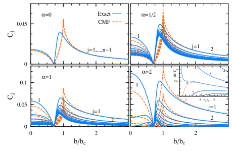
Figure 1: (Color online) Comparison between exact (solid lines) and CMF (dashed lines) results for the ground state concurrence $C_{j}$ of spin pairs with separation $j$ as a function of the transverse magnetic field $b$, for a long range $XY$ coupling $v^{\mu}(i-j)\propto v^{\mu}/|i-j|^{\alpha}$, with $\chi=v_{y}/v_{x}={\textstyle\frac{1}{2}}$ and $n=18$ spins. The concurrences vanish at the factorizing field $b_{s}=\sqrt{\chi}b_{c}$, where $b_{c}=v_{x}$ denotes the MF critical field. The inset depicts the reentry at high fields of the concurrence of distant pairs for $\alpha=2$.

The $\alpha=0$ case corresponds to the Lipkin model V.06 , where $v^{\mu}(j)=v^{\mu}/(n-1)$ and $\tilde{v}^{\mu}_{k}=v^{\mu}(n\delta_{k0}-1)/(n-1)$. In this case $C^{\pm}_{j}=C^{\pm}$ $\forall$ $j$, with $C^{\pm}<2/n$ KBI.00 due to the monogamy property CKW.00 . CMF is here quite accurate for all fields values away from $b_{c}$, providing the exact result for the rescaled concurrence $nC$ for large $n$ CMR.07 .

As $\alpha$ increases, CMF remains accurate for high fields $b\gtrsim 1.5b_{c}$, where the concurrence is correctly described by Eq. (31), i.e., $C_{j}\propto(v_{-}/b)/|j|^{\alpha}$. For sufficiently large $\alpha$ Eq. (31) actually predicts a weak reentry of the concurrence $C_{j}$ at strong fields for large separations $j$, since the last second order term in (31) will be negative and greater than the first order term for not too strong fields if $j$ is sufficiently large. This reentry is confirmed in the exact results for large separations, as seen here for $\alpha=2$ (inset of bottom right panel). CMF looses precision for low fields $|b|\lesssim b_{c}$, although for $\alpha\leq 1$ it is still quite reliable for $|b|<b_{s}$, where its accuracy increases as $j$ increases. Notice also that for $\alpha\leq 1$ we obtain for $n=18$ full range concurrence at all fields, whereas for $\alpha=2$ the concurrence becomes very short ranged at low fields ($j\leq 3$), being non-zero for large $j$ just in the vicinity of $b_{s}$ or at very strong fields, i.e., where the nearest neighbor concurrence becomes small, in agreement with the monogamy property. This behavior is qualitatively reproduced in CMF. Let us finally mention that for $\alpha=2$, results for the first few $C_{j}$ will remain stable as $n$ increases (as $\sum_{j}1/j^{\alpha}$ is in this case convergent), those of CMF remaining close to those depicted for $n=18$.

Fig. 2 depicts results for finite range couplings of constant strength, i.e., $v^{\mu}(j)=\frac{1}{2}v^{\mu}/L$ for $|j|\leq L$ and 0 otherwise (such that $\tilde{v}^{\mu}_{0}=v^{\mu}$), at the same anisotropy. For nearest neighbor coupling, which corresponds to the $\alpha\rightarrow\infty$ limit of the previous case, exact results for any finite $n$ and $T$ can be obtained with the Jordan-Wigner transformation LSM.61 plus parity projection RCM.08 . CMF is again confirmed to be accurate for high fields for both $j=1$ and $j=2$ (Eq. (32)), while for $|b|<b_{c}$ it provides only a qualitative agreement (with correct predictions like the full entanglement range in the vicinity of $b_{s}$), even though it is still reliable for standard observables like the spin correlation $\alpha_{x1}$ away from $b_{c}$ (inset in the upper left panel). The thermal behavior of $C_{j}$ is also correctly described by CMF away from $b_{c}$, as seen in the upper right panel, where exact results confirm the increase in the limit temperatures $T_{1}$ and $T_{2}$ for high fields as predicted by Eq. (34).

Nevertheless, the accuracy of CMF at low fields improves as soon as the range $L$ is increased, i.e., as $v^{\mu}(j)/v^{\mu}$ decreases. For instance, results at $b/b_{c}=0.1$ significantly improve already for $L\geq 2$, as seen in the bottom right panel, while for $L=3$ CMF is seen to provide the correct general picture except in the vicinity of $b_{c}$ (bottom left panel). In particular, the concurrence range for high fields is seen to be again twice the coupling range, in agreement with Eq. (31) (actually, for $j=6$ both the first and second order terms in Eq. (31) vanish for $\chi=1/2$ and $L=3$, and an expansion up to $O(v^{x}/b)^{3}$ is required, $C_{6}(b)$ being still positive in both CMF and the exact results). The splitting of the concurrences $C_{j}$ for $j=1,2,3$ is as well a second order effect.

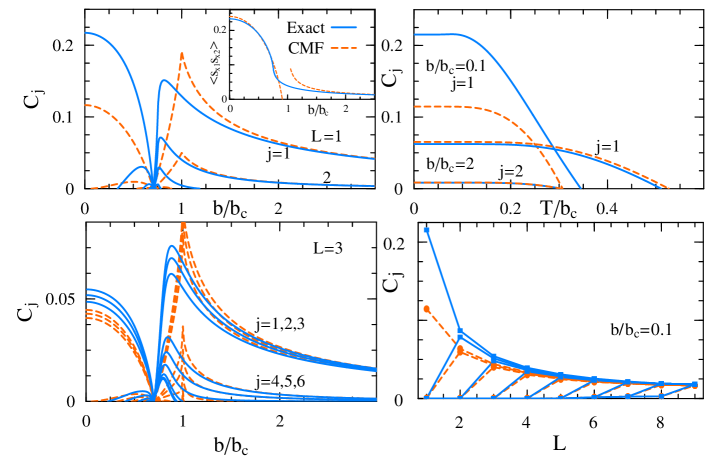
Figure 2: (Color online) Results for finite range $XY$ couplings at the same anisotropy $\chi=1/2$. Top panels depict the concurrence for nearest neighbor coupling ($L=1$) and $n=100$ spins, as a function of the transverse field at $T=0$ (left) and as a function of temperature at fixed fields (right). The inset depicts the spin correlation $\langle S_{x1}S_{x2}\rangle$ at $T=0$. Bottom: Results for interaction range $L$ and constant strength ($v^{\mu}(i-j)\propto v^{\mu}$ if $|i-j|\leq L$ and $0$ otherwise) for $n=18$ spins at $T=0$. The left panel corresponds to $L=3$ (third neighbor coupling) while the right panel depicts the concurrences $C_{j}$ as a function of the range $L$ at fixed low field.

IV Conclusions

We have examined a general MF+RPA treatment for describing composite systems with quadratic interactions at both zero and finite temperature, showing that it becomes particularly simple for finite translationally invariant systems with uniform mean fields. The approach is capable of reproducing the main features of the pairwise entanglement, for all pair separations, in cyclic spin 1/2 chains with anisotropic $XY$ couplings of different ranges, away from MF critical regions. It also provides the correct asymptotic behavior of the concurrence for strong fields, where it predicts interesting features like the possibility of a reentry of the pairwise concurrence for large separations, as well as an entanglement range which can be at most twice that of the interaction for finite range couplings, which were confirmed in the exact results. It also predicts the factorizing field and the full entanglement range in its immediate vicinity.

The method is specially suited for treating systems with high connectivity or long range interactions, where its accuracy improves. Let us remark that the individual components are in principle arbitrary in the present formalism. They could be also chosen as small arrays of coupled spins or subsystems treated exactly, leaving the RPA for the remaining interactions, a possibility which is currently under investigation and which could improve results for finite range couplings or dimer type chains. The extension to higher dimensions is as well straightforward.

J.M.M. and N.C. acknowledge support of CONICET, and R.R. of CIC, of Argentina.

References

- (1) D. Bohm and D. Pines, Phys. Rev. 92, 609 (1953).
- (2) P. Ping and P. Schuck, The nuclear Many-Body problem Springer (New York) (1980).
- (3) A.K. Kerman, S. Levit and T. Troudet, Ann. of Phys. (NY) 148, 436 (1983).
- (4) M.A. Nielsen and I. Chuang, Quantum Computation and Quantum Information, Cambridge Univ. Press (2000).
- (5) C.H. Bennett and D.P. DiVincenzo, Nature 404, 247 (2000).
- (6) T.J. Osborne, M.A. Nielsen, Phys. Rev. A 66, 032110 (2002).
- (7) G. Vidal, J.I. Latorre, E. Rico, A. Kitaev, Phys. Rev. Lett. 90, 227902 (2003).
- (8) L. Amico, R. Fazio, A. Osterloh and V. Vedral, Rev. Mod. Phys. 80, 517 (2008).
- (9) T. Kashiwa, Y. Ohnuki, and M. Susuki, Path Integral Methods, Oxford Univ. Press (1997).
- (10) U. Schollwöck, Rev. Mod. Phys. 77, 259 (2003).
- (11) F. Verstraete, J.I. Cirac, Phys. Rev. B 73 094423 (2006).
- (12) H. J. Lipkin, N. Meshkov, and A. J. Glick, Nucl. Phys. 62, 188 (1965).
- (13) J. Vidal, Phys. Rev. A 73 062318 (2006); S. Dusuel, J. Vidal, Phys. Rev. B 71, 224420 (2005).
- (14) N. Canosa, J.M. Matera, and R. Rossignoli, Phys. Rev. A 76 022310 (2007); J.M. Matera, R. Rossignoli, N. Canosa, Phys. Rev. A 78 012316 (2008).
- (15) J. Kurmann, H. Thomas, and G. Müller, Physica A 112, 235 (1982).
- (16) L. Amico et al, Phys. Rev. A 74, 022322 (2006).
- (17) R. Rossignoli, N. Canosa, J.M. Matera, Phys. Rev. A 77, 052322 (2008).
- (18) R. L. Stratonovich, Dokl. Akad. Nauk SSSR 115, 1097 (1957). J. Hubbard, Phys. Rev. Lett. 3, 77 (1959).
-
(19)
G. Puddu, P.F. Bortignon, and R. Broglia, Ann. Phys. (N.Y.)
206, 409 (1991).
H. Attias, Y. Alhassid, Nucl. Phys. A 625, 565 (1997). - (20) R. Rossignoli, N. Canosa, P. Ring, Phys. Rev. Lett. 80, 1853 (1998); Ann. of Phys. (NY) 275, 1 (1999).
- (21) E. Lieb, T. Schultz, and D. Mattis, Ann. of Phys. (NY) 16, 407 (1961).
- (22) S. Hill and W.K. Wootters, Phys. Rev. Lett. 78, 5022 (1997); W.K. Wootters, Phys. Rev. Lett. 80, 2245 (1998).
- (23) M. Koashi, V. Buzek, and N. Imoto, Phys. Rev. A 62, 050302(R) (2000).
- (24) V. Coffman, J. Kundu and W.K. Wootters, Phys. Rev. A 61 052306 (2000); T.J. Osborne and F. Verstraete, Phys. Rev. Lett. 96, 220503 (2006).