Geometric Ergodicity of Two–dimensional Hamiltonian systems with a Lennard–Jones–like Repulsive Potential

1. Introduction

Molecular dynamics simulation is among the most important and widely used tools in the study of molecular systems, providing fundamental insights into molecular mechanisms at a level of detail unattainable by experimental methods [AT87, Lea96, FS96, Sch02, Tuc10]. Usage of molecular dynamics spans a diverse array of fields, from physics and chemistry, to molecular and cellular biology, to engineering and materials science. Due to their size and complexity, simulations of large systems such as biological macromolecules (DNA, RNA, proteins, carbohydrates, and lipids) are typically performed under a classical mechanics representation. A critical requirement of such simulations is ergodicity, or convergence in the limit to the equilibrium (typically canonical) Boltzmann measure $\mu(d\mathbf{q},d\mathbf{p})=Z(\beta)^{-1}\mathrm{e}^{-\beta H(\mathbf{q},\mathbf{p})}d\mathbf{q}d\mathbf{p}$. Although ergodicity is commonly assumed, recently [CS08] showed that many commonly used deterministic dynamics methods for simulating the canonical (constant-temperature) ensemble fail to be ergodic. They also showed that introduction of a stochastic hybrid Monte Carlo (HMC) corrector guarantees ergodicity; however, HMC scales poorly with system dimension and is rarely used for macromolecules. [CS08] also show empirically that more commonly used stochastic Langevin dynamics [Pas94] appear to exhibit ergodic behavior, but were unable to provide rigorous proof.

The key difficulty in applying existing arguments [MSH02] is the appearance of singularities in the potential $U(\mathbf{q})$. Most modern molecular mechanics force fields [PCC⁺95, BBO⁺83, JTR88] take the form

$$U(\mathbf{q}) =\sum_{\rm bonds}K_{1}(r-r^{*})^{2}+\sum_{\rm angles}K_{2}(\theta-\theta^{*})^{2}+\sum_{\rm dihedrals}\frac{V_{n}}{2}[1+{\rm cos}(n\phi-\gamma)]$$

$$\qquad+\;\;\sum_{i<j}\left[\frac{A_{ij}}{r_{ij}^{12}}-\frac{B_{ij}}{r_{ij}^{6}}+\frac{q_{i}q_{j}}{\epsilon\,r_{ij}}\right]$$

Here the first three terms involve bond length, angle, and torsional energies; being bounded, these are easily handled. The difficulty arises from the non-covalent electrostatic and Van der Waals forces, the latter modeled by a Lennard-Jones potential, which give rise to singularities as two atoms in the system approach each other at close range.

In this paper we establish ergodicity of Langevin dynamics for a simple two-particle system involving a Lennard-Jones type potential. Moreover, we show that the dynamics is geometrically ergodic (i.e. has a spectral gap) and converges at a geometric rate. Geometric ergodicity is sufficient to imply existence of a central limit theorem for ergodic averages of functions $f$ with $\mathbf{E}_{\mu}(\left|f\right|^{2+\delta})<\infty$ for some $\delta>0$ [IL71], and also implies the existence of an exact sampling scheme [Ken04], although the latter need not be practical. Loosely, proving an ergodic result has two central ingredients. One provides continuity of the transition densities in total variation norm which ensures that transitions from nearby points behave similarly enough probabilistically, providing the basic mechanism of the probabilistic mixing/coupling. This is often expressed in a minorization condition (see Lemma 5.7). The other ingredient gives control of excursions towards infinity which ensures the existence of a stationary measure and guarantees that sufficient probabilistic mixing for an exponential convergence rate. The difficulty in a problem is typically one or the other.

As this paper was being accepted for publication, we became aware of two papers which prove results related to this paper; namely, [CG10, GS15]. The results are different in the cases where both apply. Here we prove exponential convergence to equilibrium from arbitrary initial data in variants of the total variation distance by building an optimal Lyapunov function. Consequently, our methods can handle weighted norms whose weight functions grow faster at infinity. In [CG10, GS15], the convergence of time averages is proven in $L^{2}$ when the system is started from equilibrium. In this sense, these results are together best characterized as mixing and make use in a critical way that the invariant measure is known as they build on the idea of Hypercoercivity. However, the scope of these two impressive papers, [CG10, GS15], is much larger. For example, they are able to handle the chain of interacting diffusions while we handle only two particles interacting currently with our methods.

In Section 2, we will see that in the current setting, basic existence of a stationary measure is trivial since the standard Gibbs measure built from the energy is invariant. Uniqueness of the stationary distribution follows from now standard results on hypoelliptic diffusions. However the control necessary to give a convergence rate or even convergence has previously been elusive. Our approach follows the established method of demonstrating the existence of a Lyapunov function and associated small set; however, construction of the Lyapunov function in the presence of a singular potential is non-trivial and our approach constitutes one of the major innovations of this paper. In many ways it builds on ideas in [HM09] and more obliquely is related to the ideas in [RBT02]. In both cases, time averaging of the instantaneous energy dissipation rate is used to build a Lyapunov function. We use similar ideas here. In a nutshell, as in [HM09] the technique consists of casting the behavior of the system as the energy heads to infinity as a problem with order one energy containing a small parameter equal to one over the original system’s energy. Then, classical stochastic averaging techniques are used to build a Lyapunov function. Though the solution is related to [HM09], the presentation of difficulties is quite different. In particular, we will see that extracting the asymptotic behavior is more difficult than [HM09] as our potentials do not strictly scale homogeneously. To overcome this we will use the idea of approximating the dynamics near the point at infinity from [AKM12, HM15a, HM15b] as well as techniques for joining together peicewise-defined Lyapunov functions in an analytically simple way from [HM15a, HM15b].

In Section 3, we state the main results of the paper which are derived from the existence of an appropriate Lyapunov function. Section 4 gives an overview of the construction of the Lyapunov function as well as some heuristic descriptions of its origin. More specifically in Section 4.2, we present some numerical experiments which show that our Lyapunov function is in some sense correct. In Section 4.3.1, we give a digestible overview of the basic ideas used in the construction while in Section 4.3.2, we give some indications of the relation between the ideas discussed in Section 4.3.1 and the ideas of hypocoercivity. In Section 4.3.3, we introduce the approximate dynamics which makes the analysis outlined in Section 4.3.1 feasible. The actual Lyapunov function is defined in Section 4.3.4 in terms of solutions of Poisson equations associated to the approximate dynamics introduced in Section 4.3.3. In Section 5, we give some consequences of the Lyapunov structure we have proven. In Section 6 and the Appendix, we give the missing details from the proof that the candidate function constructed is in fact a proper Lyapunov function. We conclude in Section 7 by briefly discussing the challenges of extending our results to larger systems and the case of a harmonically growing potential which is not covered by our results.

2. A Model Problem

Consider the two-particle Hamiltonian system $(\mathbf{Q},\mathbf{P})=\left((Q_{1},Q_{2}),(P_{1},P_{2})\right)$ with Hamiltonian

$$H_{0}(\mathbf{Q},\mathbf{P})=\frac{P_{1}^{2}}{2}+\frac{P_{2}^{2}}{2}+U(Q_{1}-Q_{2})$$

and interaction potential

$$U(Q)=\sum_{j=1}^{l}a_{j}|Q|^{\alpha_{j}}>0,$$ (1)

where $a_{j}\in\mathbb{R}$ with $a_{1},a_{l}>0$, and $\alpha_{1}>\cdots>\alpha_{l}$. We assume that $\alpha_{1}>2$ and $\alpha_{l}<0$ (otherwise no singularity exists). The dynamics of this system is given by

$$\dot{Q}_{i}=\frac{\partial H_{0}}{\partial P_{i}}\qquad\dot{P}_{i} =-\frac{\partial H_{0}}{\partial Q_{i}}\qquad\text{for $i=1,2$.}$$

If we force the system with a noise whose magnitude is scaled to balance dissipation so as to place the system at temperature $T$, then we arrive at the system of coupled SDEs

$$dq_{i} =p_{i}\,dt\qquad\text{for $i=1,2$}$$ (2)

$$dp_{1} =-U^{\prime}(q_{1}-q_{2})\,dt-\gamma p_{1}\,dt+\sigma dW_{1}(t)$$

$$dp_{2} =\;U^{\prime}(q_{1}-q_{2})\,dt-\gamma p_{2}\,dt+\sigma dW_{2}(t)$$

where the friction $\gamma>0$ and $\sigma^{2}=2\gamma T$. Define

$$\mathbb{S}\!\overset{\text{\tiny def}}{=}\!\Big{\{}(p_{1},q_{1},p_{2},q_{2}):q_{1}\neq q_{2}\Big{\}}.$$

We will prove in Corollary 5.4 that, if the initial conditions are in $\mathbb{S}$, then with probability one there exists a unique strong solution to (2) which is global in time and stays in $\mathbb{S}$.

We define the Markov semigroup by $(\mathcal{P}_{t}\phi)(\mathbf{p},\mathbf{q})\!\overset{\text{\tiny def}}{=}\!\mathbf{E}_{(\mathbf{p},\mathbf{q})}\phi(\mathbf{p}_{t},\mathbf{q}_{t})$ where $\mathbf{E}_{(\mathbf{p},\mathbf{q})}$ is the expected value starting from $(\mathbf{p},\mathbf{q})$ . This semigroup has a generator $\mathcal{L}_{0}$ given by

$$\mathcal{L}_{0}\;\!\overset{\text{\tiny def}}{=}\!\sum_{i=1,2}\frac{\partial H_{0}}{\partial p_{i}}\frac{\partial}{\partial q_{i}}-\frac{\partial H_{0}}{\partial q_{i}}\frac{\partial}{\partial p_{i}}-\gamma p_{i}\frac{\partial}{\partial p_{i}}+\gamma T\frac{\partial^{2}}{\partial p_{i}^{2}}\,.$$

Additionally $\mathcal{P}_{t}$ induces a dual action on $\sigma$-finite measures $\mu$ by acting on the left: $\mu\mathcal{P}_{t}$. A measure $\mu_{0}$ is a stationary measure of $\mathcal{P}_{t}$ if $\mu_{0}\mathcal{P}_{t}=\mu_{0}$. In our setting, this is equivalent to asking that $\mathcal{L}_{0}^{*}\rho_{0}=0$ where $\mu_{0}(d\mathbf{p},d\mathbf{q})=\rho_{0}(\mathbf{p},\mathbf{q})d\mathbf{p}\,d\mathbf{q}$.

It is a simple calculation to see that if

$$\rho_{0}(\mathbf{p},\mathbf{q})\,\!\overset{\text{\tiny def}}{=}\!\,Ce^{-H_{0}(\mathbf{p},\mathbf{q})/T}$$

for any $C$, then $\mathcal{L}_{0}^{*}\rho_{0}(\mathbf{p},\mathbf{q})=0$. Hence with this choice of $\rho_{0}$, $\mu_{0}$ as defined above is a stationary measure. However this measure is not normalizable to make a probability measure since it is only $\sigma$-finite. This stems from the fact that the Hamiltonian is translationally invariant in $\mathbf{q}$. To rectify his problem we will move to “center of mass” coordinates.

2.1. Reduction to Center of Mass Coordinates

Let $\tilde{q}=\frac{1}{2}(q_{1}-q_{2})$, $\tilde{p}=\frac{1}{2}(p_{1}-p_{2})$, $\bar{q}=\frac{1}{2}(q_{1}+q_{2})$, $\bar{p}=\frac{1}{2}(p_{1}+p_{2})$, $W=\frac{1}{2}(W_{1}-W_{2})$ and $B=\frac{1}{2}(W_{1}+W_{2})$. Then

$$d\bar{q}_{t} =\bar{p}_{t}\,dt$$ (3)

$$d\bar{p}_{t} =-\gamma\bar{p}_{t}\,dt+\sigma dB_{t}$$

$$d\tilde{q}_{t} =\tilde{p}_{t}\,dt$$

$$d\tilde{p}_{t} =-U^{\prime}(2\tilde{q}_{t})\,dt-\gamma\tilde{p}_{t}\,dt+\sigma dW_{t}$$

In these new coordinates, the system is described by variables $(\bar{q},\bar{p})$ tracking the position and momentum of the center of mass, and variables $(\tilde{q},\tilde{q})$ tracking the relative position and momentum of the particles within the center of mass frame. This change of coordinates simplifies our problem to two uncoupled Hamiltonian sub-problems. The center of mass $(\bar{q},\bar{p})$, has Hamiltonian

$$\bar{H}(\bar{q},\bar{p})\,\!\overset{\text{\tiny def}}{=}\!\,\frac{\bar{p}^{2}}{2}$$

which is the Hamiltonian of a free 1D particle, with corresponding invariant measure given by a Gaussian (for momentum $\bar{p}$) times 1D Lebesgue measure (for position $\bar{q}$). Note that $\bar{p}$ follows an Ornstein-Uhlenbeck process and hence converges exponentially quickly to its (Gaussian) stationary measure. The position $\bar{q}$ will diffuse through space like 1D Brownian motion and hence converges to Lebesgue measure.

The remaining two variables $(\tilde{q},\tilde{p})$ are also a Hamiltonian system with Hamiltonian

$$H(\tilde{q},\tilde{p})\,\!\overset{\text{\tiny def}}{=}\!\,\frac{\tilde{p}^{2}}{2}+U(2\tilde{q})\,.$$ (4)

which is a single particle interacting with a potential $U$ that is attractive towards the origin at large distances, and repulsive at short distance. So $(\tilde{q},\tilde{p})$ will have an invariant probability measure. However convergence of this system is more subtle; it possesses two difficulties stemming from the structure of the potential. First, since $U(Q)$ is singular at points, a strictly positive density does not exist everywhere in space. Second, there is no immediate candidate for a Lyapunov function. Overcoming this second obstacle will prove more difficult and will occupy the bulk of this paper.

3. Reduced system: main results

We now turn to the study of the two–dimensional Hamiltonian system described by (4). In this section, we also state the principal results on this reduced system.

Consider the two-dimensional deterministic Hamiltonian system with Hamiltonian

$$H(Q,P)\!\overset{\text{\tiny def}}{=}\!\frac{P^{2}}{2}+U(Q)$$

and hence dynamics

$$\dot{Q}_{t}=\frac{\partial H}{\partial P}(Q_{t},P_{t})=P_{t}\qquad\text{and}\qquad\dot{P}_{t} =-\frac{\partial H}{\partial Q}(Q_{t},P_{t})=-U^{\prime}(Q_{t})\,.$$

This system has only closed orbits, which lie completely in the upper half plane denoted by $\mathbb{H}=\{(Q,P)\in\mathbb{R}^{2}:Q>0\}$ provided the initial points lie in $\mathbb{H}$. To see this observe that when $|(Q,P)|\rightarrow\infty$, $H(Q,P)$ is well approximated by $\frac{1}{2}P^{2}+a_{1}Q^{\alpha_{1}}+a_{K}Q^{\alpha_{l}}$ which clearly has level sets that are closed, homotopically a circle, and lie completely in the upper half plane. (See Figure 1).

Figure 1. Level sets of $H(Q,P)=\eta$ for $\eta$ equals 1 (in blue), 2 (in green), and 4 (in red) where $H(Q,P)=\frac{1}{2}P^{2}+Q^{4}+\frac{1}{10}Q^{-2}$.

Addition of balanced noise and dissipation yields the associated stochastic system of interest. Namely, for positive temperature $T$, friction $\gamma$ and noise standard deviation $\sigma=\sqrt{2\gamma T}$, we have

$$dq_{t} =p_{t}\,dt$$ (5)

$$dp_{t} =-U^{\prime}(q_{t})\,dt-\gamma p_{t}\,dt+\sigma\,dW_{t}\,.$$

This Markov process has generator

$$\mathcal{L}\;=\frac{\partial H}{\partial p}\frac{\partial\ }{\partial q}-\frac{\partial H}{\partial q}\frac{\partial\ }{\partial p}-\gamma p\frac{\partial}{\partial p}+\gamma T\frac{\partial^{2}}{\partial p^{2}}$$

and as in the previous section a straightforward calculation shows that $\mu_{*}(dp\times dq)=\rho_{*}(q,p)dpdq$ is a stationary measure with

$$\rho_{*}(q,p)=Ce^{-H(q,p)/T},$$ (6)

since $\mathcal{L}^{*}\rho_{*}=0$. Unlike the stationary measure of the unreduced system, this measure can be normalized and made into a probability measure for an appropriate choice of $C$ (since $H$ is no longer translationally invariant).

In fact $\rho_{*}$ is the unique stationary measure of the system. To see this first observe that (5) is hypoelliptic and hence any weak solution to $\mathcal{L}^{*}\mu=0$ must locally have a smooth density with respect to Lebesgue measure. Since $\mu_{*}$ has an everywhere positive density with respect to Lebesgue measure it must therefore be the only stationary measure, since any stationary measure can be decomposed into its ergodic components all of which must have disjoint support. Uniqueness of the stationary measure is also a by-product of the exponential convergence given in Theorem 3.1 which is our main interest here.

To state this convergence result we need a distance between probability measures appropriate for our setting. To this end, for any $c\geq 0$ we define for $\phi:\mathbb{H}\rightarrow\mathbb{R}$ the weighted supremum-norm

$$\|\phi\|_{c}\!\overset{\text{\tiny def}}{=}\!\sup_{(q,p)\in\mathbb{H}}|\phi(q,p)|e^{-cH(q,p)}$$

and the weighted total-variation norm on signed measures $\nu$ with the property that $\nu(\mathbb{H})=0$ by

$$\|\nu\|_{c}\!\overset{\text{\tiny def}}{=}\!\sup_{\phi:\|\phi\|_{c}\leq 1}\int_{\mathbb{H}}\phi\,d\nu\,.$$

When $c=0$ this is just the standard total-variation norm. We define $\mathcal{M}_{c}(\mathbb{H})$ to be the set of probability measures $\mu$ on $\mathbb{H}$ with $\int_{\mathbb{H}}\exp(cH)d\mu<\infty$. Then we have the following convergence result.

Theorem 3.1.

For any $c\in(0,1/T)$, there exist positive constants $C$ and $D$ such that for any two probability measures $\mu_{1},\mu_{2}\in\mathcal{M}_{c}(\mathbb{H})$

$$\|\mu_{1}\mathcal{P}_{t}-\mu_{2}\mathcal{P}_{t}\|_{c}\leq Ce^{-Dt}\|\mu_{1}-\mu_{2}\|_{c}$$

for all $t\geq 0$. In particular the system has a unique invariant measure, which necessarily coincides with $\mu_{*}$ defined above, and to which the distribution of ($q_{t},p_{t})$ converges exponentially fast.

Our proof of Theorem 3.1 will follow the now standard approach of establishing the existence of an appropriate “small set” and a Lyapunov function [MT93a]. Similar to [MSH02], we will use a control argument coupled with hypoellipticity to establish the existence of a small set. While this is rather standard, the technique used to prove the existence of a Lyapunov function is less standard and one of the central contributions of this paper.

4. The Lyapunov function: Overview

4.1. Heuristics and motivating discussion

We wish to control motion out to infinity ($|(q,p)|\rightarrow\infty$) as well as in the neighborhood of the singularity ($q\rightarrow 0^{+}$). A standard route to obtaining such control is to find a Lyapunov function $V:\mathbb{H}\rightarrow(0,\infty)$ so that

$$dV(q_{t},p_{t})\leq-cV(q_{t},p_{t})dt+Cdt+dM_{t}$$ (7)

for some martingale $M_{t}$ and positive constants $c,C$ and such that $H\leq C_{0}V$ for some positive $C_{0}$. In particular, the fact that $V\rightarrow\infty$ as $q\rightarrow 0^{+}$ allows us to control the time spent near $q=0$.

The first reasonable choice for a Lyapunov function might be to try the Hamiltonian $H(q,p)$ itself. Using Itô’s formula, we see that

$$dH(q_{t},p_{t})=-\gamma p_{t}^{2}dt+\frac{\sigma^{2}}{2}dt+\sigma p_{t}dW_{t}\,.$$ (8)

However the function $(q,p)\mapsto p^{2}$ is not bounded below by $(q,p)\mapsto H(q,p)$ since the two functions are not comparable. This prevents us from obtaining the desired bound. If $U(q)$ only has positive powers of $q$ that are greater or equal to two, this deficiency can be partially overcome by considering $V(q,p)=H(q,p)+\gamma_{0}pq$. Then by picking $\gamma_{0}$ small enough, we can ensure that $\frac{1}{c}H\leq V\leq cH$ as $p^{2}+q^{2}\rightarrow\infty$ and that $\mathcal{L}V$ is bounded from above by a constant times $-V+C$ for some $C>0$. Hence $V$ is comparable to $H$ but satisfies the desired Lyapunov-function inequality (7). See [MSH02] for more on using this trick in this context.

Unfortunately this simple trick does not work in the presence of a singular repulsive term, as it does not yield the required bound for geometric ergodicity when $q$ approaches 0. This is necessary since the potential, and hence the transition density, behaves poorly near this point and uniform estimates are not easy (if even possible) to obtain. It is therefore reasonable to ask if there is a different choice other than $pq$ that will work yet is inspired by this example. Eventually, we will find an appropriate function $\Psi$ so that $V=H+\Psi$ works; to do so we will leverage a better understanding the dynamics at large energies. Moreover, this will allow us to learn a different way to understand the $pq$ correction than via the theory of hypocoercivity which it motivated. In Section 4.3.2, we will return to this example which is connected to the theory of hypocoercivity, which it partially inspired, and see how it fits into the approach we have developed.

With this example and its limitations in mind, we return to (8) and take a closer look at the dynamics. Looking at the right hand side, it is true that $p^{2}$ is not comparable to $H(q,p)$ at every given point $(q,p)$ in phase space. Yet if we really believe that the system settles down into equilibrium exponentially fast, the $-p^{2}$ term must lead to some “dissipation” of energy when the energy is large.

To see how dissipation arises, it is sufficient to analyze the stochastic dynamics at large energies, which is a regime in which we know something about the dynamics. To leading order in $H$ it will follow the deterministic dynamics with stochastic fluctuations of lower order. At high energy, the highest order part of the potential $U$ dominates.

For discussion purposes, we will assume for the moment that the potential $U:\mathbb{H}\rightarrow(0,\infty)$ has the simplified form

$$U(Q)=aQ^{\alpha}+bQ^{-\beta}$$ (9)

for some $a,b>0$ and $\alpha,\beta>0$ with $\alpha>2$. Later in this section, we will return to the problem when $U(Q)$ has the more general form (1). It will be convenient to introduce the following family of potentials indexed by a parameter $\epsilon\in[0,1]$

$$U_{\epsilon}(Q)=aQ^{\alpha}+bQ^{-\beta}\epsilon^{1+\frac{\beta}{\alpha}}.$$

Setting $\epsilon=1$ yields the original potential which we will continue to denote by $U$ without any subscript. The advantage provided by considering this family of potentials is that $U_{\epsilon}(Q)$ has the following homogeneous scaling property for $h>0$

$$U_{\epsilon}(h^{\frac{1}{\alpha}}Q)=hU_{\frac{\epsilon}{h}}(Q),$$ (10)

and this scaling property will lead to all of the scaling properties mentioned subsequently.

The orbits of the deterministic trajectories are given by the solution set of $H_{\epsilon}(Q,P)=\frac{1}{2}P^{2}+U_{\epsilon}(Q)=\eta$ for a given energy level $\eta>0$. This locus is topologically equivalent to a circle and hence setting

$$\varrho_{\epsilon}(Q,\eta)=\sqrt{2(\eta-U_{\epsilon}(Q))},$$ (11)

the orbit is given by the set $\{(Q,\varrho_{\epsilon}(Q,\eta)),(Q,-\varrho_{\epsilon}(Q,\eta)):Q\in[Q^{\epsilon}_{-}(\eta),Q^{\epsilon}_{+}(\eta)]\}$ where $Q^{\epsilon}_{+}(\eta)$ and $Q^{\epsilon}_{-}(\eta)$ are respectively the largest and smallest positive roots of $\eta-U_{\epsilon}(Q)=0$. Notice that model potential we are currently considering always has exactly two solutions to $\eta-U_{\epsilon}(Q)=0$.

We will see that the period of the orbit goes to zero as the energy goes to infinity. Hence at high energy the system will make many orbits in an instant of time and the average of $-P^{2}$ around the deterministic orbits will give a good idea of the dissipation asymptotically as the energy becomes large. We see that averaging $P^{2}$ around this deterministic trajectory gives by symmetry

$$\langle P^{2}\rangle_{\epsilon}(\eta)=2\int_{Q^{\epsilon}_{-}(\eta)}^{Q^{\epsilon}_{+}(\eta)}\varrho_{\epsilon}(Q,\eta)dQ\,;$$

and similarly that the period $\tau_{\epsilon}(\eta)$ of this orbit can be expressed as

$$\tau_{\epsilon}(\eta)=2\int_{Q^{\epsilon}_{-}(\eta)}^{Q^{\epsilon}_{+}(\eta)}\frac{1}{\varrho_{\epsilon}(Q,\eta)}dQ.$$

To make the idea of “large energy” more precise we consider the rescaling of phase space defined by the mapping $(Q,P)\mapsto(h^{\frac{1}{2}}P,h^{\frac{1}{\alpha}}Q)$ for a scale factor $h>0$. Under this map, the associated energy will essentially scale by a factor $h$ for large $h$. However this is not exactly correct since the other terms in the potential do not scale in the same fashion. However, in light of (10), by changing the value of $\epsilon$ we can relate a scaled Hamiltonian exactly with an unscaled Hamiltonian having $\epsilon=h^{-1}$; that is, since $H_{\epsilon}(Q,P)=\frac{1}{2}P^{2}+U_{\epsilon}(Q)$, we see that $H_{\epsilon}(h^{\frac{1}{\alpha}}Q,h^{\frac{1}{2}}P)=hH_{\frac{\epsilon}{h}}(Q,P)$. In other words, the scaled system behaves exactly like the unscaled system at a higher energy. If we define the average value of $P^{2}$ about an orbit as

$$\mathcal{A}_{\epsilon}(P^{2})(\eta)\!\overset{\text{\tiny def}}{=}\!\frac{\langle P^{2}\rangle_{\epsilon}(\eta)}{\tau_{\epsilon}(\eta)}$$ (12)

then we also see that $\mathcal{A}_{\epsilon}(P^{2})(h\eta)=h\mathcal{A}_{\frac{\epsilon}{h}}(P^{2})(\eta)$.

Summarizing, the average of $P^{2}$ around the deterministic orbit with energy $h\eta$ and $\epsilon=1$ is the same as $h$ times the average of $P^{2}$ around the deterministic orbit with energy $\eta$ and $\epsilon=h^{-1}$ for the simplified potential considered in this section. We will see later that this will hold for sufficiently large energy for the more general potential (1) as well. If we define,

$$\Lambda(\eta)\!\overset{\text{\tiny def}}{=}\!\mathcal{A}_{\frac{1}{\eta}}(P^{2})(1)$$ (13)

then $\mathcal{A}_{1}(P^{2})(\eta)=\eta\Lambda(\eta)$. Furthermore, observe that as $\epsilon\rightarrow 0$, the level sets under potential $U_{\epsilon}(Q)$ converge (Figure 2), and $\mathcal{A}_{\epsilon}(P^{2})(1)$ converges to a positive constant $\Lambda_{*}$ as $\epsilon\rightarrow 0$. As we will see later

$$\Lambda_{*}=\frac{\int_{0}^{\widetilde{Q}}\big{(}1-aQ^{\alpha}\big{)}^{\frac{1}{2}}dQ}{\int_{0}^{\widetilde{Q}}\big{(}1-aQ^{\alpha}\big{)}^{-\frac{1}{2}}dQ}=\frac{2\alpha}{\alpha+2}$$ (14)

where $\widetilde{Q}=a^{-\frac{1}{\alpha}}$. Notice that $\Lambda_{*}$ is independent of the value of $a$ and since $\alpha>2$, observe that $\Lambda_{*}\in(1,2)$.

Figure 2. Level sets of $H_{\epsilon}(Q,P)=1$ for $\epsilon$ equals 1 (blue) and 1/2.15 (green) where $H_{\epsilon}(Q,P)=\frac{1}{2}P^{2}+Q^{4}+\frac{1}{10}\epsilon^{\frac{3}{2}}Q^{-2}$ The dashed line is the level set of $\frac{1}{2}P^{2}+Q^{4}=1$ with $P\geq 0$ to which the level sets of $H_{\epsilon}(Q,P)=1$ converge as $\epsilon\rightarrow 0$.

Now since at high energy (i.e. $\eta\gg 1$), $\mathcal{A}_{1}(P^{2})(\eta)=\eta\Lambda(\eta)\approx\eta\Lambda_{*}$, it is reasonable to approximate (8) by

$$dH(t)\approx-\gamma\Lambda_{*}H(t)dt+\zeta\,dt+\sigma\sqrt{\Lambda_{*}H(t)}dW(t)$$ (15)

when $H(t)\gg 1$ where $\zeta>0$ is constant. Note that $\zeta$ is negligible for $H(t)\gg 1$. The martingale in (15) was chosen so that its quadratic variation would be the time average of the quadratic variation of the martingale in (8). In making this approximation, we are not claiming that there is averaging in the traditional asymptotic sense. Namely, there is a small parameter going to zero that causes the whole system to speed up and hence the instantaneous effect on the system is increasing in the limit of that averaged parameter. Rather, at high energy the system acts (after rescaling) increasingly like a system with order one energy and a rescaled parameter $\epsilon$. The rescaling also leads to a rescaling of time so that an order one time in the rescaled system represents an increasingly short time in the original system. Hence in a short interval of time at high energy, one sees the effect of many rotations of the system, making the averaged quantities just calculated a good approximation.

In spirit this approach is initially not unlike one used to show stability of queuing systems and stochastic algorithms [DW94, HKM02, Mey08]. There a discrete time (and possibly discrete space) stochastic system is shown to converge after rescaling to a deterministic ODE which can easily be shown to be stable. Here we also rescale but do so primarily to introduce a small parameter (one over the energy) and then use averaging the study this limiting ODE system with a small parameter.

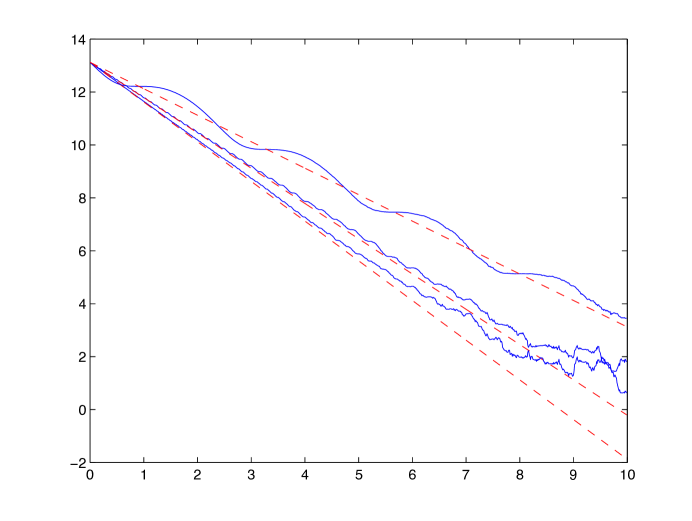
Figure 3. The first three plots are semi-log plots of energy versus time for the dynamics using the potential in (9) with $\alpha$ equal to 2 (upper most curve), 4 (middle curve), and 6 (lower most curve).The solid lines are numerical simulations and the dashed lines are the theoretical prediction made by (15).

Before making this intuition more formal in Section 4.3.3, we will present some numerical experiments which show that the above calculations capture the “truth” of what is going on. We will see the give the observed rate of energy dissipation at high energies.

4.2. Numerical explorations

The plots in Figure 3 compare the trajectory of the energy predicted by (15) and the energy trajectory obtained from a numerical simulation of (5) when both were started from the same initial high energy level. The model potential given in (9) was used with $\alpha\in\{2,4,6\}$ and $\beta=12$. Similar comparisons with $\beta$ equal to $2$ and $4$ were also made with nearly identical plots confirming essentially no dependence on $\alpha$ as predicted by our asymptotic theory.

Our theory only applies to the two cases $\alpha\in\{4,6\}$ since the theory requires $\alpha>2$. In these cases the agreement with the theory, shown with the dashed line, is quite good. One can see a small scale wiggle in the numerical curves. This is the effect of the periodic orbit. As the scaling theory predicts, the effect decreases as the energy increases since the scaling shows that period and the size of the fluctuations go to zero as the energy increases. When $\alpha=2$ our theory does not apply. Nonetheless, the trend given by dotted line is followed. However one sees that period and amplitude of the fluctuation is not going to zero which is also consistent with the scaling arguments predictions. The possibility of extending our theory to this boundary case is discussed in Section 7.

4.3. Definition of the Lyapunov function

Informed by the preceding discussion, we return to the idea of constructing a Lyapunov function $V$ of the form $V=H+\Psi$, where $\Psi$ is introduced to handle the singularity in $H$. The end result of this section, in particular, will be the definition of the corrector $\Psi$. First, however, we will take time to both motivate and explain how we arrived at this definition.

As discussed in Section 4.1, at high energy the system moves essentially around the deterministic orbit defined by the Hamiltonian flow. The average dissipative effect of each of these orbits is given by the average of the right hand side of (8) around one orbit. In the language of (12), this is $-\mathcal{A}_{1}(P^{2})(h)+\frac{\sigma^{2}}{2}$ if the energy equals $h$. To replace the $-p^{2}$ from (8) with $-\mathcal{A}_{1}(P^{2})(h)$, the theory of homogenization and averaging suggest the use of the “corrector” $\Psi$ defined by Poisson equation

$$\mathcal{H}\Psi(q,p)=\gamma(p^{2}-\mathcal{A}_{1}(P^{2})(H(p,q)))\,.$$

where $\mathcal{H}$ is the Liouville operator defined below. This can also be thought of as an “integration by parts” adapted to deterministic Hamiltonian dynamics in this setting, in the sense that

$$\int_{0}^{t}\gamma P_{s}^{2}\,ds=\Psi(P_{t},Q_{t})-\Psi(Q_{0},P_{0})+t\gamma\mathcal{A}_{1}(P^{2})(H(Q_{0},P_{0}))\,.$$

The first two terms on the righthand side of the equation above are boundary terms which control the fluctuations from the mean value.

This is the argument used in [HM09], where a succession of Poisson equations was employed to produce a sequence of correctors to reduce the fluctuations in various terms, achieving a function which was pointwise dissipative/coercive. In many ways the situation here is simpler than in [HM09] and the presentation clearer. However, we will see that a number of needed estimates proved elusive in this simple program as presented above. We will need to modify the above arguments by combining them with ideas the works [AKM12, HM15a, HM15b].

4.3.1. The basic idea

We begin by introducing the Liouville operator $\mathcal{H}$ associated with the deterministic dynamics given by

$$\mathcal{H}\!\overset{\text{\tiny def}}{=}\!P\partial_{Q}-U^{\prime}(Q)\partial_{P}.$$ (16)

Recalling that the full stochastic dynamics at large energies is approximately determined by the dynamics along $\mathcal{H}$, ideally we would like to pick the corrector $\Psi$ so that it satisfies the following two properties:

• $\Psi(Q,P)\in C^{2}(\mathbb{H}:\mathbb{R})$ and $\Psi$ satisfies the following PDE on $\mathbb{H}$

  $$(\mathcal{H}\Psi)(Q,P)=\gamma(P^{2}-\mathcal{A}_{1}(P^{2})(Q,P))$$ (17)

  where $\mathcal{A}_{\epsilon}(P^{2})(\eta)$ is the averaging operator defined by (12) discussed in Section 4.1 and we have introduced the slight abuse of notation

  $$\mathcal{A}_{\epsilon}(P^{2})(Q,P)\!\overset{\text{\tiny def}}{=}\!\mathcal{A}_{\epsilon}(P^{2})(H_{\epsilon}(Q,P))\,.$$

• $\Psi(Q,P)$ is “asymptotically dominated” by $H(Q,P)$ as $H(Q,P)\rightarrow\infty$, i.e., $\Psi$ satisfies

  $$\Psi(Q,P)=o(H(Q,P))\,\,\text{ as }\,\,H(Q,P)\rightarrow\infty.$$

In a moment, we will remark as to why we need to slightly weaken property (I) here, but for now let us assume that such a $\Psi$ satisfying (I) and (II) exists, as the essential structure of the argument that follows will still be employed.

Recall that that the generator $\mathcal{L}$ of the process defined by (5) can be written as

$$\mathcal{L}=\mathcal{H}-\gamma p\,\partial_{p}+\frac{\sigma^{2}}{2}\,\partial_{p}^{2}.$$

As mentioned above, we will choose the Lyapunov function $V$ to be $V=H+\Psi$. Since $\Psi$ satisfies the PDE in equation (17) of property (I), $\mathcal{A}_{1}(P^{2})(\eta)=\Lambda(\eta)\eta$ and $\mathcal{H}H=0$, we have that

$$dV(q_{t},p_{t})=(\mathcal{L}V)(q_{t},p_{t})dt+dM_{t},$$ (18)

where $M_{t}$ is a local martingale and

$$(\mathcal{L}V)(q,p)=-{\gamma}(\Lambda\circ H)(q,p)H(q,p)+\frac{\sigma^{2}}{2}-\gamma p\frac{\partial\Psi}{\partial p}(q,p)+\frac{\sigma^{2}}{2}\frac{\partial^{2}\Psi}{\partial p^{2}}(q,p)\,.$$ (19)

The first two terms of the right-hand side of (19) essentially coincide with (15); therefore, to realize our goal we would need to show that the remaining terms on the right-hand side are negligible at large energies.

To see intuitively why we expect these terms to be negligible at large energies, set $\beta=0$ in the potential $U(q)$ for simplicity and note that the operator $\mathcal{H}$ scales homogeneously of degree $\frac{1}{2}-\frac{1}{\alpha}$ under the transformation $(P,Q)\mapsto(h^{\frac{1}{2}}P,h^{\frac{1}{\alpha}}Q)$. Also, notice that the Hamiltonian $H$ scales homogeneously of degree $1$ under this transformation. Since the right hand side of (17) scales homogeneously of degree $1$ under the same transformation, we expect the corrector $\Psi$ to scale like $h^{\frac{1}{2}+\frac{1}{\alpha}}$. Since we assumed that $\alpha>2$, we see that (when $\beta=0$) $\Psi$ is dominated by $H$ at large energies just from this argument. Similarly, we expect $P\partial_{P}\Psi$ and $\partial^{2}_{P}\Psi$ to scale respectively like $h^{\frac{1}{2}+\frac{1}{\alpha}}$ and $h^{\frac{1}{\alpha}-\frac{1}{2}}$ under the same scaling, and hence are negligible as previously claimed.

When $\beta>0$, however, the situation is more complicated. A nice $C^{2}$ solution to (17) can still be found, yet determining its behavior at large energies is more delicate. For large energies where $q^{\alpha}$ dominates, the above analysis should still hold. For large energies where $q^{-\beta}$ dominates in $U(q)$, one can change the parameter $\epsilon$ in $U_{\epsilon}(q)$ from (10) to perform a similar scaling analysis for solutions of (17) with $U$ replaced by $U_{\epsilon}$. More precisely, if one defines $\mathcal{H}_{\epsilon}$ by (16) with $U^{\prime}(q)$ replaced by $U_{\epsilon}^{\prime}(q)$, then under the scaling transformation $(P,Q)\mapsto(h^{\frac{1}{2}}P,h^{\frac{1}{\alpha}}Q)$ we have that $\mathcal{H}_{\epsilon}$ transfroms to $h^{\frac{1}{2}-\frac{1}{\alpha}}\mathcal{H}_{\epsilon/h}$, which is analogous to how $\mathcal{H}$ transformed when $U(q)=q^{\alpha}$, except for the introduction of the parameter $\epsilon$. We then define $\Psi_{\epsilon}$ as the solution to (17) with $\mathcal{H}$ replaced by $\mathcal{H}_{\epsilon}$. Following the same logic as before, one sees that $\Psi_{\epsilon}$ transforms to $h^{\frac{1}{2}+\frac{1}{\alpha}}\Psi_{\epsilon/h}$ under $(P,Q)\mapsto(h^{\frac{1}{2}}P,h^{\frac{1}{\alpha}}Q)$. Similarly, $P\partial_{P}\Psi$ and $\partial^{2}_{P}\Psi$ transform to $h^{\frac{1}{2}+\frac{1}{\alpha}}P\partial_{P}\Psi_{\epsilon/h}$ and $h^{\frac{1}{\alpha}-\frac{1}{2}}\partial^{2}_{P}\Psi_{\epsilon/h}$, respectively. Hence we could repeat the same analysis if one had uniform control over the size of $\Psi_{\epsilon}$, $P\partial_{P}\Psi_{\epsilon}$ and $\partial^{2}_{P}\Psi_{\epsilon}$ as $\epsilon\rightarrow 0$. However, in all cases the rigorous extraction of the needed scaling of the original $\Psi$ or this family of solutions $\Psi_{\epsilon}$, and in particular the scaling of their derivatives, seems elusive. For this reason, we will modify the original PDE in (17) by introducing an approximate dynamics which will be asymptotically the same as the dynamics driven by the Hamiltonian but which will scale exactly homogeneously in the spirit of the previous paragraph. This will allow us to control the needed terms but it will come with a cost. That is, the resulting solution $\Psi$ will only be globally continuous and not globally $C^{2}$. It will however be piecewise $C^{2}$ and the ideas from [HM15a, HM15b] will be exploited to nonetheless prove $H+\Psi$ is a Lyapunov function for the time $t$ dynamics.

4.3.2. The relationship to the “$pq$” trick and Hypocoercivity

We now make a small digression and return to the “trick” used in the non-singular case of adding $\gamma_{0}pq$ for some choice of positive $\gamma_{0}$ as discussed in Section 4.1. In light of the construction used in this paper, it is interesting to ask if $\gamma_{0}pq$ is the solution of an appropriate Poisson equation of the problem with a potential $U(q)=q^{2n}/(2n)$, since this potential represents the behavior at infinity of the class of potentials for which that construction is used. We begin by observing that for the corresponding Liouville operator $\mathcal{H}$ one has

$$\mathcal{H}(pq)=p^{2}-q^{2n}=(1+n)p^{2}-np^{2}-q^{2n}=(1+n)p^{2}-2nH(p,q).$$

Hence multiplying by $\frac{\gamma}{1+n}$ and calculating that $\mathcal{A}(p^{2})(q,p)=\frac{2n}{n+1}H(q,p)$, we see that $\Psi(q,p)=\frac{\gamma}{1+n}pq$ is a solution to

$$(\mathcal{H}\Psi)(q,p)=\gamma p^{2}-\gamma\mathcal{A}(p^{2})(q,p)\,.$$

Hence this “trick” is exactly a version of the ideas in this paper, namely solving the correct, asymptotically relevant Poisson equation. It would be interesting to understand how this point of view fits together with the ideas contained in the theory of hypocoercivity as developed by C. Villani [Vil09] and subsequent authors [Bau13, DMS15, GS15, GS16].

4.3.3. The approximate dynamics

Rather than using the trajectories defined by the full Hamiltonian $H$ to build the corrector $\Psi$ via the method of characteristics, we will use the trajectories defined by a “piecewise Hamiltonian”. This has the advantage of simplifying, yet capturing the dynamics at large energies in various regions in the state space $\mathbb{H}$. This, in particular, will allow for easier analysis of our chosen corrector, as the PDEs satisfied by $\Psi$ locally in various regions in $\mathbb{H}$ will be far simpler than the equation (17) in property (I).

To introduce the approximate dynamics, recall that

$$H(Q,P)=\frac{P^{2}}{2}+U(Q)=\frac{P^{2}}{2}+\sum_{i=1}^{l}a_{i}Q^{\alpha_{i}}$$

where $\alpha_{1}>2,a_{1}>0,a_{l}>0$, $\alpha_{l}<0$ and

$$\alpha_{1}>\alpha_{2}>\cdots>\alpha_{l}.$$

Because two parts in $U(Q)$ will play a special role throughout the rest of the paper, we let $\alpha_{1}=\alpha$, $a_{1}=a$, $\alpha_{l}=-\beta$, $a_{l}=b$ for simplicity. For $(Q,P)\in\mathbb{H}$ let

$$K(Q,P)=\frac{P^{2}}{2}+bQ^{-\beta}\,\,\text{ and }\,\,J(Q,P)=\frac{P^{2}}{2}+aQ^{\alpha},$$ (20)

and for $\xi_{*},h_{*}>0$ define the following regions in the state space $\mathbb{H}$:

$$\mathcal{S}_{1}(\xi_{*},h_{*}) =\{(Q,P)\in\mathbb{H}\,:\,P^{2}Q^{\beta}\leq\xi_{*}^{2},\,Q<1,K(Q,P)\geq k(h_{*})\}$$

$$\mathcal{S}_{2}(\xi_{*},h_{*}) =\{(Q,P)\in\mathbb{H}\,:\,P^{2}Q^{\beta}\geq\xi_{*}^{2},P^{2}Q^{-\alpha}\geq\xi_{*}^{2},\,H(Q,P)\geq h_{*}\}$$

$$\mathcal{S}_{3}(\xi_{*},h_{*}) =\{(Q,P)\in\mathbb{H}\,:\,P^{2}Q^{-\alpha}\leq\xi_{*}^{2},\,Q>1,\,J(Q,P)\geq j(h_{*})\}$$

where $k(h)$ and $j(h)$ are boundary functions to be introduced momentarily. Both of the parameters $\xi_{*},h_{*}$ should be thought of as large, and we will see soon that $k(h),j(h)\approx h$ for $h>0$ large. The parameter $\xi_{*}>0$ will be increased at several instances throughout the paper. Moreover, we will often choose the parameter $h_{*}$ to depend on $\xi_{*}$.

To help motivate the regions above, observe that as $H(Q,P)\rightarrow\infty$ with $(Q,P)\in\mathcal{S}_{1}(\xi_{*},h_{*})$ we have

$$H(Q,P)=Q^{-\beta}\bigg{[}\frac{P^{2}Q^{\beta}}{2}+b+o(1)\bigg{]}=K(Q,P)+Q^{-\beta}o(1)$$

and as $H(Q,P)\rightarrow\infty$ with $(Q,P)\in\mathcal{S}_{3}(\xi_{*},h_{*})$

$$H(Q,P)=Q^{\alpha}\bigg{[}\frac{P^{2}Q^{-\alpha}}{2}+a+o(1)\bigg{]}=J(Q,P)+Q^{\alpha}o(1).$$

Since $P^{2}Q^{\beta}$ is bounded on $\mathcal{S}_{1}(\xi_{*},h_{*})$ and $P^{2}Q^{-\alpha}$ is bounded on $\mathcal{S}_{3}(\xi_{*},h_{*})$, this calculation suggests that we should take the approximate dynamics in $\mathcal{S}_{1}(\xi_{*},h_{*})$ to be the dynamics determined by the Hamiltonian $K(Q,P)$. Similarly in $\mathcal{S}_{3}(\xi_{*},h_{*})$, we should take the approximate dynamics to be the dynamics determined by the Hamiltonian $J(Q,P)$. The region $\mathcal{S}_{2}(\xi_{*},h_{*})$ corresponds to an asymptotically insignificant piece of the dynamics at large energies when $\xi_{*}$ is also large, and therefore should serve merely as a “transition zone” between two other regimes, $\mathcal{S}_{1}(\xi_{*},h_{*})$ and $\mathcal{S}_{3}(\xi_{*},h_{*})$. This, in particular, suggests that we maintain the dynamics determined by $H$ in the region $\mathcal{S}_{2}(\xi_{*},h_{*})$.

Remark 4.1.

It is also instructive to understand how the analogous regions for $\mathcal{H}_{\epsilon}$ transform under the scaling $(P,Q)\mapsto(h^{\frac{1}{2}}P,h^{\frac{1}{\alpha}}Q)$. If in the regions $\mathcal{S}_{i}$ we replace $P^{2}Q^{\beta}$ by $P^{2}Q^{\beta}\epsilon^{-1-\frac{\beta}{\alpha}}$, this then defines correct regions $\mathcal{S}_{i}^{\epsilon}$ corresponding to $\mathcal{H}_{\epsilon}$ (ignoring the truncation for small $H$ for the moment). Notice that the boundary between $\mathcal{S}_{3}^{\epsilon}$ and $\mathcal{S}_{2}^{\epsilon}$ would remain unchanged as $\epsilon\rightarrow 0$ yet the boundary between $\mathcal{S}_{1}^{\epsilon}$ and $\mathcal{S}_{2}^{\epsilon}$ will collapse towards the $q=0$ axis. Hence as $\epsilon\rightarrow 0$, the region $\mathcal{S}_{1}^{\epsilon}$ becomes a vanishingly small part of the phase space. Furthermore by making $\xi_{*}$ large we can decrease the importance of the dynamics in $\mathcal{S}_{2}^{\epsilon}$ by making this region smaller. Thus we expect only the dynamics in region $\mathcal{S}_{3}^{\epsilon}$ to be relevant asymptotically. In $\mathcal{S}_{3}^{\epsilon}$, the potential $U_{\epsilon}(q)$ is dominated by $aQ^{\alpha}$ as $\epsilon\rightarrow 0$ uniformly and we expect the dynamics governed by the Hamiltonian $J$ defined above to dominate. We will see that all of these predictions hold and that they are behind all of the construction on which we now embark.

To define the approximate dynamics precisely, we need some additional notation. For $h_{0}=h_{0}(\xi_{*})>0$ large enough and $h\geq h_{0}$, let $(Q_{1},P_{1})=(Q_{1}(\xi_{*},h),P_{1}(\xi_{*},h))\in\mathcal{S}_{1}(\xi_{*},h_{0})$ satisfy

$$H(Q_{1},P_{1}) =h,\,\,P_{1}^{2}=\xi_{*}^{2}Q_{1}^{-\beta},\,\,P_{1}>0$$

and $(Q_{3},P_{3})=(Q_{3}(\xi_{*},h),P_{3}(\xi_{*},h))\in\mathcal{S}_{3}(\xi_{*},h_{0})$ satisfy

$$H(Q_{3},P_{3}) =h,\,\,P_{3}^{2}=\xi_{*}^{2}Q_{3}^{\alpha},\,\,P_{3}>0.$$

From the asymptotic observations made above, we note that as $h\rightarrow\infty$

$$Q_{1}^{-\beta}\bigg{[}\frac{\xi^{2}_{*}}{2}+b+o(1)\bigg{]}=h\,\,\text{ and }\,\,Q_{3}^{\alpha}\bigg{[}\frac{\xi_{*}^{2}}{2}+a+o(1)\bigg{]}=h.$$

Now, for $h\geq h_{0}$, $h_{0}=h_{0}(\xi_{*})>0$ large enough, define $k(h),j(h)>0$ by

$$k(h)=h-\sum_{i=1}^{l-1}a_{i}Q_{1}^{\alpha_{i}},\qquad j(h)=h-\sum_{i=2}^{l}a_{i}Q_{3}^{\alpha_{i}}$$

and notice that

$$\lim_{h\rightarrow\infty}h^{-1}k(h)=\lim_{h\rightarrow\infty}h^{-1}j(h)=1.$$

By perhaps again increasing $h_{0}$ if necessary, also observe that for all $i\neq j$

$$\text{interior}(\mathcal{S}_{i}(\xi_{*},h_{0}))\cap\text{interior}(\mathcal{S}_{j}(\xi_{*},h_{0}))=\emptyset.$$

Setting

$$\mathcal{S}_{i}^{+}(\xi_{*},h_{0}) =\mathcal{S}_{i}(\xi_{*},h_{0})\cap\{(Q,P)\in\mathbb{H}\,:\,P\geq 0\}$$

$$\mathcal{S}_{i}^{-}(\xi_{*},h_{0}) =\mathcal{S}_{i}(\xi_{*},h_{0})\cap\{(Q,P)\in\mathbb{H}\,:\,P\leq 0\},$$

with this choice of $h_{0}$ we have sketched the regions $S_{j}(\xi_{*},h_{0})$ in Figure 4.

Figure 4. The regions $\mathcal{S}_{i}$, $i=1,2,3,4$, are plotted above along with the form of $\Psi$ in each region. The rotation along a cycle $\Gamma(h)$ for the approximate dynamics is in the counterclockwise direction. Thus boundary contributions $\overline{\Psi}_{i}^{\pm}$ accumulate in the clockwise direction. The specific choice of $\Psi$ was made so that $\Psi(Q,0)=0$ to exploit the symmetry in the problem. Also note that, in light of Remark 4.1, we expect for large energy and large $\xi_{*}$ that only the dynamics in the region $\mathcal{S}_{3}$ will be relevant.

We can now define the approximate dynamics. For simplicity, set $\mathcal{S}_{i}=\mathcal{S}_{i}(\xi_{*},h_{0})$, $\mathcal{S}_{i}^{\pm}=\mathcal{S}_{i}^{\pm}(\xi_{*},h_{0})$ and $\mathbb{H}_{h_{0}}=\bigcup\mathcal{S}_{i}$.

Definition 4.2 (The Approximate Dynamics).

For $(Q,P)\in\mathbb{H}_{h_{0}}$, the approximate dynamics started from $(Q,P)$ is the solution of the differential equation

$$(Q_{t},P_{t})=(Q,P)+\int_{0}^{t}X(Q_{s},P_{s})\,ds$$

where $X:\mathbb{H}_{h_{0}}\rightarrow\mathbb{R}^{2}$ is given by

$$X(Q,P)=\begin{cases}(P,b\beta Q^{-\beta-1})&\text{ if }\,(Q,P)\in\mathcal{S}_{1}\setminus\mathcal{S}_{2}^{+}\\ (P,-U^{\prime}(Q))&\text{ if }\,(Q,P)\in\mathcal{S}_{2}^{+}\setminus\mathcal{S}_{3}\\ (P,-a\alpha Q^{\alpha-1})&\text{ if }(Q,P)\in\mathcal{S}_{3}\setminus\mathcal{S}_{2}^{-}\\ (P,-U^{\prime}(Q))&\text{ if }\,(Q,P)\in\mathcal{S}_{2}^{-}\setminus\mathcal{S}_{1}\end{cases}.$$

One can check that for initial conditions $(Q,P)\in\mathbb{H}_{h_{0}}$, the approximate dynamics started from $(Q,P)$ has a unique solution with a corresponding continuous solution curve $\Gamma(h)$, where $H(Q,P)=h$, given by the union of the following curves

$$\Gamma_{1}(h) =\{(Q,P)\in\mathcal{S}_{1}\,:\,K(Q,P)=k(h)\}$$

$$\Gamma_{2}(h) =\{(Q,P)\in\mathcal{S}_{2}\,:\,H(Q,P)=h\}$$

$$\Gamma_{3}(h) =\{(Q,P)\in\mathcal{S}_{3}\,:\,J(Q,P)=j(h)\}.$$

4.3.4. Poisson equations and $\Psi$

Using the approximate dynamics, we will now define the corrector $\Psi$. We begin by defining the transport operators corresponding to flow generated by the approximate dynamics defined above. In other words, they are the first order differential operators whose characteristics correspond to the approximate dynamics. Defining the operators $\mathcal{K}$ and $\mathcal{J}$ by

$$\mathcal{K} \!\overset{\text{\tiny def}}{=}\!P\partial_{Q}+\beta bQ^{-\beta-1}\partial_{Q}$$

$$\mathcal{J} \!\overset{\text{\tiny def}}{=}\!P\partial_{Q}-\alpha aQ^{\alpha-1}\partial_{Q}.$$

we see that transport generated by the operator $\mathcal{K}$ corresponds to the flow of the approximate dynamics in $\mathcal{S}_{1}\setminus\mathcal{S}_{1}\cap\mathcal{S}_{2}^{+}$ while the transport generated by the operator $\mathcal{J}$ corresponds to the approximate dynamics in $\mathcal{S}_{3}\setminus\mathcal{S}_{2}^{-}\cap\mathcal{S}_{3}$. We recall that in the remaining regions in $\mathbb{H}_{h_{0}}$, the dynamics is that determined by the full Liouville operator $\mathcal{H}$.

For $h\geq h_{0}$ and $l=1,2,3$, we let $G_{l}(h)$ denote the total time spent by the approximate dynamics in $\mathcal{S}_{l}$ during one complete cycle on $\Gamma(h)$, and define $T(h)=\sum_{j=1}^{3}G_{l}(h).$ For $l=1,2,3$ and $h\geq h_{0}$, we let $F_{l}(h)$ be given by

$$F_{l}(h) \!\overset{\text{\tiny def}}{=}\!\int_{0}^{T(h)}\mathbf{1}_{\mathcal{S}_{l}}(Q_{s},P_{s})P_{s}^{2}\,ds$$

where in the above $\mathbf{1}_{\mathcal{S}_{l}}$ denotes the indicator function on $\mathcal{S}_{l}$, $(Q_{s},P_{s})$ corresponds to the coordinates of the approximate dynamics, and we are taking as our initial condition any point $(Q_{0},P_{0})$ belonging to $\Gamma(h)$. For positive parameters $c_{l}^{+}$ and $c_{l}^{-}$, $l=1,2,3$, and $h\geq h_{0}$, we define the weighted averages $\mathcal{A}_{+}(h)$ and $\mathcal{A}_{-}(h)$ by

$$\mathcal{A}_{\pm}(h)\!\overset{\text{\tiny def}}{=}\!\frac{\sum_{i=1}^{3}c_{i}^{\pm}F_{i}(h)}{\sum_{i=1}^{3}c_{i}^{\pm}G_{i}(h)}.$$ (21)

Remark 4.3.

Observe that $\mathcal{A}_{\pm}(h)$ are slight modifications of the average $\mathcal{A}_{1}(P^{2})(h)$ of $P^{2}$ over one cycle of the deterministic dynamics defined by the full Hamiltonian $H$. More precisely, they are weighted versions (with weights $c_{l}^{\pm}$) of the average of $P^{2}$ over one cycle of the approximate dynamics. Later we will see that for every $\epsilon>0$ there exists $\xi_{*}>0$ large enough such that for all $h\geq h_{0}=h_{0}(\xi_{*})$ large enough

$$1-\epsilon\leq\frac{\mathcal{A}_{1}(P^{2})(h)}{\mathcal{A}_{\pm}(h)}\leq 1+\epsilon.$$

More specifically, we will see that the asymptotically dominant part of $\mathcal{A}_{\pm}(h)$ is $c_{3}^{\pm}F_{3}(h)/c_{3}^{\pm}G_{3}(h)=F_{3}(h)/G_{3}(h)$; that is, the dominant contribution to the dissipation at large energies comes from region $\mathcal{S}_{3}$. We will need these slight modifications and the parameters $c_{l}^{\pm}$ to ensure that $\Psi$ defined below is smooth enough to apply Peskir’s extension of Itô’s formula [Pes07] and to deal with the signs of the local time contributions in $d\Psi(q_{t},p_{t})$ arising because $\Psi$ will not quite be globally $C^{2}$.

Just like the original dynamics determined by the full Liouville operator $\mathcal{H}$, the function $\Psi$ will be broken into several pieces. To introduce them, first recall the definitions of $j(h)$ and $k(h)$ introduced after Remark 4.1 and note that, by increasing $h_{0}$ if necessary, the functions

$$j:[h_{0},\infty)\rightarrow[j(h_{0}),\infty),\,\,k:[h_{0},\infty)\rightarrow[k(h_{0}),\infty)$$

are twice continuously differentiable with twice continuously differentiable inverse functions

$$j^{-1}:[j(h_{0}),\infty)\rightarrow[h_{0},\infty),\,\,k^{-1}:[k(h_{0}),\infty)\rightarrow[h_{0},\infty).$$

Moreover, it can be shown by implicit differentiation of $Q_{1}(h)$ and $Q_{3}(h)$ with respect to $h$ that the inverse functions satisfy

$$\lim_{h\rightarrow\infty}(h^{-1}j^{-1}(h)) =\lim_{h\rightarrow\infty}(h^{-1}k^{-1}(h))=1$$ (22)

$$\lim_{h\rightarrow\infty}(j^{-1})^{\prime}(h) =\lim_{h\rightarrow\infty}(k^{-1})^{\prime}(h)=1$$ (23)

$$\lim_{h\rightarrow\infty}|h(j^{-1})^{\prime\prime}(h)| =\lim_{h\rightarrow\infty}|h(k^{-1})^{\prime\prime}(h)|=0.$$ (24)

We let $\Psi_{1}^{+}$ and $\Psi_{2}^{-}$ be defined on $\mathcal{S}_{1}$ as the solutions of the following boundary-value PDEs

$$\begin{cases}&(\mathcal{K}\Psi_{1}^{\pm})(Q,P)=\gamma c_{1}^{\pm}\big{(}P^{2}-\mathcal{A}_{\pm}(k^{-1}(K))\big{)}\\ &\Psi_{1}^{\pm}(Q,P)=0\,\,\text{ for }P^{2}Q^{\beta}=\xi_{*}^{2},\,P>0\end{cases}$$ (25)

where $K=K(Q,P)$ is as in (20). Define $\Psi_{2}^{+}$ and $\Psi_{2}^{-}$ on $\mathcal{S}_{2}$ by

$$\begin{cases}&(\mathcal{H}\Psi_{2}^{+})(Q,P)=\gamma c_{2}^{+}\big{(}P^{2}-\mathcal{A}_{+}(H)\big{)}\\ &\Psi_{2}^{+}(Q,P)=0\,\,\text{ for }P^{2}Q^{-\alpha}=\xi_{*}^{2},P>0.\end{cases}$$ (26)

and

$$\begin{cases}&(\mathcal{H}\Psi_{2}^{-})(Q,P)=\gamma c_{2}^{-}\big{(}P^{2}-\mathcal{A}_{-}(H)\big{)}\\ &\Psi_{2}^{-}(Q,P)=0\,\,\text{ for }P^{2}Q^{\beta}=\xi_{*}^{2},P<0\end{cases}.$$ (27)

Lastly, for $(Q,P)\in\mathcal{S}_{3}$ define $\Psi_{3}^{+}$ and $\Psi_{3}^{-}$ as the solutions of

$$\begin{cases}&(\mathcal{J}\Psi_{3}^{\pm})(Q,P)=\gamma c_{3}^{\pm}\big{(}P^{2}-\mathcal{A}_{\pm}(j^{-1}(J))\big{)}\\ &\Psi_{3}^{\pm}(Q,P)=0\,\,\text{ for }P^{2}Q^{-\alpha}=\xi_{*}^{2},P<0\end{cases}$$ (28)

where $J=J(Q,P)$ is as in (20).

Remark 4.4.

At this point it is helpful to compare the righthand sides of the equations above with the righthand side of the equation (17) in property (I). Because $k^{-1}(K)$ and $j^{-1}(J)$ are asymptotically equivalent to $H$ in, respectively, $\mathcal{S}_{1}$ and $\mathcal{S}_{3}$, the only noticeable difference between the two is the presence of the parameters $c_{l}^{\pm}$. However as we will see later, we will be able to choose $c_{l}^{\pm}\leq 1$, $i=1,2,3$, arbitrarily close to $1$. Therefore, due to the asymptotic formula for $\mathcal{A}_{\pm}$ discussed in the previous remark, the equations satisfied by $\Psi_{i}^{\pm}$ approximate, up to a small constant, the equation in (I) when $H\rightarrow\infty$. We will see that this constant can be made arbitrarily small by first picking the boundary parameter $\xi_{*}>0$ large enough.

Because we have defined $\Psi_{i}^{\pm}$ using zero boundary conditions and $\Psi_{i}^{\pm}\neq 0$ on the other boundary in its region of definition, we cannot (as may be suggested by the above) by fixing a $+$ or $-$ define our corrector $\Psi$ to simply be $\Psi_{i}^{\pm}$ on $\mathcal{S}_{i}$. In particular, although we will see that each $\Psi_{i}^{\pm}$ is $C^{2}$ on $\mathcal{S}_{i}^{\pm}$, such a choice would mean that $\Psi$ is not globally continuous.

To see how to obtain the desired global continuity, let $g_{l}(Q,P)$, $l=1,2,3$, be the first exit time of the approximate dynamics from $\mathcal{S}_{l}$ started from $(Q,P)\in\mathcal{S}_{l}(\xi_{*},h_{0})$ and for $(Q,P)\in\mathcal{S}_{l}$ define

$$f_{l}(Q,P)\!\overset{\text{\tiny def}}{=}\!\int_{0}^{g_{l}(Q,P)}P_{s}^{2}\,ds$$

where again we recall that $P_{s}$ is the momentum coordinate of the approximate dynamics. Applying the method of characteristics to solve equations (25)-(26) produces the following expressions for $\Psi_{i}^{\pm}(Q,P)$:

$$\Psi_{1}^{\pm}(Q,P) =\gamma c_{1}^{\pm}\big{(}\mathcal{A}_{\pm}(k^{-1}(K))g_{1}(Q,P)-f_{1}(Q,P)\big{)}$$

$$\Psi_{2}^{\pm}(Q,P) =\gamma c_{2}^{\pm}\big{(}\mathcal{A}_{\pm}(H)g_{2}(Q,P)-f_{2}(Q,P)\big{)}$$

$$\Psi_{3}^{\pm}(Q,P) =\gamma c_{3}^{\pm}\big{(}\mathcal{A}_{\pm}(j^{-1}(J))g_{3}(Q,P)-f_{3}(Q,P)\big{)}$$

where $H=H(Q,P)=\frac{P^{2}}{2}+U(Q)$, $K=K(Q,P)=\frac{P^{2}}{2}+bQ^{-\beta}$ and $J=J(Q,P)=\frac{P^{2}}{2}+aQ^{\alpha}$. Hence for $(Q,P)\in\mathcal{S}_{i}\cap\Gamma(h)$, the value of $\Psi_{i}^{\pm}(Q,P)$, $i=1,2,3,4$, on the boundary where it is nonzero is given by

$$\overline{\Psi}_{1}^{\pm}(h) \!\overset{\text{\tiny def}}{=}\!\gamma c_{1}^{\pm}\big{(}\mathcal{A}_{\pm}(h)G_{1}(h)-F_{1}(h)\big{)}$$

$$\overline{\Psi}_{2}^{\pm}(h) \!\overset{\text{\tiny def}}{=}\!\frac{\gamma}{2}c_{2}^{\pm}\big{(}\mathcal{A}_{\pm}(h)G_{2}(h)-F_{2}(h)\big{)}$$ (29)

$$\overline{\Psi}_{3}^{\pm}(h) \!\overset{\text{\tiny def}}{=}\!\gamma c_{3}^{\pm}\big{(}\mathcal{A}_{\pm}(h)G_{3}(h)-F_{3}(h)\big{)}.$$

Remark 4.5.

Recall that for $h\geq h_{0}$, $G_{l}(h)$ denotes the total time spent by the approximate dynamics in $\mathcal{S}_{l}$ during one complete cycle on $\Gamma(h)$, and

$$F_{l}(h)=\int_{0}^{T(h)}\mathbf{1}_{\mathcal{S}_{l}}(Q_{s},P_{s})P_{s}^{2}\,ds$$

where $T(h)=G_{1}(h)+G_{2}(h)+G_{3}(h)$ is the time to complete one cycle. Hence the factor of $\frac{1}{2}$ appears on the righthand side of the expression for $\overline{\Psi}_{2}^{\pm}(h)$ above by symmetry since only one half of the trajectory in $\mathcal{S}_{2}$ is traversed starting in either $\mathcal{S}_{2}^{+}$ or $\mathcal{S}_{2}^{-}$ upon exiting the domain. See Figure 4.

Finally to define $\Psi$, let $\psi\in C^{\infty}(\mathbb{R}:[0,1])$ satisfy $\psi(x)=0$ for $x\leq 2h_{0}$ and $\psi(x)=1$ for $x\geq 3h_{0}$.

Definition 4.6 (Definition of $\Psi$).

For $(Q,P)\in\mathbb{H}_{h_{0}}$ and $h=H(Q,P)$, define

$$\widetilde{\Psi}(Q,P)=\begin{cases}\Psi_{1}^{+}(Q,P)+\overline{\Psi}^{+}_{2}(h)+\frac{1}{2}\overline{\Psi}_{3}^{+}(h)&\text{ if }(Q,P)\in\mathcal{S}_{1}^{+}\\ \Psi_{2}^{+}(Q,P)+\frac{1}{2}\overline{\Psi}_{3}^{+}(h)&\text{ if }(Q,P)\in\mathcal{S}_{2}^{+}\\ \Psi_{3}^{+}(Q,P)-\frac{1}{2}\overline{\Psi}_{3}^{+}(h)&\text{ if }(Q,P)\in\mathcal{S}_{3}^{+}\\ \Psi_{1}^{-}(Q,P)-\frac{1}{2}\overline{\Psi}^{+}_{1}(h)&\text{ if }(Q,P)\in\mathcal{S}_{1}^{-}\\ \Psi_{2}^{-}(Q,P)+\frac{1}{2}\overline{\Psi}_{1}^{-}(h)&\text{ if }(Q,P)\in\mathcal{S}_{2}^{-}\\ \Psi_{3}^{-}(Q,P)+\frac{1}{2}\overline{\Psi}_{1}^{-}(h)+\overline{\Psi}_{2}^{-}(h)&\text{ if }(Q,P)\in\mathcal{S}_{3}^{-}\end{cases}$$

For $(Q,P)\in\mathbb{H}\setminus\mathbb{H}_{h_{0}}$, we define $\widetilde{\Psi}(Q,P)=0$. The function $\Psi:\mathbb{H}\rightarrow\mathbb{R}$ is defined by

$$\Psi(Q,P)=\psi(h)\widetilde{\Psi}(Q,P)$$

where $h=H(Q,P)$. By increasing $h_{0}$ if necessary, $\Psi$ is continuous everywhere and satisfies $\Psi(Q,0)=0$. See Remark 4.7 for further elaboration.

As a visual aid for the reader, we have provided Figure 4 which plots the regions and gives the form of $\Psi$ in each region.

Remark 4.7.

In the Appendix, we will see easily by inspection of the formulas derived there that $\Psi_{i}^{\pm}(Q,P)$ is $C^{2}$ on $\mathcal{S}_{i}^{\pm}$ and that $\overline{\Psi}_{i}^{\pm}(h)$ is $C^{2}$ for $h\geq h_{0}$. In particular, $\Psi$ is $C^{2}$ everywhere EXCEPT along the neighboring curves dividing the regions $\mathcal{S}_{i}^{\pm}$. In fact if we show that $\Psi$ is globally continuous, we may apply the generalized Itô formula due to Peskir [Pes07], giving the existence of the Itô differential $d\Psi(q_{t},p_{t})$.

To see that $\Psi$ is continuous along these neighboring curves, it is helpful to consider the diagram in Figure 4 which gives the definition of $\Psi$ in each region. First observe that since $\Psi_{1}^{+}=0$ and $\Psi_{2}^{+}=\overline{\Psi}_{2}^{+}$ on the boundary $\mathcal{S}_{1}^{+}\cap\mathcal{S}_{2}^{+}$, we find that for $(q,p)\in\mathcal{S}_{1}^{+}\cap\mathcal{S}_{2}^{+}$

$$\lim_{\begin{subarray}{c}(Q,P)\rightarrow(q,p)\\ (Q,P)\in\mathcal{S}_{1}^{+}\end{subarray}}\Psi(Q,P)=\lim_{\begin{subarray}{c}(Q,P)\rightarrow(q,p)\\ (Q,P)\in\mathcal{S}_{2}^{+}\end{subarray}}\Psi(Q,P)=\overline{\Psi}_{2}^{+}(h)+\frac{1}{2}\overline{\Psi}_{3}^{+}(h).$$

where $h=H(q,p)$. Similar observations will show that $\Psi$ is continuous along the boundaries $\mathcal{S}_{2}^{+}\cap\mathcal{S}_{3}^{+}$, $\mathcal{S}_{1}^{-}\cap\mathcal{S}_{2}^{-}$ and $\mathcal{S}_{2}^{-}\cap\mathcal{S}_{3}^{-}$. This leaves us to check that $\Psi$ is continuous at $P=0$. To see this, first observe that by using the formulas (29) and (21), for $h\geq h_{0}$

$$\frac{1}{2}\overline{\Psi}_{1}^{\pm}(h)+\overline{\Psi}_{2}^{\pm}(h)+\frac{1}{2}\overline{\Psi}_{3}^{\pm}(h) =\frac{1}{2}\gamma\sum_{i=1}^{3}\mathcal{A}_{\pm}(h)c_{i}^{\pm}G_{i}(h)-c_{i}^{\pm}F_{i}(h)$$

$$=\frac{1}{2}\gamma\sum_{i=1}^{3}(c_{i}^{\pm}F_{i}(h)-c_{i}^{\pm}F_{i}(h))=0.$$

For $(q,p)\in\mathcal{S}_{1}\cap\{(Q,P)\in\mathbb{H}\,:\,P=0\}$ and $h=H(q,p)$, we find that

$$\Psi_{1}^{-}(q,p)-\frac{1}{2}\overline{\Psi}^{-}_{1}(h)=\frac{1}{2}\overline{\Psi}^{-}_{1}(h)-\frac{1}{2}\overline{\Psi}^{-}_{1}(h)=0$$

and

$$\Psi_{1}^{+}(q,p)+\overline{\Psi}_{2}^{+}(h)+\frac{1}{2}\overline{\Psi}^{+}_{3}(h)=\frac{1}{2}\overline{\Psi}_{1}^{+}(h)+\overline{\Psi}_{2}^{+}(h)+\frac{1}{2}\overline{\Psi}_{3}^{+}(h)=0.$$

This now implies continuity of $\Psi$ on $\mathcal{S}_{1}\cap\{(Q,P)\in\mathbb{H}\,:\,P=0\}$. A similar calculation shows that $\Psi$ is continuous on $\mathcal{S}_{3}\cap\{(Q,P)\in\mathbb{H}\,:\,P=0\}.$

5. Consequences of Lyapunov structure

In this section, we reduce the proof of the main theorem, Theorem 3.1, to the proofs of Theorem 5.1 and Theorem 5.6 below. As we will see in the following section, both theorems will be immediate consequences of Lemma 6.1, a result encapsulating the needed properties of the corrector $\Psi$ as given in Definition 4.6.

Theorem 5.1.

Let $\epsilon>0$. Then there exists $\xi_{*}>0$ and $h_{0}(\xi_{*})>0$ large enough such that the functions $\Psi$ and $V=H+\Psi$ satisfy the following:

• As $H(q,p)\rightarrow\infty$, $\Psi(q,p)=o(H(q,p)).$

• The Itô differential of $\Psi(q_{t},p_{t})$ exists. Furthermore, there exists a constant $C>0$ such that

  $$dV(q_{t},p_{t}) \leq-\gamma(\Lambda_{*}-\epsilon)V(q_{t},p_{t})\,dt+Cdt+dM(t)$$ (30)

  for some $L^{2}$-martingale $M(t)$ with quadratic variation $\langle\!\langle M\rangle\!\rangle_{t}$ satisfying

  $$\langle\!\langle M\rangle\!\rangle_{t}=\sigma^{2}\int_{0}^{t}p_{s}^{2}\,ds+\int_{0}^{t}\Sigma(q_{s},p_{s})\,ds$$

  where $\Sigma:\mathbb{H}\rightarrow\mathbb{R}$ is locally bounded, measurable with $\Sigma(q,p)=o(H(q,p))$ as $H\rightarrow\infty$.

Remark 5.2.

The usage of the boundary parameters $\xi_{*}$ and $h_{0}=h_{0}(\xi_{*})$ in the statement above allows us to tune the corrector $\Psi$ so as to get close to the predicted large energy dissipation constant $\gamma\Lambda_{*}$ for the Hamiltonian $H$, as discussed heuristically and numerically in Section 4.

Theorem 5.1 has the following immediate corollaries.

Corollary 5.3.

Let $\tau_{\mathbb{H}}$ be the first exit time of $(q_{t},p_{t})$ from $\mathbb{H}$. Then for all initial conditions $(p_{0},q_{0})\in\mathbb{H}$, $\tau_{\mathbb{H}}=\infty$ almost surely. Hence the local in time solutions to (5) for $(p_{0},q_{0})\in\mathbb{H}$ provided by the standard theory are in fact global in time solutions contained in $\mathbb{H}$ for all time with probability one.

Proof of Corollary 5.3.

See, for example, Theorem 2.1 of [MT93b]. ∎

For the next corollary, we momentarily return to considering the unreduced system $(\mathbf{p}_{t},\mathbf{q}_{t})=(q_{1}(t),q_{2}(t),p_{1}(t),p_{2}(t))$ defined by (2).

Corollary 5.4.

Let $\tau_{\mathbb{S}}$ be the first exit time of $(\mathbf{q}_{t},\mathbf{p}_{t})$ from $\mathbb{S}$; then for all initial conditions $(\mathbf{q}_{0},\mathbf{p}_{0})\in\mathbb{S}$, $\tau_{\mathbb{S}}=\infty$ almost surely. And hence the local in time solutions to (2) for $(\mathbf{q}_{0},\mathbf{p}_{0})\in\mathbb{S}$ provided by the standard theory are in fact global in time solutions contained in $\mathbb{S}$ for all time with probability one.

Proof of Corollary 5.4.

The existence of a global solution $(\mathbf{q}_{t},\mathbf{p}_{t})$ to (2) is equivalent the existence of a global solution $(\bar{q}_{t},\bar{p}_{t},\tilde{q}_{t},\tilde{p}_{t})$ which solves (3). The existence of a global solution to $(\bar{q}_{t},\bar{p}_{t})$ follows directly from Corollary 5.3. Since the pair $(\tilde{q}_{t},\tilde{p}_{t})$ is independent of $(\bar{q}_{t},\bar{p}_{t})$, we can consider it alone. Since it has no singularity, the existence of a global solution for $(\bar{q}_{t},\bar{p}_{t})$ can be found in many places including [MSH02]. ∎

Remark 5.5.

To assure that each of the dynamics above is well-defined for all finite times, it is sufficient to take $V=H$. Indeed, using stopping times we can obtain the following bound from (8)

$$\mathbf{E}_{(q,p)}H(q_{t},p_{t})\leq H(q,p)+\frac{\sigma^{2}}{2}t$$

for all times $t\geq 0$. However, to obtain the stronger estimate (30), which highlights and is in agreement with the hueristic considerations of Section 4 (see also equation (15)), we need the perturbation $\Psi$. Furthermore, using the corrector $\Psi$ will allow us to conclude geometric ergodicity below as stated in the main result Theorem 3.1.

With the approproate Doeblin minorization condition (see Lemma 5.7 below), Theorem 5.1 implies geometric ergodicity of the process $(q_{t},p_{t})$, but in a much weaker weighted norm than used in the statement of Theorem 3.1 (see Theorem 1.3 in [HM08]). The natural strategy employed to improve the norm of convergence is to exponentiate the existing Lyapunov function $V$ with a tuning parameter $c>0$; that is, now consider the test function

$$V_{1}(q,p)=\exp(cV(q,p))=\exp(c(H(q,p)+\Psi(q,p))).$$

Assuming for simplicity of discussion that $\Psi$ is globally $C^{2}$, we would then find that by construction

$$\mathcal{L}V_{1}(q,p) =cV_{1}(q,p)[\mathcal{L}H(q,p)+\mathcal{L}\Psi(q,p)+c\gamma T(p+\partial_{p}\Psi(q,p))^{2}]$$

$$=cV_{1}(q,p)[-\gamma p^{2}+\mathcal{L}\Psi(q,p)+c\gamma Tp^{2}+o(H(q,p))]$$ (31)

$$\leq cV_{1}(q,p)[-\gamma(\Lambda_{*}-\epsilon)H(q,p)+c\gamma Tp^{2}+o(H(q,p))]$$

where $\epsilon>0$ is a small parameter which can be adjusted by tuning the boundary parameters in the definition of $\Psi$. Upon making the “brutal” bound $p^{2}\leq 2H(q,p)$ and picking $c\in(0,\Lambda_{*}/2T)$ and $\epsilon<(0,\Lambda_{*}-2cT)$, the estimate above becomes

$$\mathcal{L}V_{1}(q,p) \leq cV_{1}(q,p)[-\gamma(\Lambda_{*}-\epsilon-2cT)H(q,p)+o(H(q,p))]$$

which then implies Theorem 3.1 with $c\in(0,\Lambda_{*}/2T)$. Recalling the definition of $\Lambda_{*}$ given in equation (14), we note that $\Lambda_{*}\in(1,2)$ is fixed, so we do not quite realize the upper threshold of $1/T>\Lambda_{*}/2T$ for the constant $c$ given in the statement of Theorem 3.1. Nevertheless, we should expect to be able to arrive at the threshold of $1/T$ since $\exp(cH(q,p))$ is integrable with respect to the unique invariant measure (see equation (6)) if and only if $c<1/T$.

To see why this approach is not optimal in this way as well as how to fix it, recall that the lower-order perturbation $\Psi$ was constructed to exchange $-\gamma p^{2}$ with its average over one cycle of the approximate dynamics, thus leading to a globally dissipative Lyapunov functional of the form $V=H+\Psi$. However, when $V$ is exponentiated as above an additional quadratic variation term, namely $c\gamma Tp^{2}$, arises (see equation (31)). Thus, instead of correcting for $-\gamma p^{2}$ as we did for $H$ by itself, we should be correcting for

$$-\gamma p^{2}+c\gamma Tp^{2}=-\gamma(1-cT)p^{2}$$

in equation (31). Note that such a correction is possible when $c<1/T$ as the term above is negative, thus dissipative. In fact, by definition of $\Psi$ we should replace $V_{1}$ above by

$$V_{\delta}(q,p)=\exp(c(H(q,p)+\delta\Psi))$$

where $\delta=1-cT$. Following the same line of reasoning as above and again assuming $\Psi\in C^{2}$ for simplicity, we can then arrive at the desired bound whenever $c<1/T$.

The next result summarizes this observation without of course making the false assumption that $\Psi\in C^{2}$.

Theorem 5.6.

Fix $c\in(0,1/T)$ and define $\delta=1-cT$. Then there exists $\xi_{*}>0$ and $h_{0}(\xi_{*})>0$ large enough such that the Itô differential of $V_{\delta}=\exp(c(H+\delta\Psi))$ exists and satisfies

$$dV_{\delta}(q_{t},p_{t})\leq[-C_{1}V_{\delta}(q_{t},p_{t})+C_{2}]\,dt+\Sigma_{\delta}(q_{t},p_{t})\,dW_{t}$$

for some positive constants $C_{1},C_{2}$ and some locally bounded, measurable mapping $\Sigma_{\delta}:\mathbb{H}\rightarrow\mathbb{R}$.

Lastly, we state and prove the following lemma which together with Theorem 5.6 implies Theorem 3.1. Its proof follows a now standard path [MSH02].

Lemma 5.7.

For every $\eta>0$, there exists a probability measure $\nu$ supported in $\mathbb{H}$, a $t>0$ and $c_{0}>0$ so that for all $A\subset\mathbb{H}$ Borel

$$\inf_{\{(q,p)\in\mathbb{H}\,:\,H(q,p)\leq\eta\}}\mathcal{P}_{t}((q,p),A)\geq c_{0}\nu(A).$$

Proof.

Let $\mathcal{L}$ denote the generator of the Markov semigroup associated to (5) and $\mathcal{L}^{*}$ denote the formal adjoint of $\mathcal{L}$ with respect to the $L^{2}$ inner product. We begin by observing that the operators $\partial_{s}\pm\mathcal{L}$, $\partial_{s}\pm\mathcal{L}^{*}$, $\mathcal{L}$, $\mathcal{L}^{*}$ are hypoelliptic (see [MSH02] for the straightforward calculation of Lie-brackets). For every $x_{0}=(q_{0},p_{0})\in\mathbb{H}$, this implies that the transition measure $\mathcal{P}_{s}(x_{0},\,\cdot\,)$ possesses a probability density function $\rho_{s}(x_{0},y)$ (with respect to Lebesgue measure $dy$ on $\mathbb{H}$) which is a $C^{\infty}$ function on $(0,\infty)\times\mathbb{H}\times\mathbb{H}$. In particular, we may write

$$\mathcal{P}_{s}(x_{0},B_{\delta}(x_{0}))=\int_{B_{\delta}(x_{0})}\rho_{s}(x_{0},y)dy$$

for $x_{0}\in\mathbb{H}$, $s>0$, and a sufficiently small $\delta$-ball around $x_{0}$. Since for small enough $s$, $\mathcal{P}_{s}(x_{0},B_{\delta}(x_{0}))>0$ there exists $y_{0}\in B_{\delta}(x_{0})$, a $c^{\prime}_{0}>0$ and a possibly smaller $\delta$ such that

$$\inf_{(x,y)\in B_{\delta}(x_{0})\times B_{\delta}(y_{0})}\rho_{s}(x,y)\geq c_{0}^{\prime}>0\,$$

as the function $(x,y)\mapsto\rho_{s}(x,y)$ is continuous.

Now one can follow Lemma 3.4 of [MSH02] to construct a control argument ensuring that given any open set $\mathcal{O}\subset\mathbb{H}$ and $\mathbb{H}(\eta)=\{(q,p):H(q,p)\leq\eta\}$, there exists a $t>0$ and $c_{0}^{\prime\prime}>0$ such that

$$\inf_{z\in\mathbb{H}(\eta)}\mathcal{P}_{t}(z,\mathcal{O})\geq c_{0}^{\prime\prime}.$$

The argument in [MSH02] assumes that the drift vector field is bounded on compact sets. This is still true if we restrict to $\mathbb{H}(\eta)$ for any finite $\eta>0$. The uniform lower bound is not explicitly mentioned, however one can pick a single tubular neighborhood size of the needed control and ensure that the control and its derivatives are uniformly bounded for all starting and ending points in $\mathbb{H}(\eta)$.

Setting $t=r+s$, defining $\nu$ as normalized Lebesgue measure on $B_{\delta}(y_{0})$ and combining the preceding two estimates produces, for any $z\in\mathbb{H}(\eta)$ and $A\subset\mathbb{H}$

$$\mathcal{P}_{t}(z,A)= \int_{\mathbb{H}}\mathcal{P}_{r}(z,dy)\mathcal{P}_{s}(y,A)$$

$$\geq \int_{B_{\delta}(x_{0})}\mathcal{P}_{r}(z,dy)\mathcal{P}_{s}(y,A\cap B_{\delta}(y_{0}))$$

$$\geq \int_{A\cap B_{\delta}(y_{0})}\int_{B_{\delta}(x_{0})}\mathcal{P}_{r}(z,dy)\mathcal{P}_{s}(y,dz)$$

$$\geq c_{0}^{\prime\prime}\lambda_{leb}(A\cap B_{\delta}(y_{0}))\int_{B_{\delta(x_{0})}}\mathcal{P}_{r}(z,dy)$$

$$\geq c_{0}^{\prime}c_{0}^{\prime\prime}\lambda_{leb}(A\cap B_{\delta}(y_{0}))=c_{0}^{\prime}c_{0}^{\prime\prime}\lambda_{leb}(B_{\delta}(y_{0}))\nu(A)$$

which concludes the proof. ∎

Proof of Theorem 3.1.

Theorem 3.1 follows by combining Theorem 5.6 and Lemma 5.7 and invoking Theorem 1.2 from [HM08]. This result is a repackaging of a well known result of Harris. It can be found in many places. Most appropriate for the current discussion is the work of Meyn and Tweedie exemplified by [MT93a, Section 15]. ∎

6. Proof of Theorem 5.1 and Theorem 5.6

To help setup the statement of the lemma, which will be used to prove both results, define the boundary functions on $\{q\in\mathbb{R}\,:\,q>0\}$ by

$$c_{0}(q)=0,\,c_{1}(q)=-\xi_{*}q^{-\frac{\beta}{2}},\,c_{2}(q)=-\xi_{*}q^{\frac{\alpha}{2}},\,c_{3}(q)=\xi_{*}q^{\frac{\alpha}{2}},\,c_{4}(q)=\xi_{*}q^{-\frac{\beta}{2}},$$

and let $l^{i}_{t}$ denote the local time of the process $(q_{t},p_{t})$ on the curve $p=c_{i}(q)$, $q>0$, on the time interval $[0,t]$ given by

$$l^{i}_{t}\!\overset{\text{\tiny def}}{=}\!\lim_{\epsilon\downarrow 0}\frac{1}{2\epsilon}\int_{0}^{t}\mathbf{1}\{-\epsilon<p_{s}-c_{i}(q_{s})<\epsilon\}d\langle\langle p-c_{i}(q),p-c_{i}(q)\rangle\rangle_{s}$$

where the limit above is in probability. We recall that the corrector $\Psi:\mathbb{H}\rightarrow\mathbb{R}$ was defined to be $C^{2}$ except possibly on the collection of nonintersecting curves

$$C_{i}\!\overset{\text{\tiny def}}{=}\!\{(q,p)\in\mathbb{H}\,:\,p=c_{i}(q),\,H(q,p)\geq h_{0}\}.$$

Therefore for any function $\Phi:\mathbb{H}\rightarrow\mathbb{R}$ which is continuous except possibly on $\bigcup_{i=0}^{4}C_{i}$, whenever the following quantities exist we let

$$\Phi(q,p^{\pm}) =\lim_{(Q,P)\rightarrow(q,p)}\Phi(Q,P)\,\,\text{ if }\Phi\text{ is continuous at }(q,p)$$

$$\Phi(q,p^{+}) =\lim_{\begin{subarray}{c}(Q,P)\rightarrow(q,p)\\ P>c_{i}(Q)\end{subarray}}\Phi(Q,P)\,\,\text{ if }(q,p)\in C_{i}$$

$$\Phi(q,p^{-}) =\lim_{\begin{subarray}{c}(Q,P)\rightarrow(q,p)\\ P<c_{i}(Q)\end{subarray}}\Phi(Q,P)\,\,\text{ if }(q,p)\in C_{i}.$$

Lemma 6.1.

Let $h(t)\!\overset{\text{\tiny def}}{=}\!H(q_{t},p_{t})$. Then the Itô differential of $\Psi(q_{t},p_{t})$ exists and satisfies

$$d\Psi(q_{t},p_{t}) =\frac{1}{2}(\mathcal{L}\Psi)(q_{t},p_{t}^{+})\,dt+\frac{1}{2}(\mathcal{L}\Psi)(q_{t},p_{t}^{-})\,dt$$ (32)

$$\,\,+\frac{\sigma}{2}\partial_{p}\Psi(q_{t},p_{t}^{+})\,dW_{t}+\frac{\sigma}{2}\partial_{p}\Psi(q_{t},p_{t}^{-})dW_{t}$$

$$\,\,+\frac{1}{2}\sum_{i=0}^{4}(\partial_{p}\Psi(q_{t},p_{t}^{+})-\partial_{p}\Psi(q_{t},p_{t}^{-}))\mathbf{1}\{p_{t}=c_{i}(q_{t}),h(t)\geq h_{0}\}\,dl^{i}_{t}.$$

Moreover for each $\epsilon>0$, we can choose the parameters $c_{i}^{\pm}>0$ such that for all $\xi_{*}>0$ large enough there exists $h_{0}=h_{0}(\xi_{*})>0$ large enough so that

1. The local time contribution is nonpositive, i.e.,

   $$\frac{1}{2}\sum_{i=0}^{4}(\partial_{p}\Psi(q,p^{+})-\partial_{p}\Psi(q,p^{-}))\mathbf{1}\{p=c_{i}(q),H(q,p)\geq h_{0}\}\leq 0.$$

2. $\Psi(q,p)=o(H(q,p))$ and

   $$\frac{1}{2}(\mathcal{L}\Psi)(q,p^{+})+\frac{1}{2}(\mathcal{L}\Psi)(q,p^{-})\leq\gamma p^{2}-\gamma(\Lambda_{*}-\epsilon)H(q,p)+o(H(q,p)).$$

   as $H(q,p)\rightarrow\infty$.

3. There exist constants $C,D>0$ such that

   $$|\partial_{p}\Psi(q,p^{+})|+|\partial_{p}\Psi(q,p^{+})|\leq CH(q,p)^{\alpha^{-1}}+D$$

   for all $(q,p)\in\mathbb{H}$.

Taking $V=H+\Psi$ and $V_{\delta}=\exp(c(V+\delta\Psi))$ where $c\in(0,1/T)$ is fixed and $\delta=1-cT$, it is not hard to show that Lemma 6.1 along with Peskir’s formula [Pes07] implies Theorem 5.1 and Theorem 5.6.

To prove Lemma 6.1, we need the following definition.

Definition 6.2.

Let $X$ be a subset of $\mathbb{H}$ which possibly depends on $\xi_{*}$ having the property that for every $\xi_{*}>0$ there exists a sequence of points $\{(q_{n},p_{n})\}\subset X$ satisfying $H(q_{n},p_{n})\rightarrow\infty$ as $n\rightarrow\infty$. For two functions $f,g:X\rightarrow\mathbb{R}\setminus\{0\}$, perhaps depending on $\xi_{*}$, we write $f\sim_{X}g$ if for every $\epsilon>0$ there exists $\xi_{*}>0$ and $h=h(\xi_{*})>0$ large enough such that for all $(q,p)\in X$ with $H(q,p)\geq h$ we have

$$1-\epsilon\leq\frac{f(q,p)}{g(q,p)}\leq 1+\epsilon.$$

Also, for functions $f,g:X\rightarrow(0,\infty)$, possibly depending on $\xi_{*}$, we write $f\precsim_{X}g$ if for every $\epsilon>0$ there exists $\xi_{*}>0$ and $h=h(\xi_{*})>0$ large enough such that for all $(q,p)\in X$ with $H(q,p)\geq h$ we have

$$\frac{f(q,p)}{g(p,q)}\leq 1+\epsilon.$$

Remark 6.3.

This notation will be used heavily in the rest of the paper. It is convenient in that it simplifies the asymptotic expressions that follow, as it allows us to see what happens first when $\xi_{*}>0$ is chosen large and then, subsequently, when the energy parameter $h$ is taken to infinity in various regions of $\mathbb{H}$.

Proof of Lemma 6.1.

The fact that $\Psi$ has an Itô differential and that it satisfies the formula (32) follows from Peskir’s formula [Pes07], the boxed formulas in the Appendix and the fact that $j^{-1},k^{-1}$ introduced above (22) are $C^{2}$. The boxed formulas in the Appendix show that $f_{i},g_{i}\in C^{2}(\mathcal{S}_{i}(\xi_{*},h_{0}):[0,\infty))$ and that $F_{i},G_{i}\in C^{2}([h_{0},\infty):[0,\infty)).$ The remaining regularity requirements needed to apply Peskir’s formula follow immediately by the boundary conditions satisfied by the $\Psi_{i}^{\pm}$’s and since

$$\frac{1}{2}\overline{\Psi}_{1}^{+}(h)+\overline{\Psi}_{2}^{+}(h)+\frac{1}{2}\overline{\Psi}^{+}_{3}(h)=\frac{1}{2}\overline{\Psi}_{1}^{-}(h)+\overline{\Psi}_{2}^{-}(h)+\frac{1}{2}\overline{\Psi}^{-}_{3}(h)=0$$

for all $h\geq h_{0}$.

We now turn to establishing conclusions (a),(b), and (c) of the result. Let $\epsilon>0$ be small. We first establish conclusion (a) concerning the sign of the local time contribution in formula (32). In total, there are six calculations that need to be performed: two on the positive $p$ side of $\mathbb{H}$ on the boundaries

$$\mathcal{S}_{12}^{+}\!\overset{\text{\tiny def}}{=}\!\mathcal{S}_{1}^{+}\cap\mathcal{S}_{2}^{+}\,\text{ and }\,\mathcal{S}_{23}^{+}\!\overset{\text{\tiny def}}{=}\!\mathcal{S}_{2}^{+}\cap\mathcal{S}_{3}^{+},$$

two on the negative $p$ side of $\mathbb{H}$ on the boundaries

$$\mathcal{S}_{12}^{-}\!\overset{\text{\tiny def}}{=}\!\mathcal{S}_{1}^{-}\cap\mathcal{S}_{2}^{-}\,\text{ and }\,\mathcal{S}_{23}^{-}\!\overset{\text{\tiny def}}{=}\!\mathcal{S}_{2}^{-}\cap\mathcal{S}_{3}^{-},$$

and two where $p=0$ on the boundaries

$$\mathcal{S}_{10}\!\overset{\text{\tiny def}}{=}\!\mathcal{S}_{1}\cap\{(q,p)\in\mathbb{H}\,:p=0\}\,\,\text{ and }\,\,\mathcal{S}_{30}\!\overset{\text{\tiny def}}{=}\!\mathcal{S}_{3}\cap\{(q,p)\,:\,p=0\}.$$

We start with the boundary calculations on the positive $p$ side of $\mathbb{H}$, beginning with $\mathcal{S}_{12}^{+}$.

Observe that for $(q,p)\in\mathcal{S}_{12}^{+}$ and $h=H(q,p)$

$$\partial_{p}\Psi(q,p^{+})-\partial_{p}\Psi(q,p^{-})$$

$$=\partial_{p}(\Psi_{2}^{+}(q,p)+\tfrac{1}{2}\overline{\Psi}_{3}^{+}(h))-\partial_{p}(\Psi_{1}^{+}(q,p)+\overline{\Psi}_{2}^{+}(h)+\tfrac{1}{2}\overline{\Psi}_{3}^{+}(h))$$

$$=\partial_{p}(\Psi_{2}^{+}(q,p)-\overline{\Psi}_{2}^{+}(h))-\partial_{p}(\Psi_{1}^{+}(q,p))$$

$$=c_{2}^{+}\gamma[\mathcal{A}_{+}(h)\partial_{p}(g_{2}-\tfrac{1}{2}G_{2})-\partial_{p}(f_{2}-\tfrac{1}{2}F_{2})]-c_{1}^{+}\gamma[\mathcal{A}_{+}(h)\partial_{p}g_{1}-\partial_{p}f_{1}].$$

Applying formulas (LABEL:eqn:FS1b), (FS2b) and (AF) in the Appendix, we find that provided $c_{1}^{+}\neq c_{1}^{+}$

$$\partial_{p}\Psi(q,p^{+})-\partial_{p}\Psi(q,p^{-})\sim_{\mathcal{S}_{12}^{+}}(c_{2}^{+}-c_{1}^{+})\gamma\times\text{positive quantity}$$

as $2\alpha/(\alpha+2)<2$ for $\alpha>2$. By picking $c_{2}^{+}<c_{1}^{+}$, we find that for all $\xi_{*}>0$ and all $h_{0}(\xi_{*})>0$ large enough, the local time contribution from this boundary is nonpositive.

We now move on to the next and last boundary $\mathcal{S}_{23}^{+}$ on the positive $p$ side of $\mathbb{H}$. Note that for $(q,p)\in\mathcal{S}_{23}^{+}$ and $h=H(q,p)$

$$\partial_{p}\Psi(q,p^{+})-\partial_{p}\Psi(q,p^{-})$$

$$=\partial_{p}(\Psi_{2}^{+}(q,p)+\tfrac{1}{2}\overline{\Psi}_{3}^{+}(h))-\partial_{p}(\Psi_{3}^{+}(q,p)-\tfrac{1}{2}\overline{\Psi}_{3}^{+}(h))$$

$$=\partial_{p}(\Psi_{2}^{+}(q,p))-\partial_{p}(\Psi_{3}^{+}(q,p)-\overline{\Psi}_{3}^{+}(h))$$

$$=c_{2}^{+}\gamma[\mathcal{A}_{+}(h)\partial_{p}g_{2}-\partial_{p}f_{2}]-c_{3}^{+}\gamma[\mathcal{A}_{+}(h)\partial_{p}(g_{3}-G_{3})-\partial_{p}(f_{3}-F_{3})]$$

$$\qquad+c_{3}^{+}\gamma\partial_{p}(\mathcal{A}_{+}(h))G_{3}(h)((j^{\prime}(h))^{-1}-1).$$

Applying formulas (FS2b), (FS3b) and  (AF) in the Appendix as well as (23), we find that so long as $c_{2}^{+}\neq c_{3}^{+}$

$$\partial_{p}\Psi(q,p^{+})-\partial_{p}\Psi(q,p^{-})\sim_{\mathcal{S}_{23}^{+}}(c_{2}^{+}-c_{3}^{+})\gamma\times\text{negative quantity}$$

as $2\alpha/(\alpha+2)<2$. By picking $c_{3}^{+}<c_{2}^{+}$, we find that for all $\xi_{*}>0$ large enough and all $h_{0}(\xi_{*})>0$ large enough, the local time contribution from this boundary is nonpositive.

We now perform the boundary-flux calculations on the negative $p$ side of $\mathbb{H}$, starting with $\mathcal{S}_{12}^{-}$. Note that for $(q,p)\in\mathcal{S}_{12}^{-}$ and $h=H(q,p)$:

$$\partial_{p}\Psi(q,p^{+})-\partial_{p}\Psi(q,p^{-})$$

$$=\partial_{p}(\Psi_{1}^{-}(q,p)-\tfrac{1}{2}\overline{\Psi}_{1}^{-}(h))-\partial_{p}(\Psi_{2}^{-}(q,p)+\tfrac{1}{2}\overline{\Psi}_{1}^{-}(h))$$

$$=\partial_{p}(\Psi_{1}^{-}(q,p)-\overline{\Psi}_{1}^{-}(h))-\partial_{p}(\Psi_{2}^{-}(q,p))$$

$$=c_{1}^{-}\gamma[\mathcal{A}_{-}(h)\partial_{p}(g_{1}-G_{1})-\partial_{p}(f_{1}-F_{1})]-c_{2}^{-}\gamma[\mathcal{A}_{-}(h)\partial_{p}g_{2}-\partial_{p}f_{2}]$$

$$\qquad+c_{1}^{-}\gamma\partial_{p}(\mathcal{A}_{-}(h))G_{1}(h)((k^{\prime}(h))^{-1}-1).$$

Applying formulas (FS3b), (FS2b) and (AF) in the Appendix as well as (23), we find that so long as $c_{1}^{-}\neq c_{2}^{-}$

$$\partial_{p}\Psi(q,p^{+})-\partial_{p}\Psi(q,p^{-})\sim_{\mathcal{S}_{12}^{-}}(c_{1}^{-}-c_{2}^{-})\gamma\times\text{positive quantity}$$

again since $2\alpha/(\alpha+2)<2$. By picking $c_{1}^{-}<c_{2}^{-}$, we find that for all $\xi_{*}>0$ and $h_{0}(\xi_{*})>0$ large enough, the local time contribution from this boundary is nonpositive.

We now move onto the last boundary $\mathcal{S}_{23}^{-}$ on the negative $p$ side of $\mathbb{H}$. Note that for $(q,p)\in\mathcal{S}_{23}^{-}$ and $h=H(q,p)$:

$$\partial_{p}\Psi(q,p^{+})-\partial_{p}\Psi(q,p^{-})$$

$$=\partial_{p}(\Psi_{3}^{-}(q,p)+\tfrac{1}{2}\overline{\Psi}_{1}^{-}(h)+\overline{\Psi}^{-}_{2}(h))-\partial_{p}(\Psi_{2}^{-}(q,p)+\tfrac{1}{2}\overline{\Psi}_{1}^{-}(h))$$

$$=\partial_{p}(\Psi_{3}^{-}(q,p))-\partial_{p}(\Psi_{2}^{-}(q,p)-\overline{\Psi}^{-}_{2}(h))$$

$$=c_{3}^{-}\gamma[\mathcal{A}_{-}(h)\partial_{p}g_{3}-\partial_{p}f_{3}]-c_{2}^{-}\gamma[\mathcal{A}_{-}(h)\partial_{p}(g_{2}-\tfrac{1}{2}G_{2})-\partial_{p}(f_{2}-\tfrac{1}{2}F_{2})]$$

Applying formulas (FS3b), (FS2b) and (AF) in the Appendix, we find that so long as $c_{1}^{-}\neq c_{2}^{-}$

$$\partial_{p}\Psi(q,p^{+})-\partial_{p}\Psi(q,p^{-})\sim_{\mathcal{S}_{21}^{-}}(c_{3}^{-}-c_{2}^{-})\gamma\times\text{negative quantity}$$

again since $2\alpha/(\alpha+2)<2$. By picking $c_{2}^{-}<c_{3}^{-}$, we find that for all $\xi_{*}>0$ and $h_{0}(\xi_{*})>0$ large enough, the local time contribution from this boundary is nonpositive.

Thus far, the parameters $c_{i}^{\pm}>0$ have been picked to satisfy

$$c_{1}^{+}>c_{2}^{+}>c_{3}^{+}\,\,,\text{ and }c_{1}^{-}<c_{2}^{-}<c_{3}^{-}.$$

On the final two boundaries $\mathcal{S}_{10}$ and $\mathcal{S}_{30}$ we must make sure these choices can be respected. We begin with the boundary $\mathcal{S}_{10}$. Since

$$\tfrac{1}{2}\overline{\Psi}_{1}^{+}(h)+\overline{\Psi}_{2}^{+}(h)+\tfrac{1}{2}\overline{\Psi}_{3}^{+}(h)=0$$

and $\partial_{p}f_{1}=0$ on $\mathcal{S}_{10}$ (see formulas (LABEL:eqn:FS1b)), we find that for $(q,p)\in\mathcal{S}_{10}$ and $h=H(q,p)$:

$$\partial_{p}\Psi(q,p^{+})-\partial_{p}\Psi(q,p^{-}) =\partial_{p}(\Psi_{1}^{+}(q,p)+\overline{\Psi}_{2}^{+}(h)+\tfrac{1}{2}\overline{\Psi}_{3}^{+}(h))-\partial_{p}(\Psi_{1}^{-}(q,p)-\overline{\Psi}_{1}^{-}(h))$$

$$=\partial_{p}(\Psi_{1}^{+}(q,p)-\tfrac{1}{2}\overline{\Psi}_{1}^{+}(h))-\partial_{p}(\Psi_{1}^{-}(q,p)-\overline{\Psi}_{1}^{-}(h))$$

$$=\partial_{p}(\Psi_{1}^{+}(q,p))-\partial_{p}(\Psi_{1}^{-}(q,p))$$

$$=c_{1}^{+}\gamma\mathcal{A}_{+}(k^{-1}(K(q,p)))\partial_{p}g_{1}-c_{1}^{-}\gamma\mathcal{A}_{-}(k^{-1}(K(q,p)))\partial_{p}g_{1}.$$

Thus since $\partial_{p}g_{1}<0$ on $\mathcal{S}_{10}$ (see formulas (LABEL:eqn:FS1b)), so long as $c_{1}^{+}\neq c_{1}^{-}$ we have that

$$\partial_{p}\Psi(q,p^{+})-\partial_{p}\Psi(q,p^{-})\sim_{\mathcal{S}_{10}}(c_{1}^{+}-c_{1}^{-})\gamma\times\text{negative quantity}.$$

Hence by picking $c_{1}^{+}>c_{1}^{-}$, we find that for all $\xi_{*}>0$ and $h_{0}(\xi_{*})>0$ large enough, the local time contribution from this boundary is nonpositive.

We now move on to the last boundary $\mathcal{S}_{30}$. Since

$$\tfrac{1}{2}\overline{\Psi}_{1}^{-}(h)+\overline{\Psi}_{2}^{-}(h)+\tfrac{1}{2}\overline{\Psi}_{3}^{-}(h)=0$$

and $\partial_{p}f_{3}=0$ on $\mathcal{S}_{30}$ (see formulas (FS3b)), we find that for $(q,p)\in\mathcal{S}_{30}$ and $h=H(q,p)$:

$$\partial_{p}\Psi(q,p^{+})-\partial_{p}\Psi(q,p^{-}) =\partial_{p}(\Psi_{3}^{+}(q,p)-\tfrac{1}{2}\overline{\Psi}_{3}^{+}(h))-\partial_{p}(\Psi_{3}^{-}(q,p)-\tfrac{1}{2}\overline{\Psi}_{3}^{-}(h))$$

$$=\partial_{p}(\Psi_{3}^{+}(q,p))-\partial_{p}(\Psi_{3}^{-}(q,p))$$

$$=c_{3}^{+}\gamma\mathcal{A}_{+}(j^{-1}(J))\partial_{p}g_{3}-c_{3}^{-}\gamma\mathcal{A}_{-}(j^{-1}(J))\partial_{p}g_{3}.$$

Thus since $\partial_{p}g_{3}>0$ on $\mathcal{S}_{30}$ (see formulas (FS3b)), so long as $c_{3}^{+}\neq c_{3}^{-}$ we have that

$$\partial_{p}\Psi(q,p^{+})-\partial_{p}\Psi(q,p^{-})\sim_{\mathcal{S}_{30}}(c_{3}^{+}-c_{3}^{-})\gamma\times\text{positive quantity}.$$

Hence by picking $c_{3}^{+}<c_{3}^{-}$, we find that for all $\xi_{*}>0$ and $h_{0}(\xi_{*})>0$ large enough, the local time contribution from this boundary is nonpositive.

To summarize the proof so far in part (a), by picking

$$c_{1}^{+}>c_{2}^{+}>c_{3}^{+},\,\,\,\,c_{1}^{-}<c_{2}^{-}<c_{3}^{-},\,\,\,\,c_{1}^{+}>c_{1}^{-},\,\,\,\,c_{3}^{-}>c_{3}^{+}$$ (33)

for all $\xi_{*}>0$ and $h_{0}(\xi_{*})>0$ large enough

$$\frac{1}{2}\sum_{i=1}^{4}(\partial_{p}\Psi(q,p^{+})-\partial_{p}\Psi(q,p^{-}))\mathbf{1}\{p=c_{i}(q),H(q,p)\geq h_{0}\}\leq 0.$$

But let us for a moment see how we can pick the parameters $c_{i}^{\pm}$ in this way with $c_{i}^{\pm}\leq 1$ and with $c_{i}^{\pm}$ close to $1$. This will be important in part (b). Recall $\epsilon>0$ small was fixed and define $c_{1}^{+}=1$, $c_{2}^{+}=1-\tfrac{1}{2}\epsilon$, $c_{3}^{+}=1-\tfrac{7}{8}\epsilon$, $c_{1}^{-}=1-\tfrac{7}{8}\epsilon$, $c_{2}^{-}=1-\tfrac{3}{4}\epsilon$, and $c_{3}^{-}=1-\tfrac{1}{2}\epsilon.$ Then notice that the relationships (33) are respected and that $c_{i}^{\pm}\leq 1$.

We now work on establishing part (b) of the result. The fact that $\Psi(q,p)=o(H(q,p))$ as $H(q,p)\rightarrow\infty$ follows easily by combining the formulas (FS1a), (FS2a), (FS3a) and (AF) with $i=0$ in the Appendix with the formulas (22) to produce an asymptotic bound for $\Psi$ in each region. More precisely, we find that for $h=H(q,p)$

$$|\Psi(q,p)|\precsim_{\mathbb{H}}C(\xi_{*})h^{\frac{1}{2}+\alpha^{-1}}$$

for some positive constant $C(\xi_{*})$. Since $\alpha>2$, this finishes the proof that $\Psi(q,p)=o(H(q,p))$ as $H(q,p)\rightarrow\infty$. Now we check the claimed bound on the generator applied to $\Psi$. This will be done region by region.

We begin in the region $\mathcal{S}_{1}^{+}$ and obtain the necessary estimate for

$$\mathcal{L}(\Psi_{1}^{+}(q,p)+\overline{\Psi}_{2}^{+}(h)+\tfrac{1}{2}\overline{\Psi}_{3}^{+}(h))=\mathcal{L}(\Psi_{1}^{+}(q,p)-\tfrac{1}{2}\overline{\Psi}_{1}^{+}(h))$$

where $(q,p)\in\mathcal{S}_{1}^{+}$ and $h=H(q,p)$. Observe that for $(q,p)\in\mathcal{S}_{1}^{+}$ and $h=H(q,p)$ we may write:

$$\mathcal{L}(\Psi_{1}^{+}(q,p)-\tfrac{1}{2}\overline{\Psi}_{1}^{+}(h))$$

$$=\mathcal{K}\Psi_{1}^{+}(q,p)+(\mathcal{L}-\mathcal{K})(\Psi_{1}^{+}(q,p))-\tfrac{1}{2}(\mathcal{L}-\mathcal{H})(\overline{\Psi}_{1}^{+}(h))$$

$$=-\gamma[\mathcal{A}_{+}(k^{-1}(K(q,p)))-p^{2}]+(\mathcal{L}-\mathcal{K})(\Psi_{1}^{+}(q,p))-\tfrac{1}{2}(\mathcal{L}-\mathcal{H})(\overline{\Psi}_{1}^{+}(h))$$

since $\mathcal{H}(\overline{\Psi}_{1}^{+}(h))=0$. Note that in the last equality we used the fact that $c_{1}^{+}=1$. Note also that for $h=H(q,p)$:

$$|-U^{\prime}(q)-b\beta q^{-\beta-1}-\gamma p|\precsim_{\mathcal{S}_{1}^{+}}C\max\{o(h^{1+\beta^{-1}}),h^{\frac{1}{2}}\}.$$

Therefore, applying formulas (FS1a), (AF) and (22)-(24) produces the required formula

$$\mathcal{L}(\Psi_{1}^{+}(q,p)+\overline{\Psi}_{2}^{+}(h)+\tfrac{1}{2}\overline{\Psi}_{3}^{+}(h))\leq-\gamma(\Lambda_{*}-\epsilon)h+\gamma p^{2}+o(h).$$

Moving onto region $\mathcal{S}_{2}^{+}$, notice that for $(q,p)\in\mathcal{S}_{2}^{+}$ and $h=H(q,p)$ we have:

$$\mathcal{L}(\Psi^{+}_{2}(q,p)+\tfrac{1}{2}\overline{\Psi}_{3}^{+}(h)) =\mathcal{H}\Psi_{2}^{+}(q,p)+(\mathcal{L}-\mathcal{H})(\Psi_{2}^{+}(q,p)+\tfrac{1}{2}\overline{\Psi}_{3}^{+}(h))$$

$$=-(1-\tfrac{1}{2}\epsilon)\gamma[\mathcal{A}_{+}(h)-p^{2}]+(\mathcal{L}-\mathcal{H})(\Psi_{2}^{+}(q,p)+\tfrac{1}{2}\overline{\Psi}_{3}^{+}(h))$$

where in the last equality we used the fact that $c_{2}^{+}=1-\tfrac{1}{2}\epsilon.$ Applying the formulas (FS2a), (AF) and (22)-(24) and the fact that $\alpha>2$ we obtain the required bound in $\mathcal{S}_{2}^{+}$

$$\mathcal{L}(\Psi^{+}_{2}(q,p)+\tfrac{1}{2}\overline{\Psi}_{3}^{+}(h))\leq-\gamma(\Lambda_{*}-\epsilon)h+\gamma p^{2}+o(h).$$

In the region $\mathcal{S}_{3}^{+}$, notice that for $(q,p)\in\mathcal{S}_{3}^{+}$ and $h=H(q,p)$ we have

$$\mathcal{L}(\Psi^{+}_{3}(q,p)-\tfrac{1}{2}\overline{\Psi}_{3}^{+}(h))$$

$$=\mathcal{J}\Psi_{3}^{+}(q,p)+(\mathcal{L}-\mathcal{J})(\Psi_{3}^{+}(q,p))-\tfrac{1}{2}(\mathcal{L}-\mathcal{H})(\overline{\Psi}_{3}^{+}(h))$$

$$=-(1-\tfrac{7}{8}\epsilon)\gamma[\mathcal{A}_{+}(j^{-1}(J))-p^{2}]+(\mathcal{L}-\mathcal{J})(\Psi_{3}^{+}(q,p))-\tfrac{1}{2}(\mathcal{L}-\mathcal{H})(\overline{\Psi}_{3}^{+}(h))$$

where in the last equality we used the fact that $c_{3}^{+}=1-\tfrac{7}{8}\epsilon$. To help estimate the remainder term $(\mathcal{L}-\mathcal{J})(\Psi_{3}^{+}(q,p)),$ first note that for $h=H(q,p)$:

$$|-U^{\prime}(q)+a\alpha q^{\alpha-1}-\gamma p|\precsim_{\mathcal{S}_{3}^{+}}C\max\{o(h^{1-\alpha^{-1}}),h^{\frac{1}{2}}\}.$$

Therefore for $h=H(q,p)$ applying the formulas (FS3a), (AF) and (22)-(24) produces the necessary bound on $\mathcal{S}_{3}^{+}$:

$$\mathcal{L}(\Psi^{+}_{3}(q,p)-\tfrac{1}{2}\overline{\Psi}_{3}^{+}(h))\leq-\gamma(\Lambda_{*}-\epsilon)h+\gamma p^{2}+o(h).$$

The arguments establishing the needed bounds in the regions $\mathcal{S}_{i}^{-}$, $i=1,2,3$, are done in a nearly identical fashion so we omit those details for brevity. This finishes the proof of part (b).

The proof of part (c) is a straightforward consequence of the formulas on the first three pages of the Appendix and the formulas (22)-(24). ∎

7. Conclusion

We began by observing that to leading order, the dynamics at high energy follows the deterministic dynamics given by a modified Hamiltonian perturbed by a small noise. To leverage this observation, stochastic averaging techniques, built on auxiliary Poisson equation methods, were used to construct a Lyapunov function sufficient to prove exponential convergence to equilibrium. The central result given in Theorem 3.1 covers important singular potentials, including Lennard-Jones type potentials, which had not been covered by previous results. Theorem 3.1 has two principal remaining deficiencies. First it only applies to two interacting particles in isolation. Second, Theorem 3.1 does not cover the classical case where the confining potential $U$ grows quadratically at infinity.

In principle, the extension to many particles could follow a similar route, since when two particles are near each other their principal interaction is with each other while other particles are just a small perturbation. However it is possible that the orbit over which one must average could also interact with other particles. This would make finding closed form representations of the averaging measure difficult at best (chaotic orbits are to be expected). Even if in some setting the high energy orbits remain of the type considered here, the combinatorics of the possible interactions would be complicated.

In contrast, the extension to potentials with quadratic growth is almost certainly within reach. In fact, Figure  3 gives a strong indication how to proceed. Since for $\alpha_{1}=2$ the period of oscillation is not going to zero as the energy of the system increases, instantaneous homogenization/averaging of the effect of one orbit is not feasible. However, building on an idea from [RBT02] one could consider the average of the energy over one period $\tau$ of the system. First observe that $\tau$ has a limit $\tau_{*}>0$ as the energy goes to $\infty$. Namely one would consider the quantity

$$V_{t}=\frac{1}{\tau_{*}}\int_{t}^{t+\tau_{*}}\mathbf{E}[H(q_{s},p_{s})\,|\,\mathcal{F}_{t}]ds\,.$$

Then using (8) one obtains

$$\frac{\partial V_{t}}{\partial t} =\frac{1}{\tau_{*}}\big{(}\mathbf{E}[H(q_{t+\tau_{*}},p_{t+\tau_{*}})\,|\,\mathcal{F}_{t}]-H(q_{t},p_{t})\big{)}$$

$$=-\frac{\gamma}{\tau_{*}}\int_{t}^{t+\tau_{*}}\mathbf{E}[p_{s}^{2}\,|\,\mathcal{F}_{t}]ds+\frac{\sigma^{2}}{2}\,.$$

Since at high energy $p_{s}$ will be very close to the deterministic orbit, one can likely prove that

$$\frac{1}{\tau_{*}}\mathbf{E}\int_{t}^{t+\tau_{*}}p_{s}^{2}ds\approx\frac{1}{\tau_{*}}\int_{t}^{t+\tau_{*}}\mathbf{E}\big{[}\Lambda(H(q_{s}.p_{s}))H(q_{s},p_{s})\big{]}ds\approx\Lambda_{*}V_{t}\,.$$

This could then be used to obtain control of the excursions away from the center of space. Note that following the above argument will not produce an Lyapunov function which is infinitesimally decreasing on average as was constructed in this paper. This argument essentially amortizes the total energy dissipation that occurs over a single orbit, smoothing out the times when the infinitesimal rate of energy dissipation nears zero. We felt that covering the quadratic case is not sufficient motivation for the extra complications.

Acknowledgments. The authors wishes to thank the NSF for its support through grants DMS-0449910 (JCM), DMS-0854879 (JCM), DMS-1613337 (JCM), DMS-0204690 (SCS), and DMS-1612898 (DPH). JCM would like to thank Martin Hairer and Luc Rey-Bellet for interesting and informative discussions. We would also like to thank a careful referee for finding a mistake in an earlier version of the paper as well as for making several helpful comments and suggestions.

Appendix

In what follows, $C(\xi_{*})$ will denote a generic positive constant depending on $\xi_{*}$. Also, below we write $\partial_{p}^{0}\!\overset{\text{\tiny def}}{=}\!1$, $f_{i}=f_{i}(Q,P)$, $g_{i}=g_{i}(Q,P)$, and $F_{i}=F_{j}(h)$, $G_{i}=G_{i}(h)$, $\mathcal{A}_{\pm}=\mathcal{A}_{\pm}(h)$ where $h=H(Q,P)$. Recalling $\mathbb{H}_{h_{0}}=\bigcup_{i}\mathcal{S}_{i}$ and the notation $\sim_{X}$ and $\precsim_{X}$ introduced in Definition 6.2, here we will establish the following formulas ($i=0,1,2$ below). For notational compactness, we also introduce boundary sets $\mathcal{S}_{k\ell}^{\pm}=\mathcal{S}_{k}^{\pm}\cap\mathcal{S}_{\ell}^{\pm}$, $\mathcal{S}_{10}\!\overset{\text{\tiny def}}{=}\!\mathcal{S}_{1}\cap\{(Q,P)\in\mathbb{H}\,:\,P=0\}$ and $\mathcal{S}_{30}\!\overset{\text{\tiny def}}{=}\!\mathcal{S}_{3}\cap\{(Q,P)\in\mathbb{H}\,:\,P=0\}.$

$$\begin{array}[]{lr}|\partial_{P}^{i}f_{1}|\precsim_{\mathcal{S}_{1}}C(\xi_{*})h^{\frac{1}{2}-\frac{1}{2}i-\tfrac{1}{\beta}},&\,\,|\partial_{P}^{i}g_{1}|\precsim_{\mathcal{S}_{1}}C(\xi_{*})h^{-\frac{1}{2}-\frac{1}{2}i-\tfrac{1}{\beta}}\\ \\ |\partial_{P}^{i}F_{1}|\precsim_{\mathbb{H}_{h_{0}}}C(\xi_{*})h^{\frac{1}{2}-\frac{1}{2}i-\tfrac{1}{\beta}}&\,\,|\partial_{P}^{i}G_{1}|\precsim_{\mathbb{H}_{h_{0}}}C(\xi_{*})h^{-\frac{1}{2}-\frac{1}{2}i-\tfrac{1}{\beta}}\end{array}$$ (FS1a)

$$\partial_{P}(f_{1}-F_{1})\sim_{\mathcal{S}_{12}^{-}},\,\partial_{P}f_{1}\sim_{\mathcal{S}_{12}^{+}}-2^{1-\tfrac{1}{\beta}}\tfrac{1}{\beta}\xi_{*}^{\frac{2}{\beta}}h^{-\tfrac{1}{\beta}}$$

$$\partial_{P}(g_{1}-G_{1})\sim_{\mathcal{S}_{12}^{-}},\,\partial_{P}g_{1}\sim_{\mathcal{S}_{12}^{+}}-2^{-\tfrac{1}{\beta}}\tfrac{1}{\beta}\xi_{*}^{\frac{2}{\beta}}h^{-1-\tfrac{1}{\beta}}$$

$$\partial_{P}g_{1}<0\text{ on }\mathcal{S}_{10},\,\,\partial_{P}f_{1}=0\text{ on }\mathcal{S}_{10}$$

$$F_{1}\sim_{\mathbb{H}_{h_{0}}}2^{\frac{3}{2}-\tfrac{1}{\beta}}\xi_{*}^{\frac{2}{\beta}}h^{\frac{1}{2}-\tfrac{1}{\beta}},\qquad G_{1}\sim_{\mathbb{H}_{h_{0}}}2^{\frac{1}{2}-\tfrac{1}{\beta}}\xi_{*}^{\frac{2}{\beta}}h^{-\frac{1}{2}-\tfrac{1}{\beta}}$$

$$\begin{array}[]{lr}|\partial_{P}^{i}f_{3}|\precsim_{\mathcal{S}_{3}}C(\xi_{*})h^{\frac{1}{2}-\frac{1}{2}i+\tfrac{1}{\alpha}},&\,\,|\partial_{P}^{i}g_{3}|\precsim_{\mathcal{S}_{3}}C(\xi_{*})h^{-\frac{1}{2}-\frac{1}{2}i+\tfrac{1}{\alpha}}\\ \\ |\partial_{P}^{i}F_{3}|\precsim_{\mathbb{H}_{h_{0}}}C(\xi_{*})h^{\frac{1}{2}-\frac{1}{2}i+\tfrac{1}{\alpha}},&\,\,|\partial_{P}^{i}G_{3}|\precsim_{\mathbb{H}_{h_{0}}}C(\xi_{*})h^{-\frac{1}{2}-\frac{1}{2}i+\tfrac{1}{\alpha}}\end{array}$$ (FS3a)

$$\partial_{P}(f_{3}-F_{3})\sim_{\mathcal{S}_{23}^{+}},\,\,\partial_{P}f_{3}\sim_{\mathcal{S}_{23}^{-}}2^{1+\tfrac{1}{\alpha}}\tfrac{1}{\alpha}\xi_{*}^{-\tfrac{2}{\alpha}}h^{\tfrac{1}{\alpha}}$$

$$\partial_{P}(g_{3}-G_{3})\sim_{\mathcal{S}_{23}^{+}},\,\,\partial_{P}g_{3}\sim_{\mathcal{S}_{23}^{-}}2^{\tfrac{1}{\alpha}}\tfrac{1}{\alpha}\xi_{*}^{-\tfrac{2}{\alpha}}h^{\tfrac{1}{\alpha}-1}$$

$$\partial_{P}g_{3}>0\text{ on }\mathcal{S}_{30},\,\,\partial_{P}f_{3}\text{ on }\mathcal{S}_{30}$$ (FS3b)

$$F_{3}\sim_{\mathbb{H}_{h_{0}}}\tfrac{2}{\alpha}I_{f_{3}}(\infty)h^{\frac{1}{2}+\tfrac{1}{\alpha}},\,\,G_{3}\sim_{\mathbb{H}_{h_{0}}}\tfrac{2}{\alpha}I_{g_{3}}(\infty)h^{-\frac{1}{2}+\tfrac{1}{\alpha}}$$

$$I_{f_{3}}(\infty)=\frac{\sqrt{2\pi}}{a^{\tfrac{1}{\alpha}}}\frac{\Gamma(\tfrac{1}{\alpha})}{\Gamma(\tfrac{1}{\alpha}+\tfrac{1}{2})}\frac{\alpha}{\alpha+2},\,\,I_{g_{3}}(\infty)=\frac{\sqrt{2\pi}}{2a^{\tfrac{1}{\alpha}}}\frac{\Gamma(\tfrac{1}{\alpha})}{\Gamma(\tfrac{1}{\alpha}+\tfrac{1}{2})}$$

$$\begin{array}[]{lr}|\partial_{P}^{i}f_{2}|\precsim_{\mathcal{S}_{2}^{\pm}}C(\xi_{*})h^{\frac{1}{2}-\frac{1}{2}i+\tfrac{1}{\alpha}},&\,\,|\partial_{P}^{i}g_{2}|\precsim_{\mathcal{S}_{2}^{\pm}}C(\xi_{*})h^{-\frac{1}{2}-\frac{1}{2}i+\tfrac{1}{\alpha}}\\ \\ |\partial_{P}^{i}F_{2}|\precsim_{\mathbb{H}_{h_{0}}}C(\xi_{*})h^{\frac{1}{2}-\frac{1}{2}i+\tfrac{1}{\alpha}},&\,\,|\partial_{P}^{i}G_{2}|\precsim_{\mathbb{H}_{h_{0}}}C(\xi_{*})h^{-\frac{1}{2}-\frac{1}{2}i+\tfrac{1}{\alpha}}\end{array}$$ (FS2a)

$$\partial_{P}f_{2}\sim_{\mathcal{S}_{12}^{-}},\,\partial_{P}(f_{2}-\tfrac{1}{2}F_{2})\sim_{\mathcal{S}_{12}^{+}}-2^{1-\tfrac{1}{\beta}}\tfrac{1}{\beta}\xi_{*}^{\frac{2}{\beta}}h^{-\tfrac{1}{\beta}}$$

$$\partial_{P}g_{2}\sim_{\mathcal{S}_{12}^{-}},\,\partial_{P}(g_{2}-\tfrac{1}{2}G_{2})\sim_{\mathcal{S}_{12}^{+}}-2^{-\tfrac{1}{\beta}}\tfrac{1}{\beta}\xi_{*}^{\frac{2}{\beta}}h^{-1-\tfrac{1}{\beta}}$$

$$\partial_{P}(f_{2}-\tfrac{1}{2}F_{2})\sim_{\mathcal{S}_{23}^{-}},\,\partial_{P}f_{2}\sim_{\mathcal{S}_{23}^{+}}2^{1+\tfrac{1}{\alpha}}\tfrac{1}{\alpha}\xi_{*}^{-\tfrac{2}{\alpha}}h^{\tfrac{1}{\alpha}}$$ (FS2b)

$$\partial_{P}(g_{2}-\tfrac{1}{2}G_{2})\sim_{\mathcal{S}_{23}^{-}},\,\partial_{P}g_{2}\sim_{\mathcal{S}_{23}^{+}}2^{\tfrac{1}{\alpha}}\tfrac{1}{\alpha}\xi_{*}^{-\tfrac{2}{\alpha}}h^{-1+\tfrac{1}{\alpha}}$$

$$F_{2}\sim_{\mathbb{H}_{h_{0}}}2^{\frac{3}{2}+\tfrac{1}{\alpha}}\xi_{*}^{-\tfrac{2}{\alpha}}h^{\frac{1}{2}+\tfrac{1}{\alpha}},\,\,G_{2}\sim_{\mathbb{H}_{h_{0}}}2^{\frac{1}{2}+\tfrac{1}{\alpha}}\xi_{*}^{-\tfrac{2}{\alpha}}h^{\tfrac{1}{\alpha}-\frac{1}{2}}$$

$$\mathcal{A}_{\pm}(h)\sim_{\mathbb{H}_{h_{0}}}\frac{2\alpha}{\alpha+2}h,\,\,\,|\partial_{P}\mathcal{A}_{\pm}|\precsim_{\mathbb{H}_{h_{0}}}C(\xi_{*})h^{\frac{1}{2}},\,\,\,|\partial_{P}^{2}\mathcal{A}_{\pm}|\precsim_{\mathbb{H}_{h_{0}}}C(\xi_{*}).$$ (AF)

The formulas (AF) follow easily from the formulas above it. Before establishing all of the remaining formulas, first recall the definitions of $k(h)$ and $j(h)$ introduced just above Definition 4.2.

Proof of Formulas (FS1a) and (LABEL:eqn:FS1b).

Recall that in the region $\mathcal{S}_{1}\setminus\mathcal{S}_{12}^{+}$, the approximate dynamics is that dynamics determined by the Hamiltonian $K=K(Q,P)$. We will first establish a few helpful facts about this dynamics. Letting $\eta=PQ^{\frac{\beta}{2}}$ note that we can express $K$ as follows

$$K=\frac{P^{2}}{2}+bQ^{-\beta}=Q^{-\beta}\Big{(}\frac{\eta^{2}}{2}+b\Big{)}.$$

Observe that while $K$ is Hamiltonian in $(Q,P)$, it is not Hamiltonian in $(Q,\eta)$. Nevertheless, applying the chain rule produces

$$\dot{\eta} =\beta Q^{-\frac{\beta}{2}-1}\Big{(}\frac{\eta^{2}}{2}+b\Big{)}$$

$$\dot{Q} =Q^{-\frac{\beta}{2}}\eta.$$

and that, for any two points $(Q(\eta_{1}),\eta_{1})$ and $(Q(\eta_{2}),\eta_{2})$ on the same solution curve $K=k(h)$,

$$Q(\eta_{1})=Q(\eta_{2})\frac{\Big{(}\frac{\eta^{2}_{1}}{2}+b\Big{)}^{1/\beta}}{\Big{(}\frac{\eta_{2}^{2}}{2}+b\Big{)}^{1/\beta}}.$$ (34)

Using these facts, we will now derive quasi-explicit formulas for $f_{1},g_{1},F_{1},G_{1}$ from which (FS1a) and (LABEL:eqn:FS1b) will follow.

Notice that for $(Q,P)\in\mathcal{S}_{1}\cap\Gamma(h)$:

$$f_{1}(Q,P) =\int_{0}^{\tau_{1}(Q,P)}P_{s}^{2}\,ds=\int_{0}^{\tau_{1}(Q,P)}\eta_{s}^{2}Q_{s}^{-\beta}\,ds=\int_{PQ^{\frac{\beta}{2}}}^{\xi_{*}}\eta^{2}Q(\eta)^{-\beta}\bigg{|}\frac{ds}{d\eta}\bigg{|}\,d\eta$$

$$=\frac{Q(\xi_{*})^{1-\frac{\beta}{2}}}{\beta\big{(}\frac{\xi_{*}^{2}}{2}+b\big{)}^{-\frac{1}{2}+\tfrac{1}{\beta}}}\int_{\eta}^{\xi_{*}}\frac{x^{2}}{\big{(}\frac{x^{2}}{2}+b\big{)}^{\frac{3}{2}-\tfrac{1}{\beta}}}\,dx$$ (35)

where in the last equality $\eta=PQ^{\frac{\beta}{2}}$, we related $Q(\eta)$ with $Q(\xi_{*})$ using equation (34) and we replaced the variable of integration with $x$. Noting that

$$Q(\xi_{*})=\frac{\big{(}\frac{\xi_{*}^{2}}{2}+b\big{)}^{1/\beta}}{k(h)^{1/\beta}}$$ (36)

and replacing $Q(\xi_{*})$ in equation (35) with the righthand side of (36) produces the following formula $f_{1}$ for $(Q,P)\in\mathcal{S}_{2}\cap\Gamma(h)$:

$$\boxed{f_{1}(Q,P)=\tfrac{1}{\beta}k(h)^{\frac{1}{2}-\tfrac{1}{\beta}}I_{f_{1}}(\eta,\xi_{*})}$$

where $\eta=PQ^{\frac{\beta}{2}}$ and

$$I_{f_{1}}(\eta,\xi_{*})=\int_{\eta}^{\xi_{*}}\frac{x^{2}}{\big{(}\frac{x^{2}}{2}+b\big{)}^{\frac{3}{2}-\tfrac{1}{\beta}}}\,dx.$$

Plugging in $\eta=-\xi_{*}$ using the fact that the integrand is an even function produces the following formula for $F_{1}$

$$\boxed{F_{1}(h)=\frac{2}{\beta}k(h)^{\frac{1}{2}-\tfrac{1}{\beta}}I_{f_{1}}(0,\xi_{*})}.$$

To derive a similar expression for $g_{1}$ and hence $G_{1}$, following a similar line of reasoning we notice that for $(Q,P)\in\mathcal{S}_{1}\cap\Gamma(h)$:

$$g_{1}(Q,P) =\int_{0}^{\tau_{1}(Q,P)}\,ds=\int_{PQ^{\frac{\beta}{2}}}^{\xi_{*}}\bigg{|}\frac{ds}{d\eta}\bigg{|}\,d\eta$$

$$=\frac{1}{\beta}\frac{Q(\xi_{*})^{1+\frac{\beta}{2}}}{\big{(}\frac{\xi_{*}^{2}}{2}+b\big{)}^{\frac{1}{2}+\tfrac{1}{\beta}}}\int_{\eta}^{\xi_{*}}\frac{1}{\big{(}\frac{x^{2}}{2}+b\big{)}^{\frac{1}{2}-\tfrac{1}{\beta}}}\,dx.$$

Again, replacing $Q(\xi_{*})$ with the righthand side of (36) we find that for $(Q,P)\in\mathcal{S}_{1}\cap\Gamma(h)$

$$\boxed{g_{1}(Q,P)=\tfrac{1}{\beta}k(h)^{-\frac{1}{2}-\tfrac{1}{\beta}}I_{g_{1}}(\eta,\xi_{*})}$$

where

$$I_{g_{1}}(\eta,\xi_{*})=\int_{\eta}^{\xi_{*}}\frac{1}{\big{(}\frac{x^{2}}{2}+b\big{)}^{\frac{1}{2}-\tfrac{1}{\beta}}}\,dx.$$

Hence, we see that

$$\boxed{G_{1}(h)=\frac{2}{\beta}k(h)^{-\frac{1}{2}-\tfrac{1}{\beta}}I_{g_{1}}(0,\xi_{*})}.$$

Now we can use these boxed expressions to establish the claimed formulas. Indeed, observe that because

$$I_{f_{1}}(0,\xi_{*}) =\beta 2^{\frac{1}{2}-\tfrac{1}{\beta}}\xi_{*}^{\frac{2}{\beta}}(1+o(1))$$

$$I_{g_{1}}(0,\xi_{*}) =\beta 2^{-\frac{1}{2}-\tfrac{1}{\beta}}\xi_{*}^{\frac{2}{\beta}}(1+o(1))$$

as $\xi_{*}\rightarrow\infty$ and $f_{1}\leq F_{1}$, $g_{1}\leq G_{1}$ we obtain

$$\begin{array}[]{lr}f_{1}\precsim_{\mathcal{S}_{1}}C(\xi_{*})h^{\frac{1}{2}-\tfrac{1}{\beta}}&\qquad g_{1}\precsim_{\mathcal{S}_{1}}C(\xi_{*})h^{-\frac{1}{2}-\tfrac{1}{\beta}}\\ F_{1}\sim_{\mathbb{H}_{h_{0}}}2^{\frac{3}{2}-\tfrac{1}{\beta}}\xi_{*}^{\frac{2}{\beta}}h^{\frac{1}{2}-\tfrac{1}{\beta}}&\qquad G_{1}\sim_{\mathbb{H}_{h_{0}}}2^{\frac{1}{2}-\tfrac{1}{\beta}}\xi_{*}^{\frac{2}{\beta}}h^{-\frac{1}{2}-\tfrac{1}{\beta}}.\end{array}$$

Also, it is not hard to check that by differentiating the boxed formulas above

$$\begin{array}[]{lr}\partial_{P}f_{1}\precsim_{\mathcal{S}_{1}}C(\xi_{*})h^{-\tfrac{1}{\beta}}&\qquad\qquad\partial_{P}g_{1}\precsim_{\mathcal{S}_{1}}C(\xi_{*})h^{-1-\tfrac{1}{\beta}}\\ \partial_{P}^{2}f_{1}\precsim_{\mathcal{S}_{1}}C(\xi_{*})h^{-\frac{1}{2}-\tfrac{1}{\beta}}&\qquad\qquad\partial_{P}^{2}g_{1}\precsim_{\mathcal{S}_{1}}C(\xi_{*})h^{-\frac{3}{2}-\tfrac{1}{\beta}}\\ \partial_{P}F_{1}\precsim_{\mathbb{H}_{h_{0}}}C(\xi_{*})h^{-\tfrac{1}{\beta}}&\qquad\qquad\partial_{P}G_{1}\precsim_{\mathbb{H}_{h_{0}}}C(\xi_{*})h^{-1-\tfrac{1}{\beta}}\\ \partial_{P}^{2}F_{1}\precsim_{\mathbb{H}_{h_{0}}}C(\xi_{*})h^{-\frac{1}{2}-\tfrac{1}{\beta}}&\qquad\qquad\partial_{P}^{2}G_{1}\precsim_{\mathbb{H}_{h_{0}}}C(\xi_{*})h^{-\frac{3}{2}-\tfrac{1}{\beta}}.\end{array}$$

In order to obtain the remaining precise formulas, notice that on the relevant domain

$$\partial_{P}f_{1} =P\tfrac{1}{\beta}(\frac{1}{2}-\tfrac{1}{\beta})k(h)^{-\tfrac{1}{2}-\tfrac{1}{\beta}}I_{f_{1}}(\eta,\xi_{*})-\tfrac{1}{\beta}k(h)^{\frac{1}{2}-\tfrac{1}{\beta}}\frac{\eta^{2}Q^{\frac{\beta}{2}}}{\big{(}\frac{\eta^{2}}{2}+b\big{)}^{\frac{3}{2}-\tfrac{1}{\beta}}}$$

$$\partial_{P}g_{1} =P\tfrac{1}{\beta}(-\frac{1}{2}-\tfrac{1}{\beta})k(h)^{-\frac{3}{2}-\tfrac{1}{\beta}}I_{g_{1}}(\eta,\xi_{*})-\tfrac{1}{\beta}k(h)^{-\frac{1}{2}-\tfrac{1}{\beta}}\frac{Q^{\frac{\beta}{2}}}{\big{(}\frac{\eta^{2}}{2}+b\big{)}^{\frac{1}{2}-\tfrac{1}{\beta}}}$$

$$\partial_{P}F_{1} =2P\tfrac{1}{\beta}(\frac{1}{2}-\tfrac{1}{\beta})k(h)^{-\frac{1}{2}-\tfrac{1}{\beta}}k^{\prime}(h)I_{f_{1}}(0,\xi_{*})$$

$$\partial_{P}G_{1} =2P\tfrac{1}{\beta}(-\frac{1}{2}-\tfrac{1}{\beta})k(h)^{-\frac{3}{2}-\tfrac{1}{\beta}}k^{\prime}(h)I_{g_{1}}(0,\xi_{*}).$$

Using the above, we find that since $\lim_{h\rightarrow\infty}(h^{-1}k^{\prime}(h))=1$

$$\partial_{P}(f_{1}-F_{1})\sim_{\mathcal{S}_{12}^{-}}-2^{1-\tfrac{1}{\beta}}\tfrac{1}{\beta}\xi_{*}^{\frac{2}{\beta}}h^{-\tfrac{1}{\beta}}, \,\,\partial_{P}f_{1}\sim_{\mathcal{S}_{12}^{+}}-2^{1-\tfrac{1}{\beta}}\tfrac{1}{\beta}\xi_{*}^{\frac{2}{\beta}}h^{-\tfrac{1}{\beta}}$$

$$\partial_{P}(g_{1}-G_{1})\sim_{\mathcal{S}_{12}^{-}}-2^{-\tfrac{1}{\beta}}\xi_{*}^{\frac{2}{\beta}}h^{-1-\tfrac{1}{\beta}}, \,\,\partial_{p}g_{1}\sim_{\mathcal{S}_{12}^{+}}-2^{-\tfrac{1}{\beta}}\xi_{*}^{\frac{2}{\beta}}h^{-1-\tfrac{1}{\beta}}$$

and that $\partial_{P}g_{1}<0$ on $\mathcal{S}_{10}$ and $\partial_{P}f_{1}=0$ on $\mathcal{S}_{10}$. Note that this now finishes the proof of the first set of formulas (FS1a) and (LABEL:eqn:FS1b). ∎

Next we will derive the formulas (FS3a) and (FS3b).

Proof of Formulas (FS3a) and (FS3b).

In the region $\mathcal{S}_{3}$, we will follow a process similar to the proof of the formulas (FS1a) and (LABEL:eqn:FS1b). First, express the Hamiltonian in the region $\mathcal{S}_{3}$ as follows:

$$J=\frac{P^{2}}{2}+aQ^{\alpha}=Q^{\alpha}\Big{(}\frac{\xi^{2}}{2}+a\Big{)}$$

where $\xi=PQ^{-\frac{\alpha}{2}}$. We will now derive some helpful facts about the dynamics along $J$. As before with $K$, while $J$ is Hamiltonian in $(Q,P)$ it is not Hamiltonian in $(Q,\xi)$. Nonetheless, the chain rule gives that

$$\dot{\xi} =-\alpha Q^{\frac{\alpha}{2}-1}\Big{(}\frac{\xi^{2}}{2}+a\Big{)}$$

$$\dot{Q} =Q^{\frac{\alpha}{2}}\xi.$$

Moreover, for any two points $(Q(\xi_{1}),\xi_{1})$ and $(Q(\xi_{2}),\xi_{2})$ on the same solution curve $J=j(h)$, we have that

$$Q(\xi_{1})=Q(\xi_{2})\frac{\Big{(}\frac{\xi_{2}^{2}}{2}+a\Big{)}^{1/\alpha}}{\Big{(}\frac{\xi^{2}_{1}}{2}+a\Big{)}^{1/\alpha}}.$$

We now derive quasi-explicit expressions for $f_{3},g_{3},F_{3},G_{3}$ from which the claimed formulas (FS3a) and (FS3b) will follow.

Notice that for $(Q,P)\in\mathcal{S}_{3}\cap\Gamma(h)$ we have

$$f_{3}(Q,P) =\int_{0}^{\tau_{3}(Q,P)}P_{s}^{2}\,ds=\int_{0}^{\tau_{3}(q,p)}\xi_{s}^{2}Q_{s}^{\alpha}\,ds=\int_{-\xi_{*}}^{PQ^{-\frac{\alpha}{2}}}\xi^{2}Q(\xi)^{\alpha}\bigg{|}\frac{ds}{d\xi}\bigg{|}\,d\xi$$

$$=\frac{1}{\alpha}Q(\xi_{*})^{\frac{\alpha}{2}+1}\Big{(}\frac{\xi_{*}^{2}}{2}+a\Big{)}^{\frac{1}{2}+\tfrac{1}{\alpha}}\int_{-\xi_{*}}^{\xi}\frac{x^{2}}{\big{(}\frac{x^{2}}{2}+a\big{)}^{\frac{3}{2}+\tfrac{1}{\alpha}}}\,dx$$ (37)

where in the last formula we have written $\xi=PQ^{-\frac{\alpha}{2}}$. Noting that

$$Q(\xi_{*})=\frac{j(h)^{1/\alpha}}{\Big{(}\frac{\xi_{*}^{2}}{2}+a\Big{)}^{1/\alpha}}$$ (38)

we can substitute this into (37) to find that for $(Q,P)\in\mathcal{S}_{3}\cap\Gamma(h)$:

$$\boxed{f_{3}(Q,P)=\tfrac{1}{\alpha}j(h)^{\frac{1}{2}+\tfrac{1}{\alpha}}I_{f_{3}}(-\xi_{*},\xi)}$$

where

$$I_{f_{3}}(-\xi_{*},\xi)=\int_{-\xi_{*}}^{\xi}\frac{x^{2}}{\big{(}\frac{x^{2}}{2}+a\big{)}^{\frac{3}{2}+\tfrac{1}{\alpha}}}\,dx.$$

By plugging $\xi=\xi_{*}$ into the formula for $f_{3}$ and using the fact that the integrand above is even, we see that

$$\boxed{F_{3}(h)=\tfrac{2}{\alpha}j(h)^{\frac{1}{2}+\tfrac{1}{\alpha}}I_{f_{3}}(0,\xi_{*})}.$$

To obtain a quasi-explicit formula for $g_{3}(Q,P)$, follow a similar line of reasoning to find that for $(Q,P)\in\mathcal{S}_{3}\cap\Gamma(h)$

$$g_{3}(Q,P)=\int_{0}^{\tau_{3}(Q,P)}\,ds =\tfrac{1}{\alpha}\int_{-\xi_{*}}^{PQ^{-\frac{\alpha}{2}}}\frac{Q(\xi)^{1-\frac{\alpha}{2}}}{\big{(}\frac{\xi^{2}}{2}+a\big{)}}\,d\xi$$

$$=\tfrac{1}{\alpha}\frac{Q(\xi_{*})^{1-\frac{\alpha}{2}}}{\big{(}\frac{\xi^{2}_{*}}{2}+a\big{)}^{\frac{1}{2}-\tfrac{1}{\alpha}}}\int_{-\xi_{*}}^{\xi}\frac{1}{\big{(}\frac{x^{2}}{2}+a\big{)}^{\frac{1}{2}+\tfrac{1}{\alpha}}}\,dx.$$ (39)

Substituting the righthand side of (38) in for $Q(\xi_{*})$ we see that for $(Q,P)\in\mathcal{S}_{3}\cap\Gamma(h)$

$$\boxed{g_{3}(Q,P)=\tfrac{1}{\alpha}j(h)^{-\frac{1}{2}+\tfrac{1}{\alpha}}I_{g_{3}}(-\xi_{*},\xi)}$$

where

$$I_{g_{3}}(-\xi_{*},\xi)=\int_{-\xi_{*}}^{\xi}\frac{1}{\big{(}\frac{x^{2}}{2}+a\big{)}^{\frac{1}{2}+\tfrac{1}{\alpha}}}\,dx.$$

Substituting $\xi=\xi_{*}$ into the formula for $g_{3}$ produces the following expression for $G_{3}$

$$\boxed{G_{3}(h)=\tfrac{2}{\alpha}j(h)^{-\frac{1}{2}+\tfrac{1}{\alpha}}I_{g_{3}}(0,\xi_{*})}.$$

By using and differentiating the boxed formulas above, we can easily see that

$$\begin{array}[]{lr}f_{3}\precsim_{\mathcal{S}_{1}}C(\xi_{*})h^{\frac{1}{2}+\tfrac{1}{\alpha}},&\,\,g_{3}\precsim_{\mathcal{S}_{1}}C(\xi_{*})h^{-\frac{1}{2}+\tfrac{1}{\alpha}}\\ \partial_{P}f_{3}\precsim_{\mathcal{S}_{1}}C(\xi_{*})h^{\tfrac{1}{\alpha}},&\,\,\partial_{P}g_{3}\precsim_{\mathcal{S}_{1}}C(\xi_{*})h^{-1+\tfrac{1}{\alpha}}\\ \partial_{P}^{2}f_{3}\precsim_{\mathcal{S}_{1}}C(\xi_{*})h^{-\frac{1}{2}+\tfrac{1}{\alpha}},&\,\,\partial_{P}^{2}g_{3}\precsim_{\mathcal{S}_{1}}C(\xi_{*})h^{-\frac{3}{2}+\tfrac{1}{\alpha}}\\ \partial_{P}F_{3}\precsim_{\mathbb{H}_{h_{0}}}C(\xi_{*})h^{\tfrac{1}{\alpha}},&\,\,\partial_{P}G_{3}\precsim_{\mathbb{H}_{h_{0}}}C(\xi_{*})h^{-1+\tfrac{1}{\alpha}}\\ \partial_{P}^{2}F_{3}\precsim_{\mathbb{H}_{h_{0}}}C(\xi_{*})h^{-\frac{1}{2}+\tfrac{1}{\alpha}},&\,\,\partial_{P}G_{3}\precsim_{\mathbb{H}_{h_{0}}}C(\xi_{*})h^{-\frac{3}{2}+\tfrac{1}{\alpha}}.\end{array}$$

To arrive at the precise formulas, we need the following:

Claim 1.

$$I_{f_{3}}(\infty)=\lim_{\xi_{*}\rightarrow\infty}I_{f_{3}}(0,\xi_{*}) =\frac{\sqrt{2\pi}}{a^{\tfrac{1}{\alpha}}}\frac{\Gamma(\tfrac{1}{\alpha})}{\Gamma(\tfrac{1}{\alpha}+\tfrac{1}{2})}\frac{\alpha}{\alpha+2}$$

$$I_{g_{3}}(\infty)=\lim_{\xi_{*}\rightarrow\infty}I_{g_{3}}(0,\xi_{*}) =\frac{\sqrt{2\pi}}{2a^{\tfrac{1}{\alpha}}}\frac{\Gamma(\tfrac{1}{\alpha})}{\Gamma(\tfrac{1}{\alpha}+\tfrac{1}{2})}$$

Proof of Claim 1. This fact follows easily from the formula

$$\int_{0}^{\infty}\frac{1}{(x^{2}+1)^{p}}\,dx=\frac{\sqrt{\pi}}{2}\frac{\Gamma(p-\frac{1}{2})}{\Gamma(p)},$$

which is valid for $p>\frac{1}{2}$, and by basic integral substitution methods. $\blacksquare$

Along with the formulas:

$$\partial_{P}f_{3} =\tfrac{1}{\alpha}(\tfrac{1}{2}+\tfrac{1}{\alpha})j(h)^{-\frac{1}{2}+\tfrac{1}{\alpha}}I_{f_{3}}(-\xi_{*},\xi)P+\tfrac{1}{\alpha}j(h)^{\frac{1}{2}+\tfrac{1}{\alpha}}\frac{\xi^{2}Q^{-\frac{\alpha}{2}}}{\big{(}\frac{\xi^{2}}{2}+a\big{)}^{\frac{3}{2}+\tfrac{1}{\alpha}}}$$

$$\partial_{P}g_{3} =\tfrac{1}{\alpha}(\tfrac{1}{\alpha}-\tfrac{1}{2})j(h)^{\tfrac{1}{\alpha}-\frac{3}{2}}I_{g_{3}}(-\xi_{*},\xi)P+\tfrac{1}{\alpha}j(h)^{\tfrac{1}{\alpha}-\frac{1}{2}}\frac{Q^{-\frac{\alpha}{2}}}{\big{(}\frac{\xi^{2}}{2}+a\big{)}^{\frac{1}{2}+\tfrac{1}{\alpha}}}$$

$$\partial_{P}F_{3} =\tfrac{1}{\alpha}(\tfrac{1}{2}+\tfrac{1}{\alpha})j(h)^{\tfrac{1}{\alpha}-\frac{1}{2}}j^{\prime}(h)I_{f_{3}}(-\xi_{*},\xi_{*})P$$

$$\partial_{P}G_{3} =\tfrac{1}{\alpha}(\tfrac{1}{\alpha}-\tfrac{1}{2})j(h)^{\tfrac{1}{\alpha}-\frac{3}{2}}j^{\prime}(h)I_{g_{3}}(-\xi_{*},\xi_{*})P,$$

and the fact that $h^{-1}j^{\prime}(h)\rightarrow 1$ as $h\rightarrow\infty$, Claim 1 now allows us to conclude the following:

$$\begin{array}[]{lr}F_{3}\sim_{\mathbb{H}_{h_{0}}}\tfrac{2}{\alpha}I_{f_{3}}(\infty)h^{\frac{1}{2}+\tfrac{1}{\alpha}},&G_{3}\sim_{\mathbb{H}_{h_{0}}}\tfrac{2}{\alpha}I_{g_{3}}(\infty)h^{-\frac{1}{2}+\tfrac{1}{\alpha}}\\ \\ \partial_{P}f_{3}\sim_{\mathcal{S}_{23}^{-}}2^{1+\tfrac{1}{\alpha}}\tfrac{1}{\alpha}\xi_{*}^{-\tfrac{2}{\alpha}}h^{\tfrac{1}{\alpha}},&\partial_{P}(f_{3}-F_{3})\sim_{\mathcal{S}_{23}^{+}}2^{1+\tfrac{1}{\alpha}}\tfrac{1}{\alpha}\xi_{*}^{-\tfrac{2}{\alpha}}h^{\tfrac{1}{\alpha}}\\ \\ \partial_{P}g_{3}\sim_{\mathcal{S}_{23}^{-}}2^{\tfrac{1}{\alpha}}\tfrac{1}{\alpha}\xi_{*}^{-\tfrac{2}{\alpha}}h^{\tfrac{1}{\alpha}-1},&\partial_{P}(g_{3}-G_{3})\sim_{\mathcal{S}_{23}^{+}}2^{\tfrac{1}{\alpha}}\tfrac{1}{\alpha}\xi_{*}^{-\tfrac{2}{\alpha}}h^{\tfrac{1}{\alpha}-1}.\end{array}$$

Moreover, using the expressions above we find that $\partial_{P}g_{3}>0$ on $\mathcal{S}_{30}$ and that $\partial_{P}f_{3}=0$ on $\mathcal{S}_{30}$. Note that this finishes the proof of formulas (FS3a) and (FS3b). ∎

We now establish the remaining formulas (FS2a) and (FS2b)

Proof of Formulas (FS2a) and (FS2b).

In the region $\mathcal{S}_{2}$, we will use the coordinates $(Q,h)$ where

$$h=\frac{P^{2}}{2}+U(Q).$$

To start, recall the quantities $Q_{1}=Q_{1}(\xi_{*},h)$ and $Q_{3}=Q_{3}(\xi_{*},h)$ introduced just above Definition 4.2. Both of the quantities $Q_{1}$ and $Q_{3}$ exist and are twice continuously differentiable in $h$ for $h\geq h_{0}$ for all $h_{0}=h_{0}(\xi_{*})$ large enough. These derivatives will be denoted by $Q_{i}^{\prime}$ and $Q_{i}^{\prime\prime}$ below. Now observe that

$$Q_{3}^{\alpha}\sim_{\mathbb{H}_{h_{0}}}\frac{2h}{\xi^{2}_{*}}\,\, \text{ and }\,\,Q_{1}^{-\beta}\sim_{\mathbb{H}_{h_{0}}}\frac{2h}{\xi^{2}_{*}}$$

$$Q_{3}^{\prime}\sim_{\mathbb{H}_{h_{0}}}\tfrac{1}{\alpha}2^{\tfrac{1}{\alpha}}\xi^{-\tfrac{2}{\alpha}}_{*}h^{-1+\tfrac{1}{\alpha}}\,\, \text{ and }\,\,Q_{1}^{\prime}\sim_{\mathbb{H}_{h_{0}}}-\tfrac{1}{\beta}2^{-\tfrac{1}{\beta}}\xi_{*}^{\frac{2}{\beta}}h^{-1-\tfrac{1}{\beta}}$$

$$|Q_{3}^{\prime\prime}|\precsim_{\mathbb{H}_{h_{0}}}C(\xi_{*})h^{-2+\tfrac{1}{\alpha}}\,\, \text{ and }\,\,|Q_{1}^{\prime\prime}|\precsim_{\mathbb{H}_{h_{0}}}C(\xi_{*})h^{-2-\tfrac{1}{\beta}}.$$

for some constant $C(\xi_{*})$ depending on $\xi_{*}$.

We now derive the formulas for $f_{2},g_{2},F_{2},G_{2}$ from which the claimed formulas will follow. For notational purposes, let

$$I(a,b,\zeta)=\int_{a}^{b}(h-U(q))^{\zeta}\,dq.$$

After changing variables from $s$ to $Q$ we find that on $\mathcal{S}_{2}^{-}$

$$f_{2}(Q,P) =\int_{0}^{\tau_{2}(Q,P)}P_{s}^{2}\,ds=\int_{Q_{1}}^{Q}\sqrt{2}(h-U(q))^{\frac{1}{2}}\,dq=\sqrt{2}I(Q_{1},Q,\tfrac{1}{2})$$

$$g_{2}(Q,P) =\int_{0}^{\tau_{2}(Q,P)}\,ds=\int_{Q_{1}}^{Q}\frac{1}{\sqrt{2}}(h-U(q))^{-\frac{1}{2}}\,dq=\frac{1}{\sqrt{2}}I(Q_{1},Q,-\tfrac{1}{2})$$

and on $\mathcal{S}_{2}^{+}$

$$f_{2}(Q,P) =\int_{0}^{\tau_{2}(Q,P)}P_{s}^{2}\,ds=\int_{Q}^{Q_{3}}\sqrt{2}(h-U(q))^{\frac{1}{2}}\,dq=\sqrt{2}I(Q,Q_{3},\tfrac{1}{2})$$

$$g_{2}(Q,P) =\int_{0}^{\tau_{2}(Q,P)}\,ds=\int_{Q}^{Q_{3}}\frac{1}{\sqrt{2}}(h-U(q))^{-\frac{1}{2}}\,dq=\frac{1}{\sqrt{2}}I(Q,Q_{3},-\tfrac{1}{2})$$

It is important to remark that each of the quantities above is twice continuously differentiable in $Q$, $P$ and $h$ on their respective domains, as $|P|=\sqrt{2}(h-U(Q))^{\frac{1}{2}}$ is bounded below on $\mathcal{S}_{2}$ by $\xi_{*}/Q^{\beta/2}$. The following expressions

$$F_{2}(h) =2^{\frac{3}{2}}I(Q_{1},Q_{3},\tfrac{1}{2})$$

$$G_{2}(h) =2^{\frac{1}{2}}I(Q_{1},Q_{3},-\tfrac{1}{2})$$

follow easily by substituting the relevant endpoint, either $Q=Q_{1}$ or $Q=Q_{3}$, into the formulas above and doubling the result via symmetry. To obtain the desired formulas, we will need the following claim.

Claim 2.

$$I(Q_{1},Q_{3},\zeta)\sim_{\mathbb{H}_{h_{0}}}2^{\tfrac{1}{\alpha}}\xi_{*}^{-\tfrac{2}{\alpha}}h^{\zeta+\tfrac{1}{\alpha}}$$

Proof of Claim 2. Consider the modified potential

$$\widetilde{U}_{\epsilon}(q)\!\overset{\text{\tiny def}}{=}\!aq^{\alpha}+\sum_{i=2}^{l}a_{i}\epsilon^{r_{i}}q^{\alpha_{i}},\,\,r_{i}=1-\alpha_{i}/\alpha,$$

which has the scaling property $\widetilde{U}_{\epsilon}(t^{\tfrac{1}{\alpha}}q)=t\widetilde{U}_{\epsilon/t}(q)$ for $\epsilon,q,t>0$. Since $h>0$ is constant in the integral $I(Q_{1},Q_{3},\zeta)$ we note that

$$I(Q_{1},Q_{1},\zeta) =h^{\zeta}\int_{Q_{1}}^{Q_{3}}(1-h^{-1}\widetilde{U}_{1}(q))\,dq$$

$$=h^{\zeta}\int_{Q_{1}}^{Q_{3}}(1-\widetilde{U}_{h^{-1}}(h^{-\frac{1}{\alpha}}q))\,dq$$

$$=h^{\zeta+\tfrac{1}{\alpha}}\int_{h^{-\frac{1}{\alpha}}Q_{1}}^{h^{-\frac{1}{\alpha}}Q_{3}}(1-\widetilde{U}_{h^{-1}}(q))^{\zeta}\,dq$$

where in the last equality we made an integral substitution. Observe that for $q\in[Q_{1}h^{-\frac{1}{\alpha}},Q_{3}h^{-\frac{1}{\alpha}}]$ we have the bounds for $h\geq h_{0}$:

$$1-U_{h^{-1}}(q) \leq 1+\sum_{i:\alpha_{i}\geq 0}|a_{i}|h^{-r_{i}}(Q_{3}h^{-\tfrac{1}{\alpha}})^{\alpha_{i}}+\sum_{i:\alpha_{i}<0}|a_{i}|h^{-r_{i}}(Q_{1}h^{-\tfrac{1}{\alpha}})^{\alpha_{i}}$$

$$=1+\sum_{i:\alpha_{i}\geq 0}|a_{i}|h^{-1}Q_{3}^{\alpha_{i}}+\sum_{i:\alpha_{i}<0}|a_{i}|h^{-1}Q_{1}^{\alpha_{i}},$$

$$1-U_{h^{-1}}(q) \geq 1-\sum_{i:\alpha_{i}\geq 0}|a_{i}|h^{-r_{i}}(Q_{3}h^{-\tfrac{1}{\alpha}})^{\alpha_{i}}-\sum_{i:\alpha_{i}<0}|a_{i}|h^{-r_{i}}(Q_{1}h^{-\tfrac{1}{\alpha}})^{\alpha_{i}}$$

$$=1-\sum_{i:\alpha_{i}\geq 0}|a_{i}|h^{-1}Q_{3}^{\alpha_{i}}-\sum_{i:\alpha_{i}<0}|a_{i}|h^{-1}Q_{1}^{\alpha_{i}}.$$

Applying the asymptotic formulas for $Q_{i}$, $i=1,3$, it follows from the above bounds that for every $\epsilon>0$, there exists $\xi_{*}>0$ such that for all $h$ large enough we have

$$(1-\epsilon)h^{\zeta+\tfrac{1}{\alpha}}h^{-\tfrac{1}{\alpha}}(Q_{3}-Q_{1})\leq I(Q_{1},Q_{1},\zeta)\leq(1+\epsilon)h^{\zeta+\tfrac{1}{\alpha}}h^{-\tfrac{1}{\alpha}}(Q_{3}-Q_{1}).$$

Using the asymptotic formulas for $Q_{1}$ and $Q_{3}$ again, we obtain the claimed formula. $\blacksquare$

Using these quasi-explicit expressions for $f_{2},g_{2},F_{2},G_{2}$, Claim 2 and the asymptotic formulas for $Q_{1},Q_{3}$ and their derivatives, it is not hard to show that

$$\begin{array}[]{lr}f_{2}\precsim_{\mathcal{S}_{2}^{\pm}}C(\xi_{*})h^{\frac{1}{2}+\tfrac{1}{\alpha}},&g_{2}\precsim_{\mathcal{S}_{2}^{\pm}}C(\xi_{*})h^{\tfrac{1}{\alpha}-\frac{1}{2}}\\ \partial_{P}f_{2}\precsim_{\mathcal{S}_{2}^{\pm}}C(\xi_{*})h^{\tfrac{1}{\alpha}},&\partial_{P}g_{2}\precsim_{\mathcal{S}_{2}^{\pm}}C(\xi_{*})h^{\tfrac{1}{\alpha}-1}\\ \partial_{P}^{2}f_{2}\precsim_{\mathcal{S}_{2}^{\pm}}C(\xi_{*})h^{\tfrac{1}{\alpha}-\frac{1}{2}},&\partial_{P}^{2}g_{2}\precsim_{\mathcal{S}_{2}^{\pm}}C(\xi_{*})h^{\tfrac{1}{\alpha}-\frac{3}{2}}\\ F_{2}\sim_{\mathbb{H}_{h_{0}}}2^{\frac{3}{2}+\tfrac{1}{\alpha}}\xi_{*}^{-\tfrac{2}{\alpha}}h^{\frac{1}{2}+\tfrac{1}{\alpha}},&\,\,G_{2}\sim_{\mathbb{H}_{h_{0}}}2^{\tfrac{1}{\alpha}+\frac{1}{2}}\xi_{*}^{-\tfrac{2}{\alpha}}h^{\tfrac{1}{\alpha}-\frac{1}{2}}\\ \partial_{P}F_{2}\precsim_{\mathbb{H}_{h_{0}}}C(\xi_{*})h^{\tfrac{1}{\alpha}},&\partial_{P}G_{2}\precsim_{\mathbb{H}_{h_{0}}}C(\xi_{*})h^{\tfrac{1}{\alpha}-1}\\ \partial_{P}^{2}F_{2}\precsim_{\mathbb{H}_{h_{0}}}C(\xi_{*})h^{\tfrac{1}{\alpha}-\frac{1}{2}},&\partial_{P}^{2}G_{2}\precsim_{\mathbb{H}_{h_{0}}}C(\xi_{*})h^{\tfrac{1}{\alpha}-\frac{3}{2}}\end{array}$$

To obtain the precise formulas, observe that on $\mathcal{S}_{2}^{-}$

$$\partial_{P}f_{2}(Q,P) =P\bigg{[}-\xi_{*}\frac{Q_{1}^{\prime}}{Q_{1}^{\frac{\beta}{2}}}+\frac{1}{\sqrt{2}}I(Q_{1},Q,-\tfrac{1}{2})\bigg{]}$$

$$\partial_{P}g_{2}(Q,P) =P\bigg{[}-\frac{Q_{1}^{\frac{\beta}{2}}Q_{1}^{\prime}}{\xi_{*}}-\frac{1}{2^{\frac{3}{2}}}I(Q_{1},Q,-\tfrac{3}{2})\bigg{]}$$

and on $\mathcal{S}_{2}^{+}$

$$\partial_{P}f_{2}(Q,P) =P\bigg{[}\xi_{*}Q_{3}^{\frac{\alpha}{2}}Q_{3}^{\prime}+\frac{1}{\sqrt{2}}I(Q,Q_{3},-\tfrac{1}{2})\bigg{]}$$

$$\partial_{P}g_{2}(Q,P) =P\bigg{[}\frac{Q_{3}^{-\frac{\alpha}{2}}Q_{3}^{\prime}}{\xi_{*}}-\frac{1}{2^{\frac{3}{2}}}I(Q,Q_{3},-\tfrac{3}{2})\bigg{]}.$$

Also realize that

$$\partial_{P}(F_{2}(h)) =2P\bigg{[}-\xi_{*}\frac{Q_{1}^{\prime}}{Q_{1}^{\frac{\beta}{2}}}+\xi_{*}Q_{3}^{\frac{\alpha}{2}}Q_{3}^{\prime}+\frac{1}{\sqrt{2}}I(Q_{1},Q_{3},-\tfrac{1}{2})\bigg{]}$$

$$\partial_{P}(G_{2}(h)) =2P\bigg{[}-\frac{Q_{1}^{\frac{\beta}{2}}Q_{1}^{\prime}}{\xi_{*}}+\frac{Q_{3}^{-\frac{\alpha}{2}}}{\xi_{*}}Q_{3}^{\prime}-\frac{1}{2^{\frac{3}{2}}}I(Q_{1},Q_{3},-\tfrac{3}{2})\bigg{]}.$$

By plugging in the asymptotic value of $P$ on each boundary, these expressions allow us to arrive at the claimed precise asymptotic formulas

$$\partial_{P}f_{2}\sim_{\mathcal{S}_{12}^{-}},\,\partial_{P}(f_{2}-\tfrac{1}{2}F_{2})\sim_{\mathcal{S}_{12}^{+}}-2^{1-\tfrac{1}{\beta}}\tfrac{1}{\beta}\xi_{*}^{\frac{2}{\beta}}h^{-\tfrac{1}{\beta}}$$

$$\partial_{P}g_{2}\sim_{\mathcal{S}_{12}^{-}},\,\partial_{P}(g_{2}-\tfrac{1}{2}G_{2})\sim_{\mathcal{S}_{12}^{+}}-2^{-\tfrac{1}{\beta}}\tfrac{1}{\beta}\xi_{*}^{\frac{2}{\beta}}h^{-1-\tfrac{1}{\beta}}$$

$$\partial_{P}(f_{2}-\tfrac{1}{2}F_{2})\sim_{\mathcal{S}_{23}^{-}},\,\partial_{P}f_{2}\sim_{\mathcal{S}_{23}^{+}}2^{1+\tfrac{1}{\alpha}}\tfrac{1}{\alpha}\xi_{*}^{-\tfrac{2}{\alpha}}h^{\tfrac{1}{\alpha}}$$

$$\partial_{P}(g_{2}-\tfrac{1}{2}G_{2})\sim_{\mathcal{S}_{23}^{-}},\,\partial_{P}g_{2}\sim_{\mathcal{S}_{23}^{+}}2^{\tfrac{1}{\alpha}}\tfrac{1}{\alpha}\xi_{*}^{-\tfrac{2}{\alpha}}h^{-1+\tfrac{1}{\alpha}},$$

finishing the proof.

∎

References

- [AKM12] Avanti Athreya, Tiffany Kolba, and Jonathan C. Mattingly. Propagating Lyapunov functions to prove noise-induced stabilization. Electron. J. Probab., 17:no. 96, 38, 2012.
- [AT87] M. P. Allen and D. J. Tildesley. Computer Simulation of Liquids. Oxford, 1987.
- [Bau13] F. Baudoin. Bakry-Emery meet Villani. ArXiv e-prints, August 2013.
- [BBO+83] B. R. Brooks, R. E. Bruccoleri, B. D. Olafson, D. J. States, S. Swaminathan, and M. Karplus. CHARMM: A program for macromolecular energy, minimization, and dynamics calculations. J. Comp. Chem., 4:187–217, 1983.
- [CG10] Florian Conrad and Martin Grothaus. Construction, ergodicity and rate of convergence of -particle Langevin dynamics with singular potentials. J. Evol. Equ., 10(3):623–662, 2010.
- [CS08] Ben Cooke and Scott C. Schmidler. Preserving the Boltzmann ensemble in replica-exchange molecular dynamics. J. Chem. Phys., 129(16):164112–17), 2008.
- [DMS15] Jean Dolbeault, Clément Mouhot, and Christian Schmeiser. Hypocoercivity for linear kinetic equations conserving mass. Trans. Amer. Math. Soc., 367(6):3807–3828, 2015.
- [DW94] Paul Dupuis and Ruth J. Williams. Lyapunov functions for semimartingale reflecting Brownian motions. Ann. Probab., 22(2):680–702, 1994.
- [FS96] Daan Frenkel and Berend Smit. Understanding Molecular Simulation. Academic Press, 1996.
- [GS15] Martin Grothaus and Patrik Stilgenbauer. A hypocoercivity related ergodicity method for singularly distorted non-symmetric diffusions. Integral Equations Operator Theory, 83(3):331–379, 2015.
- [GS16] Martin Grothaus and Patrik Stilgenbauer. Hilbert space hypocoercivity for the Langevin dynamics revisited. Methods Funct. Anal. Topology, 22(2):152–168, 2016.
- [HKM02] Jianyi Huang, Ioannis Kontoyiannis, and Sean P. Meyn. The ODE method and spectral theory of Markov operators. In Stochastic theory and control (Lawrence, KS, 2001), volume 280 of Lecture Notes in Control and Inform. Sci., pages 205–221. Springer, Berlin, 2002.
- [HM08] Martin Hairer and Jonathan C. Mattingly. Yet another look at Harris’ ergodic theorem for Markov chains. arXiv/0810.2777, 2008.
- [HM09] Martin Hairer and Jonathan C. Mattingly. Slow energy dissipation in anharmonic oscillator chains. Comm. Pure Appl. Math., 62(8):999–1032, 2009.
- [HM15a] David Herzog and Jonathan Mattingly. Noise-induced stabilization of planar flows i. Electron. J. Probab., 20, 2015.
- [HM15b] David Herzog and Jonathan Mattingly. Noise-induced stabilization of planar flows ii. Electron. J. Probab., 20, 2015.
- [IL71] I. A. Ibragimov and Yu. V. Linnik. Independent and Stationary Sequences of Random Variables. Wolters-Noordhoff, 1971.
- [JTR88] W. L. Jorgensen and J. Tirado-Rives. The OPLS force field for proteins. Energy minimizations for crystals of cyclic peptides and crambin. J. Amer. Chem. Soc., 110:1657–1666, 1988.
- [Ken04] W. S. Kendall. Geometric ergodicity and perfect simulation. Elec.Comm. Prob., 9:140–151, 2004.
- [Lea96] Andrew R. Leach. Molecular Modelling: Principles and Applications. Addison Wesley Longman Ltd., 1996.
- [Mey08] Sean Meyn. Control techniques for complex networks. Cambridge University Press, Cambridge, 2008.
- [MSH02] J. C. Mattingly, A. M. Stuart, and D. J. Higham. Ergodicity for SDEs and approximations: locally Lipschitz vector fields and degenerate noise. Stochastic Process. Appl., 101(2):185–232, 2002.
- [MT93a] S. P. Meyn and R. L. Tweedie. Markov chains and stochastic stability. Communications and Control Engineering Series. Springer-Verlag London Ltd., London, 1993.
- [MT93b] Sean P. Meyn and R. L. Tweedie. Stability of Markovian processes. III. Foster-Lyapunov criteria for continuous-time processes. Adv. in Appl. Probab., 25(3):518–548, 1993.
- [Pas94] R. W. Pastor. Techniques and applications of Langevin dynamics simulations. In G. R. Luckhurst and C. A. Veracini, editors, The Molecular Dynamics of Liquid Crystals, pages 85–138. Kluwer Academic, 1994.
- [PCC+95] D. A. Pearlman, D. A. Case, J. W. Caldwell, W. R. Ross, III T. E. Cheatham, S. DeBolt, D. Ferguson, G. Seibel, and P. Kollman. AMBER, a computer program for applying molecular mechanics, normal mode analysis, molecular dynamics and free energy calculations to elucidate the structures and energies of molecules. Comp. Phys. Commun., 91:1–41, 1995.
- [Pes07] Goran Peskir. A change-of-variable formula with local time on surfaces. In Séminaire de Probabilités XL, volume 1899 of Lecture Notes in Math., pages 69–96. Springer, Berlin, 2007.
- [RBT02] Luc Rey-Bellet and Lawrence E. Thomas. Exponential convergence to non-equilibrium stationary states in classical statistical mechanics. Comm. Math. Phys., 225(2):305–329, 2002.
- [Sch02] Tamar Schlick. Molecular Modeling and Simulation. Springer-Verlag, 2002.
- [Tuc10] Mark Tuckerman. Statistical Mechanics: Theory and Molecular Simulation. Oxford University Press, Mar 2010.
- [Vil09] Cédric Villani. Hypocoercivity. Mem. Amer. Math. Soc., 202(950):iv+141, 2009.