Nonequilibrium steady state for strongly-correlated many-body systems:
variational cluster approach

Abstract

A numerical approach is presented that allows to compute nonequilibrium steady state properties of strongly correlated quantum many-body systems. The method is imbedded in the Keldysh Green’s function formalism and is based upon the idea of the variational cluster approach as far as the treatment of strong correlations is concerned. It appears that the variational aspect is crucial as it allows for a suitable optimization of a “reference” system to the nonequilibrium target state. The approach is neither perturbative in the many-body interaction nor in the field, that drives the system out of equilibrium, and it allows to study strong perturbations and nonlinear responses of systems in which also the correlated region is spatially extended. We apply the presented approach to non-linear transport across a strongly correlated quantum wire described by the fermionic Hubbard model. We illustrate how the method bridges to cluster dynamical mean-field theory upon coupling two baths containing and increasing number of uncorrelated sites.

I Introduction

The theoretical understanding of the nonequilibrium behavior of strongly correlated quantum many-body systems is a long standing challenge, which has become increasingly relevant with the progress made in the fields of quantum optics and quantum simulation, semiconductor, quantum, and magnetic heterostructures, nanotechnology, or spintronics. In the field of quantum optics and quantum simulation recent advances in experiments with ultracold gases in optical lattices shed new light on strongly-correlated many body systems and their nonequilibrium properties. In these experiments, specific lattice Hamiltonians can be engineered and studied with a remarkable high level of control, making strong correlations observable on a macroscopic scale.Jaksch et al. (1998); Greiner et al. (2002); Bloch et al. (2008) In this field another very promising experimental setup to study correlation effects are coupled cavity quantum electrodynamic systems which contain some form of optical nonlinearity resulting from the interaction of light with atomic levels.Hartmann et al. (2008); Tomadin and Fazio (2010) These coupled cavity systems are inherently out of equilibrium, since they are driven by external lasers and susceptible to dissipation. Semiconductor, quantum, and magnetic heterostructures subject to a bias voltage also display nonequilibrium physics, where strong correlations play a decisive role. Experiments which study transport in molecular junctions demonstrate that many-body effects, also in combination with vibrational modes are crucial, see, e. g., Refs. Park et al., 2000; Paaske and Flensberg, 2005. Another class of material structures with remarkable nonequilibrium properties are (multi-well) heterostructures of diluted magnetic semiconductors (DMSs) and superlattices embedded in normal metals. These systems are of great interest as they open the possibility to tailor electronic and spintronic devices for computing and communications based on their unique interplay of spin and electronic degrees of freedom. Moreover, they display a pronounced nonlinear transport behavior.Zutic et al. (2004); Fabian et al. (2007); Slobodskyy et al. (2003); Bonilla and Grahn (2005); Jungwirth et al. (2006); Ertler et al. (2010a, b) The source of nonlinearity is also related to the strong interaction between charge carriers, excitations and vibrational modes. In addition, spin degrees of freedom clearly play a major role in their transport properties. In order to fabricate technologically useful structures the theoretical understanding of these highly correlated quantum many-body systems is indispensable.

A typical nonequilibrium situation in all these systems is conveniently described theoretically by switching on a perturbation at a certain time $\tau=\tau_{0}$, for example, a bias voltage, which is then kept constant after a short switching time. For this problem one may, on the one hand be interested in transient properties at short times after switching on the perturbation, for example in ultrafast pump-probe spectroscopy. Sokolowski-Tinten et al. (2003) In this case, the properties of the system depend on the initial state, as well as on the line shape of the switch-on pulse. For longer times away from $\tau_{0}$, quite generally one expects the system to reach a steady state, whose properties do not depend on details of the initial state. Nonequilibrium steady states are relevant, for example, in quantum electronic transport across heterostructures, quantum dots, molecules (see, e. g., Refs. Haug and Jauho, 1998; Rammer and Smith, 1986; Meir and Wingreen, 1992; Meir et al., 1993; Ryndyk et al., 2009; Schoeller, H., 2009) or in driven-dissipative ultracold atomic systems.Diehl et al. (2008); Kraus et al. (2008); Diehl et al. (2010); Pichler et al. (2010); Tomadin et al. (2011); Barmettler and Kollath (2010) Intriguingly, it was shown in Ref. Dalla Torre et al., 2010 that nonequilibrium noise, which is present for instance in Josephson junctions, trapped ultracold polar molecules or trapped ions, still preserves the critical nonequilibrium steady states thus being a marginal perturbation as opposed to the temperature. Among the methods to treat strongly correlated systems out of equilibrium, one should mention density-matrix renormalization group and related matrix-product state methods, White and Feiguin (2004); Daley et al. (2004); Prosen and Žnidarič (2009); Benenti et al. (2009); Perez-Garcia et al. (2007) continuum-time quantum Monte-Carlo, Werner et al. (2009) different numerical and semi-analytical renormalization-group approaches, Anders and Schiller (2006); Jakobs et al. (2007); Schoeller, H. (2009) equation-of-motion methods, Haug and Jauho (1998); Meir et al. (1993), dynamical mean-field theory, Freericks et al. (2006); Joura et al. (2008); Eckstein et al. (2009); Aron et al. (2011) scattering Bethe Ansatz, Mehta and Andrei (2006); Gritsev et al. (2010) and the dual-fermion approach.Jung et al. (2010) Recently, Balzer and Potthoff Balzer and Potthoff (2011) have presented a generalization of cluster-perturbation theory (CPT) to the Keldysh contour, which allows for the treatment of time-dependent phenomena. Their results show that CPT describes quite accurately the short and medium-time dynamics of a Hubbard chain. A detailed study of the short-time dynamics of weakly correlated electrons in quantum transport based on the time evolution of the nonequilibrium Kadanoff-Baym equations, where correlations are treated in Hartree-Fock-, second Born-, and GW-approximation has been given in Ref. Myöhänen et al., 2009. These approximations are restricted to moderate correlations but on the other hand they allow to study rather complex models and geometries. As far as the steady-state behavior is concerned, the nonequilibrium (Keldysh) Green’s function approach has been widely used on an ab-initio or tight-binding level, where correlations are treated in mean-field approximation. Since the effective particles are non-interacting, the Meir-Wingreen expression Meir and Wingreen (1992) for the current can be applied, which relates the current to the retarded Green’s functions of the scattering with a self-energy that is renormalized due to the presence of the leads. Representative applications for nano-structured materials and molecular devices are given in Refs. Brandbyge et al., 2002; Fürst et al., 2008; Markussen et al., 2009 and in the review article Ref. Ryndyk et al., 2009.

Here we aim at strongly correlated many-body systems, and we propose a variational cluster method, that allows to study steady-state properties.

The paper is organized as follows: In Sec. II we present the variational cluster method to treat correlated systems out of equilibrium. After an introductory discussion as well as relation to previous work, we present the general method in Sec. II.1. We discuss the self-consistency condition in Sec. II.2. In Sec. III we introduce two specific models describing a strongly correlated Hubbard chain and a strongly correlated Hubbard ladder, respectively, which are embedded between left and right uncorrelated reservoirs with different chemical potentials and on-site energies. This results in a voltage bias which is applied to the system. Results for the steady-state current density are discussed in Sec. IV. Finally, in Sec. V we present our conclusions and outlook.

II Method

In order to study nonequilibrium properties of strongly correlated systems one typically considers a model consisting of two leads with uncorrelated particles, and a central correlated region. The three regions are initially decoupled. At a certain time $\tau_{0}$ a coupling $V$ between the three regions is switched on. A natural approach is to treat $V$ via strong-coupling perturbation theory, which at the lowest order essentially corresponds to cluster-perturbation theory (CPT). In Ref. Balzer and Potthoff, 2011 it has been shown that the short time behavior can be well described within CPT. This can be understood from the observation that switching on the inter-cluster hopping $V$ for a certain time $\Delta\tau$ produces a perturbation of order $V\,\Delta\tau$, which is accounted for at first order in CPT. Therefore, we expect the result to be accurate for small $\Delta\tau$. When addressing the steady state it is, thus, essential to improve the long-time behavior. Here, we suggest that nonequilibrium CPT can be systematically improved by minimizing some suitable “difference” between the unperturbed (“reference”) state which enters CPT and the target steady state.

The strategy presented here to achieve this goal consists in exploiting the fact that the decomposition of the Hamiltonian into an “unperturbed part” and a “perturbation” is not unique. Prompted by the variational cluster approach (VCA), one can actually add “auxiliary” single particle terms to the unperturbed Hamiltonian and subtract them again within CPT. This freedom can be exploited in order to “optimize” the results of the perturbative calculation. As discussed in detail in Refs. Dahnken et al., 2004; Knap et al., 2011, in equilibrium this is an alternative way to motivate the introduction of variational parameters in VCA. The idea discussed here, thus, provides the natural extension of VCA to treat a nonequilibrium steady state. There remains to define a criterion for the “difference” between initial and final state. (Cluster) Dynamical Mean-Field TheoryMetzner and Vollhardt (1989); Georges et al. (1996); Kotliar et al. (2001); Aron et al. (2011) (DMFT) provides a natural solution, requiring the cluster-projected Green’s functions of the initial and final state to coincide. Of course, this self-consistency condition requires an infinite number of variational parameters, as well as the solution of a (cluster) impurity problem, which is computationally very expensive and whose accuracy is limited, especially in real time. In equilibrium, the self-energy functional approachPotthoff (2003a, b) (SFA) provides one possible generalization of DMFT if one wants to restrict to a finite number of variational parameters. In this case, the requirement for the “difference” is provided by the Euler equation (see, e. g., Eq. (7) in Ref. Potthoff, 2003a).

In the present paper, we explore an alternative criterion, represented by (13), which, upon including an infinite number of bath sites, becomes equivalent to (cluster)-DMFT (see App. A), similarly to SFA. Potthoff (2003a) Without bath sites this corresponds to requiring that, for a given set of variational parameters ${\bf p}$, their conjugate operators, i. e., $dh/d{\bf p}$, $h$ being the Hamiltonian, have the same expectation value in the unperturbed and in the final target state. This criterion is numerically easier to implement than the SFA, since in this case it is not necessary to search for a saddle point, which is well known to be numerically expensive. Nevidomskyy et al. (2008) In addition, inclusion of bath sites provides self consistency conditions for dynamic correlation functions as well.

The freedom discussed above can be additionally exploited by including the hybridization between correlated regions and the leads as well as part of the leads themselves into the unperturbed Hamiltonian which is solved exactly by Lanczos exact diagonalization. In this way, CPT is then used to treat hopping terms further away from the correlated region. cen This partly accounts for the influence of the leads onto the self-energy of the correlated region.

Finally, let us mention that the method is probably most suited to deal with models for which the correlated region is spatially extended (see Fig. 1). In this case, this region must be partitioned into clusters which can be solved exactly, while the intercluster terms are included into the perturbative part.

II.1 Variational cluster approach for nonequilibrium steady state

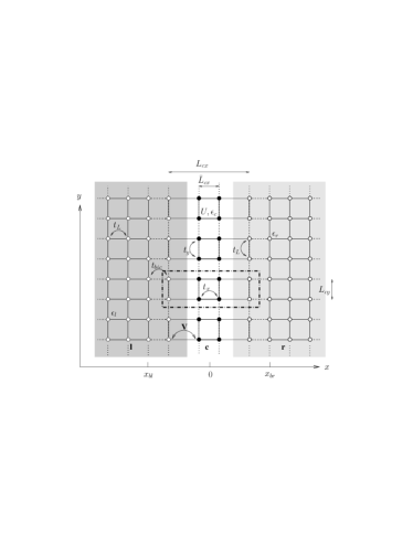
Figure 1: Generic scheme of the model studied here: full (empty) circles indicate correlated (uncorrelated) lattice sites. Correlated sites define the correlated region (c), and are characterized by an on-site Hubbard interaction $U$, an on-site energy $\epsilon_{c}$, and by hopping elements $t_{x}$ and $t_{y}$ in the $x$ and $y$ direction, respectively. The physical leads (l,r), indicated by the two shaded areas, consist of half-infinite planes described by uncorrelated tight-binding models with hopping $t_{L}$, on-site energies $\epsilon_{l}$ and $\epsilon_{r}$, and chemical potentials $\mu_{l}$ and $\mu_{r}$, respectively. The correlated region is connected to the leads via hoppings $V$. The width (number of sites in the $x$ direction) of the correlated region is $\bar{L}_{cx}$. The height of the whole system in the $y$ direction is infinite. In this work, we study two cases, a strongly correlated chain ($\bar{L}_{cx}=1$) and a strongly correlated two-leg ladder ($\bar{L}_{cx}=2$), both perpendicular to the applied bias. In the variational cluster calculation the central region described by the unperturbed Hamiltonian $h$ can differ from the physical one. The latter coincides with the correlated sites (white area in the figure). cen On the other hand, the former consists of disconnected clusters aligned along the $y$ direction, one of them being represented by the dash-dotted rectangle in the figure. The corresponding equilibrium Green’s function is determined by Lanczos exact diagonalization. The size of these clusters is $L_{c}=L_{cx}\times L_{cy}$ ($4\times 2$ in the example). The coordinates of the left and right boundary sites of the central region are indicated by $x_{bl}$ and $x_{br}$, respectively. Accordingly, dashed lines represent hopping processes, which are omitted in the unperturbed (reference) Hamiltonian $h$ and are re-included perturbatively within $\hat{T}$. Full lines indicate hopping terms present in $h$, which are thus treated exactly (see text).

The physical model of interest consists of a “left” and “right” noninteracting lead, as well as a correlated region described by the Hamiltonians $\bar{h}_{l}$, $\bar{h}_{r}$, and $\bar{h}_{c}$, respectively, see Fig. 1. $\bar{h}_{c}$ contains local (Hubbard-type) interactions, as well as arbitrary single-particle terms. For $\tau<\tau_{0}$, the three regions are in equilibrium with three reservoirs at different chemical potentials, $\mu_{l}$, $\mu_{r}$, and $\mu_{c}$ respectively. The correlated region is much smaller in size than the leads, so that the latter act as relaxation baths. At $\tau=\tau_{0}$, the single particle (i. e., hopping) Hamiltonian terms $\hat{V}_{lc}$ and $\hat{V}_{rc}$ are switched on. These connect the left and right reservoir, respectively, with the correlated region. The total time-dependent Hamiltonian is, thus, given by

$$H(\tau)=\bar{h}+\theta(\tau-\tau_{0})\hat{\bar{T}}\;,$$ (1)

where $\bar{h}=\bar{h}_{c}+\bar{h}_{l}+\bar{h}_{r}$, and $\hat{\bar{T}}=\hat{V}_{lc}+\hat{V}_{rc}$. We consider here the fermionic case, although many concepts can be easily extended to bosons. After a time $\Delta\tau$ long enough for relaxation to take place, the system reaches a nonequilibrium steady-state, with a particle current flowing from left to right for $\mu_{l}>\mu_{r}$ and from right to left for $\mu_{l}<\mu_{r}$.

As discussed above, the total $\tau>\tau_{0}$ Hamiltonian $H\equiv H(\tau>\tau_{0})$ is decomposed into an unperturbed part $h$ and a perturbation $\hat{T}$:

$$H=h+\hat{T}\;.$$ (2)

In the simplest CPT approach for a “small” correlated region one can take $h=\bar{h}$, and $\hat{T}=\hat{\bar{T}}$. However, when the correlated region is extended, as in Fig. 1, it has to be further decomposed into smaller clusters that can be solved by exact diagonalization. lea In this case, the intercluster hopping is subtracted from $h$ and must be included in $\hat{T}$. In addition, one can include part of the leads into the clusters (dashed lines in Fig. 1), so that $\hat{V}_{lc}+\hat{V}_{rc}$ are incorporated into $h$, while the leads intercluster hoppings (e.g. $t_{bic}$ in the figure) are included cen in $\hat{T}$. Finally, in the spirit of VCA, arbitrary intracluster terms $\Delta h$ can be added to the unperturbed Hamiltonian and subtracted perturbatively within $\hat{T}$. In other words, calling $h_{cl}$ the Hamiltonian describing the physical cluster partition, and $\hat{T}_{cl}$ the one describing the intercluster hoppings (dashed lines in Fig. 1), we write $h=h_{cl}+\Delta h$, and $\hat{T}=\hat{T}_{cl}-\Delta h$ so that the total Hamiltonian remains unchanged:

$$H=h_{cl}+\hat{T}_{cl}=h+\hat{T}\;.$$ (3)

The arbitrariness in the choice of $\Delta h$ can be exploited to optimize the unperturbed state, as discussed in Ref. Knap et al., 2011 for the equilibrium case. Here, we will adopt a different optimization criterion, see discussion below. Being a single-particle term, $\hat{T}$ is described by its hopping matrix $T$. This matrix has a block structure according to the three regions discussed above and shall be denoted by $T_{lc}$, $T_{rc}$ and $T_{cc}$, respectively.

Nonequilibrium properties, in general, and nonlinear transport in particular can quite generally be determined in the frame of the Keldysh Green’s function approach. Kadanoff and Baym (1962); Schwinger (1961); Keldysh (1965); Haug and Jauho (1998); Rammer and Smith (1986) Here, we adopt the notation of Ref. Rammer and Smith, 1986, for which the $2\times 2$ Keldysh Green’s function matrix is expressed as

$$G({\bf r},{\bf r}^{\prime}|\tau,\tau^{\prime})=\left(\begin{array}[]{ll}G^{R}&G^{K}\\ 0&G^{A}\end{array}\right)\;,$$ (4)

where the retarded ($G^{R}$), advanced ($G^{A}$), and Keldysh ($G^{K}$) Green’s functions depend in general on two lattice sites (${\bf r},{\bf r}^{\prime}$) and two times ($\tau,\tau^{\prime}$). However, both for $\tau<\tau_{0}$ as well as in steady state, time translation invariance holds, so that Green’s functions depend only on the time difference $\tau-\tau^{\prime}$, and we can Fourier transform to frequency space $\omega$.

We use uppercase letters $G$ to denote Green’s functions of the full Hamiltonian $H$, and lowercase $g$ for the ones of the unperturbed Hamiltonian $h$. The advantage of using the Keldysh Green’s function matrix representation is that one can express Dyson’s equation in the same form as in equilibrium. Haug and Jauho (1998); Rammer and Smith (1986) In our case, we can express it in the form

$$G=g+g\ (T+\Delta\Sigma)\ G\;,$$ (5)

where $g=\text{diag}\big{(}g_{ll},\,g_{cc},\,g_{rr}\big{)}$ is block diagonal, and the products have to be considered as matrix multiplications. fre In (5), $\Delta\Sigma=\Sigma-\Sigma_{h}$ is the difference between the (unknown) self-energy $\Sigma$ of the total Hamiltonian $H$, including the coupling to the leads, and the self-energy $\Sigma_{h}$ associated with the unperturbed Hamiltonian $h$.

The CPT approximationSénéchal et al. (2000) precisely amounts to neglecting $\Delta\Sigma$. As pointed out in Ref. Balzer and Potthoff, 2011 this corresponds to neglecting irreducible diagrams containing interactions and one or more $T$ terms. It should, however, be stressed that the self-energy of the isolated clusters is exactly included in $g_{cc}$, which is obtained by Lanczos exact diagonalization.

In this approximation, (5) can be used to obtain an equation for the Green’s function $G_{cc}$ projected onto the central region, which is still a matrix in the lattice sites of the central region and in Keldysh space mno (this is a straightforward generalization of, e.g., the treatment in Ref. Haug and Jauho, 1998):

$$G_{cc} =g_{cc}+g_{cc}\big{(}\ T_{cc}\ G_{cc}+\negthickspace\negthickspace\displaystyle\sum_{\alpha}^{\in\{l,r\}}T_{c\alpha}\ G_{\alpha c}\big{)}$$ (6)

and for the lead-central region Green’s functions:

$$G_{\alpha c} =g_{\alpha\alpha}\ T_{\alpha c}\ G_{cc}\;,\qquad\text{with }\alpha\in\{l,r\}.$$ (7)

It is noteworthy that Eq. (7) is exact and not based on the CPT approximation, as the leads contain non-interacting particles. Insertion of (7) into (6) yields

$$G_{cc} =g_{cc}+g_{cc}\big{(}T_{cc}+\tilde{\Sigma}_{cc}\big{)}\ G_{cc}$$ (8)

with the lead-induced self-energy renormalization

$$\tilde{\Sigma}_{cc} =\displaystyle\sum_{\alpha}^{\in\{l,r\}}T_{c\alpha}\ g_{\alpha\alpha}\ T_{\alpha c}\;.$$ (9)

Here $g_{\alpha\alpha}$ stands for the Green’s function of the isolated lead $\alpha$. One finally obtains a Dyson form for the steady state Green’s function of the coupled system at the central region

$$G_{cc}^{-1}=g_{cc}^{-1}-T_{cc}-\tilde{\Sigma}_{cc}\;.$$ (10)

Different from the usual Dyson equation, $g_{cc}$ is the Green’s function for the isolated clusters, which contains all many-body effects inside the cluster.

For the evaluation of the current from, say, the left lead to the central region cen one needs the $G_{lc}$ Green’s function, which is readily obtained by combining (7) with (10). This leads to the generalized Kadanoff-Baym equation (see e. g. Refs. Haug and Jauho, 1998; Meir and Wingreen, 1992), along with the fact that the central region is finite in $x$ direction and the leads are infinite, one can rewrite the current into a Büttiker-Landauer type of formula

$$j=\int\frac{d\varepsilon}{2\pi} \big{[}f_{F}(\varepsilon-\mu_{r})-f_{F}(\varepsilon-\mu_{l})\big{]}$$

$$\times\operatorname{\mbox{Tr}}\big{[}\;{\sideset{}{{}_{cc}^{R}}{\operatorname{G}}}\;(\varepsilon)\Gamma_{l}(\varepsilon)\;{\sideset{}{{}_{cc}^{A}}{\operatorname{G}}}\;(\varepsilon)\Gamma_{r}(\varepsilon)\big{]}\;.$$ (11)

where $G^{R/A}_{cc}$ is the retarded/advanced part of the Green’s function $G_{cc}$, and the trace, as well as matrix products run over site indices in $c$. $\Gamma_{\alpha}$ describes the inelastic broadening owing to the coupling to lead $\alpha$, which in CPT is given by rea

$$\Gamma_{\alpha} =2\operatorname{\mbox{Im}}\big{\{}T_{c\alpha}g^{A}_{\alpha\alpha}T_{\alpha c}\big{\}}\;,$$

which represents the contribution of lead $\alpha$ to the imaginary part of $\tilde{\Sigma}_{cc}^{A}$. Interestingly, the expression for the current in CPT has the same structure as the Meir-Wingreen formula Meir and Wingreen (1992) for non-interacting particles, which is the basis for nonequilibrium ab-initio-calculations.Fürst et al. (2008) Here, however, the Green’s function contains the many-body interactions of the correlated region. An advantage of this expression is that it yields an explicit connection to the Green function $G^{R/A}_{cc}$ of the scattering region and the influence of the itinerant electrons in the leads. A similar expression can be derived for the one-particle density matrix between two sites with the same $y$ coordinate, which is required for the self-consistency condition discussed below.

As it is well known, all retarded and advanced Green’s functions are evaluated without chemical potentials. The latter enter through the Keldysh Green’s function or rather via the Fermi functions. While the chemical potential of the central region is wiped out in the steady state due to its small size in comparison to the size of the leads, the chemical potentials of the leads explicitly enter the expressions for the current and the density matrix, see Eq. (11). In the case investigated here, the central region is translation invariant in $y$ direction and is split into identical clusters. In the end, as far as the main numerical task is concerned, one has to solve many-body problems for clusters of size $L=L_{cx}\times L_{cy}$, invert matrices of the same size, and sum over wave vectors $q_{y}$ belonging to the Brillouin zone associated with the cluster supercell.

II.2 Self-consistency condition

Equation (10) is the expression for the Green’s function of the central region within the CPT approximation. As discussed above, one would like to optimize the initial state in some appropriate way by suitably adjusting the parameters $\Delta h$ of the unperturbed Hamiltonian $h$. The inclusion of additional terms $\Delta h$ adds flexibility to the self-energy $\Sigma_{h}$ which is included within this approximation. Obviously, it makes no difference in the case of non-interacting particles as the selfenergy vanishes exactly, independently of $\Delta h$. This freedom can be exploited in order to improve the approximation systematically. A similar discussion on this issue has been given in Refs. Dahnken et al., 2004; Knap et al., 2011), and is at the basis of the VCA idea Potthoff (2003a).

As discussed above, we need a variational condition associated with a “minimization” of the difference between unperturbed and perturbed state. In (cluster)-DMFT one requires the cluster projected Green’s function to be equal to the unperturbed one

$$g_{cc}={\cal P}(G_{cc})\;,$$ (12)

where ${\cal P}$ projects the Green’s function onto the cluster, i. e., it sets all its intercluster matrix elements to zero. coi Since here we have a finite number of variational parameters ${\bf p}$ that can be adjusted, we cannot satisfy (12). We, thus, propose a “weaker” condition, namely that the expectation values of operators coupled to the variational parameters contained in $\Delta h$ (i. e., $d\Delta h/d{\bf p}$) be equal in the unperturbed and in the perturbed state. More specifically, we impose the condition

$$\int\frac{d\omega}{2\pi}\operatorname{\mbox{tr}}\hat{\tau}_{1}\frac{\partial\left(g_{0cc}\right)^{-1}}{\partial{\bf p}}\left(g_{cc}-G_{cc}\right)=0\;,$$ (13)

where $\hat{\tau}_{1}$ is a Pauli matrix in Keldysh space, tau and $g_{0cc}$ is the Green’s function associated with the noninteracting part of $h$. It is interesting to note (see appendix  A) that by including into $\Delta h$ a coupling to an infinite number of bath sites, the present method, with the self-consistence condition (13) whereby ${\bf p}$ are the bath parameters (hopping and on-site energies), becomes equivalent to nonequilibrium cluster DMFT. Generalization of the SFA condition to nonequilibrium should be, in principle, obtained by replacing $g_{0cc}$ with $\Sigma_{h}$ in (13).

A second systematic improvement of this nonequilibrium VCA approach consists in increasing the cluster size $L_{c}$. This can be done in two ways: (i) by extending the boundaries of the central region in $y$ direction and thus treating more correlated sites exactly cen and (ii) by extending the boundaries in $x$ direction to include an increasing number of uncorrelated lattice sites, i. e., taking $L_{cx}>\bar{L}_{cx}$, cf. Fig. 1. This amounts to taking into account to some degree the $V$-induced renormalization of the self-energy.

III Model

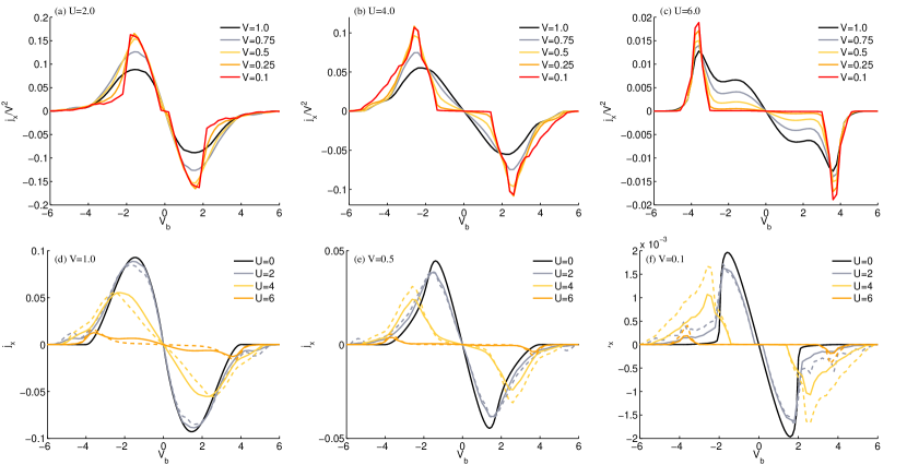
Figure 2: (Color online) Steady-state current density $j_{x}$ versus bias voltage $V_{b}$ for a correlated two-leg ladder ($\bar{L}_{cx}=2$). First row shows $j_{x}$ normalized by $V^{2}$ as function of $V_{b}$ evaluated for different values of $V$ and of the interaction (a) $U=2.0$, (b) $U=4.0$, and (c) $U=6.0$. Second row shows the $U$ dependence of the current for different values of the hopping $V=V_{lc}=V_{rc}$ from the leads to the correlated region (d) $V=1.0$, (e) $V=0.5$, and (f) $V=0.1$. Solid (dashed) lines represent results for the current between the left lead and the central region (between two in $x$ direction adjacent sites inside the central region), i. e., evaluated with $G_{lc}^{K}$ ($G_{cc}^{K}$), see text for details. Results are obtained by using a reference Hamiltonian $h$ consisting of disconnected clusters of size $L_{c}=L_{cx}\times L_{cy}=2\times 6$.

Next, we present an application of the nonequilibrium VCA method described in Sec. II. Specifically, we study nonlinear transport properties across an extended correlated region (denoted as $c$ in Fig.1), which we take to be a Hubbard chain ($\bar{L}_{cx}=1$) or a Hubbard ladder ($\bar{L}_{cx}=2$) with nearest-neighbor hoppings $t_{x}$ and $t_{y}$, on-site interaction $U$, on-site energy $\epsilon_{c}$, and chemical potential $\mu_{c}$

$$\bar{h}_{c}=\sum_{\langle i,j\rangle,\,\sigma}t_{ij}c_{i\sigma}^{\dagger}c_{j\sigma}^{\phantom{\dagger}}+U\sum_{i}\hat{n}_{i\uparrow}\hat{n}_{i\downarrow}+(\epsilon_{c}-\mu_{c})\sum_{i,\sigma}\hat{n}_{i\sigma}\;,$$

in usual notation, and where $t_{ij}=t_{x}$ ($t_{ij}=t_{y}$) for $i$ and $j$ being nearest neighbors in $x$ direction ($y$ direction). The leads (shaded regions in Fig. 1) are described by two-dimensional semi-infinite tight-binding models with nearest-neighbor hopping $t_{L}$, on-site energies $\epsilon_{l}$ and $\epsilon_{r}$, and chemical potentials $\mu_{l}$ and $\mu_{r}$ for the left and right lead, respectively. We apply a bias voltage $V_{b}$ to the leads by setting $\mu_{r}=\epsilon_{r}=V_{b}/2$ and restrict to the particle-hole symmetric case where $\epsilon_{c}=-U/2$, $\mu_{c}=0$, $\epsilon_{r}=-\epsilon_{l}$, and $\mu_{l}=-\mu_{r}$. For simplicity, we neglect the long-range part of the Coulomb interaction. Under some conditions, this can be absorbed within the single-particle parameters of the Hamiltonian, in a mean-field sense. Haug and Jauho (1998)

As discussed above, the unperturbed Hamiltonian $h$ does not necessarily coincide with the physical partition into leads and correlated region. $h$ is obtained by tiling the total system into small clusters as illustrated in Fig. 1, as well as by adding an intracluster variational term $\Delta h$.

In the present work $\Delta h$ describes a correction $\Delta t_{x}$ to the intra-ladder hopping. Further options could include, for instance, a site-dependent change in the on-site energy $\Delta\epsilon_{c}(x)$. Particle-hole symmetry can be preserved by constraining this change to be antisymmetric: $\Delta\epsilon_{c}(x)=-\Delta\epsilon_{c}(-x)$. In this paper, whose goal is to carry out a first test of the method, we restrict, for simplicity, to a single variational parameter. The choice of $\Delta t_{x}$ as a variational parameter is motivated by the fact that this term is important for the current flowing in $x$ direction. According to the prescription discussed above, we require the expectation value of the one-particle density matrix for nearest-neighbor indices in $x$ direction to be the same for the unperturbed $h$ and for the full $H$, i.e. evaluated with $g_{cc}$ and with $G_{cc}$.

One comment about the chemical potential. In principle, when including some of the sites of the leads in $h$, i. e., when $L_{cx}>\bar{L}_{cx}$, then these additional sites have a chemical potential $\mu_{c}$ which differs from the one they would have if $L_{cx}=\bar{L}_{cx}$ (i. e., $\mu_{l}$ or $\mu_{r}$). However, the chemical potential, of these sites does not affect the steady state, as their volume-to-surface ratio is finite. Of course, their on-site energies ($\epsilon_{r}$ and $\epsilon_{l}$) are important.

Due to translation invariance by a cluster length $L_{cy}$ in the $y$ direction, it is convenient, as in usual VCA, to carry out a Fourier transformation in $y$ direction, with associated momenta $q_{y}$. The Green’s functions $g_{cc}$ and $G_{cc}$, as well as $T$ become now functions of two momenta $q_{y}+Q_{y}$ and $q_{y}+Q_{y}^{\prime}$, where $Q_{y}$ and $Q_{y}^{\prime}$ are reciprocal superlattice vectors of which there are only $L_{cy}$ inequivalent ones. In order to evaluate the nonequilibrium steady state, one only needs the equilibrium Green’s function $g(x_{b\alpha}|q_{y}|z)$ of the isolated leads at the contact edge to the central region, with $x$ coordinate equal to $x_{b\alpha}$ ($\alpha\in\{l,\,r\}$), and Fourier transformed in the $y$ directions, where $q_{y}$ is the corresponding momentum and $z$ the complex frequency. For a semiinfinite nearest-neighbor tight-binding plane with hopping $t_{L}$, and on-site energy $\epsilon_{\alpha}$, this can be expressed as

$$g(x_{b\alpha}|q_{y}|z)=g_{c,loc}(z-2t_{L}\cos q_{y}-\epsilon_{\alpha})\;,$$ (14)

where $g_{c,loc}(z)$ is the local Green’s function of a tight binding chain with open boundary conditions and with zero on-site energy. The latter can be determined analytically along the lines discussed in Ref. Economou, 2006.

The model studied here, is motivated by the interest in transport across semiconductor heterostructures (see, e.g. Pérez-Merchancano et al., 2008; Ertler et al., 2010a, b; Chioncel et al., 2011). However, it is well known that in this case charging effects are important, also near the boundaries between the leads and the central region. Here, scattering effects produce charge density waves, which, when taking into account the long-range part of the Coulomb interaction, even in mean-field, produce a modification of the single-particle potential. In order to treat realistic structures, these effects should be included at the Hartree-Fock level at least. All these generalizations can be straightforwardly treated with the presented variational cluster method, however, in this work we focus on a first proof of concept study and application containing the essential ingredients for the investigation of the nonequilibrium steady state of strongly correlated many-body systems.

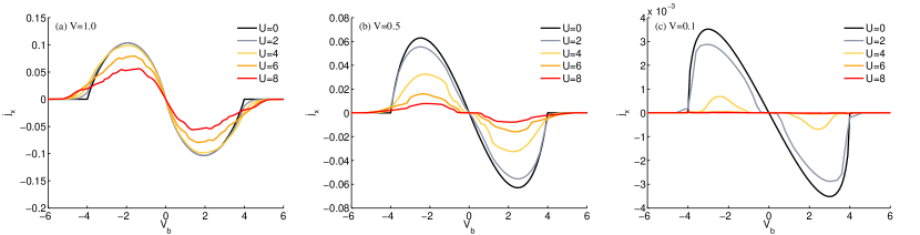
Figure 3: (Color online) Steady-state current density $j_{x}$ as in Fig. 2 but for the correlated chain ($\bar{L}_{cx}=1$). The current density is evaluated for different values of the lead to correlated region hopping (a) $V=1.0$, (b) $V=0.5$, and (c) $V=0.1$, and of the interaction $U$, see legend. Results are obtained for reference clusters of size $L_{c}=L_{cx}\times L_{cy}=3\times 4$.

IV Results

We have evaluated the steady-state current density $j_{x}$ of the models discussed in Sec. III as a function of the bias $V_{b}\equiv\epsilon_{r}-\epsilon_{l}$ between the leads at zero temperature. Simultaneously the chemical potential is adjusted to the on-site energy $\mu_{\alpha}=\epsilon_{\alpha}$, which corresponds to a rigid shift of the density of states in both leads in opposite directions.

In Fig. 2 we display results for the two-leg ladder ($\bar{L}_{cx}=2$), for different values of the interaction strength $U=\{0,\,2,\,4,\,6\}$ and lead-to-system hopping $V=\{1.0,\,0.75,\,0.5,\,0.25,\,0.1\}$. We use $\hbar=1$ and $t_{L}=1$ which sets the unity of energy. Moreover, we take the lattice constant $a=1$. The hopping is uniform in the whole system, meaning that $t_{x},\,t_{y}$ in the correlated region and $t_{L}$ of the leads are equal. The on-site energy of the correlated region is $\epsilon_{c}=-U/2$ corresponding to half-filling, whereas the on-site energy of the left (right) lead is equal to its chemical potential $\mu_{l}$ ($\mu_{r}$). The unperturbed hamiltonian $h$ describes the central region decomposed into clusters of size $L_{c}=2\times 6$. The corresponding Green’s function $g_{cc}$ is determined exactly by Lanczos diagonalization. All results are determined self-consistently using $\Delta t_{x}$ as variational parameter, see Sec. III.

Using the Meir-Wingreen expression, Eq. (11), the general trend of the results for the steady-state current $j_{x}$ can be discussed conveniently. At zero temperature there are only contributions to the current for $\min(\mu_{l},\mu_{r})<\omega<\max(\mu_{l},\mu_{r})$ due to the difference of the Fermi distribution functions. In particular this leads as expected to zero current for zero bias voltage $V_{b}$. With increasing bias voltage $V_{b}$ the modulus of $j_{x}$ initially increases. For large values of $V_{b}$ it decreases again, as the overlap of the local density of states of the two leads enters the expression, which is zero if $V_{b}$ is greater than the band width of the leads. Hence the local density of states of the leads along with the Fermi function act as a filter that averages the electronic excitations of the central region within a certain energy window.

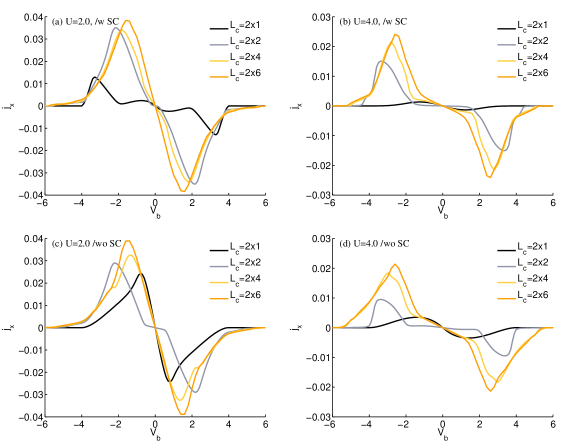
Figure 4: (Color online) Convergence of the steady-state current density $j_{x}$ with reference cluster size $L_{c}=L_{cx}\times L_{cy}$ for the correlated two-leg ladder with $V=0.5$. Results in (a), (b) are obtained by a variational adjustment of the intra-cluster hopping $t_{x}$ as discussed in the text, while those of (c), (d) are obtained without modification of $t_{x}$. The values for the Hubbard interaction are $U=2$ in [(a), (c)] and $U=4$ in [(b), (d)].

In the system we are studying, the leads are modeled by semi-infinite tight binding planes. Alternatively, instead of using (14) one could simply put a model Green’s function “by hand,” as for example one which describes a Lorentzian shaped density of states. Such an unbound density of states generally leads to a finite value of the current for arbitrary bias.

The leads have a further effect on the result as they provide an inelastic broadening of the energy spectrum of the central region entering $\Sigma^{\text{eff}}$, see Eq. (10), which smears out details of the excitation spectrum. As far as the lead-correlated region coupling $V$ is concerned, there are two competing effects: on the one hand, the current increases with increasing $V$ due to the stronger coupling between the correlated region and the leads. On the other hand, details of the electronic excitations are smeared out with increasing $V$ leading to a reduced resolution. Therefore, in order to detect the effects of strong correlations, particularly the gap, a small value for $V$ is required.

The details of the $V$ dependence of $j_{x}$ for small $V$ can be deduced from (11). Here, the expression for the current has a prefactor proportional to $V^{4}$ (at least in the $L_{cx}=\bar{L}_{cx}$ case), due to the two $\Gamma$ terms. On the other hand, for a gapless system, there is a $V^{2}$ term in the denominator of $|G_{cc}^{R}|^{2}$. For a gapped system, this is cut off by the energy gap $E_{g}$, so that in this case $j_{x}\sim V^{4}/E_{g}^{2}$, while $j_{x}\sim V^{2}$ for a gapless spectrum. These aspects are clearly observable in Fig. 2 (a)–(c), which shows the scaled current density $j_{x}/V^{2}$ for fixed interaction strength $U$ but varying $V$. The envelope has a rotated S-like structrue due to the combined effects of the lead density of states and of the Fermi functions.

Next we will analyze a bit more in detail the effects of the Hubbard interaction. Increasing the interaction strength $U$ in the correlated region leads to a suppression of the current and the opening of a gap, which is best oberserved in (f). For $U=4$ the maximum of the current density is roughly reduced by a factor of two as compared to the noninteracting case, whereas for $U=6$ the current is almost one order of magnitude smaller as compared to the noninteracting system, see Fig. 2 (d)–(f).

Finally, we want to address the the difference between the solid lines and dashed lines in the the panels (d)–(f) of Fig. 2, which represent the current density evaluated on a bond connecting the leads to the central region, or on a bond within the two-leg ladder. Due to the stationary condition, the two results should coincide. However, our calculations shows a slight discrepancy between them, which is due to the fact that the method is not completely conserving and, thus, the continuity equation is not completely fulfilled. However, from our results we see that the deviation from the continuity equation is quite small. We expect this discrepancy to be reduced upon improving the optimization with the introduction of additional variational parameters.

In Fig. 3 we show the steady-state current density $j_{x}$ across the correlated chain ($\bar{L}_{cx}=1$) as a function of the bias voltage. The parameters are the same as in the case of the two-leg ladder, however, the central region is decomposed into clusters of size $L_{c}=3\times 4$, where also sites of the leads are taken into account to improve the results. The half-filled Hubbard chain is gapped as well. As for the two-leg ladder, the gap behavior can be better seen in the current-voltage characteristics for smaller values of $V$, in our case for $V=0.1$. In contrast, for strong coupling $V=1.0$, (a), no gap behavior can be seen in the current due to the strong hybridization with the leads.

For strong values of the coupling $V$ between leads and correlated region ($V=1.0$), (a), the current is significant for all values of the interaction $U$. However, with decreasing $V$, (b)–(c), the current is strongly suppressed for large interaction $U$. Importantly, for the correlated chain the continuity equation is always strictly fulfilled. In other words, there is no difference between $j_{x}$ evaluated on a intercluster bond between the leads and the cluster, or on an intracluster bond. This is due to the absence of vertex corrections at the uncorrelated sites.

Next, we study the convergence of our results with the size of the cluster, as well as the effect of the self-consistency condition for the two-leg ladder and $V=0.5$. Results are depicted in Fig. 4 for two different values of the Hubbard interaction, namely $U=2$ [(a), (c)] and $U=4$ [(b), (d)]. We do not plot results of the convergence analysis for $U=6$, since for this large $U$ the current is already rather small, as can be seen in Fig. 2 (d)–(f). Results in (a) and (b), first row, are obtained by adjusting $\Delta t_{x}$ self-consistently, as described in Sec. III, whereas (c) and (d), second row, shows results without self-consistency, i. e., with $\Delta t_{x}=0$. Results show that the self-consistency procedure improves the results, as the convergence for $j_{x}$ is faster with increasing cluster size as compared to the case without self-consistency. Generally, we observe pronounced finite size effects for very small clusters up to $2\times 4$, and convergence seems to be reached for the $2\times 6$ cluster.

We now repeat the same analysis for the correlated chain. The corresponding current densities for the parameters $U=2$ and $V=0.5$ are shown in Fig. 5 for different cluster sizes.

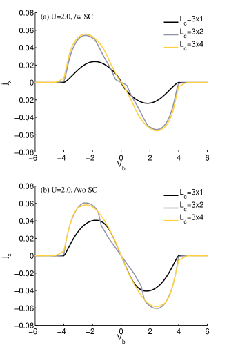
Figure 5: (Color online) Convergence of the steady-state current density $j_{x}$ with reference cluster size $L_{c}=L_{cx}\times L_{cy}$ for the correlated chain. Results in (a) fulfill the self-consistency condition (13), whereas results in (b) do not. The parameters are $U=2$ and $V=0.5$.

Results shown in (a) are with self-consistency procedure (13), whereas the results shown in (b) are without. In the present case, where we consider transport across a strongly correlated chain, convergence is achieved very quickly with increasing cluster size. Therefore, there is no sensible difference between results obtained with or without self-consistency, apart for the pathological case $L_{c}=3\times 1$ (see below).

Results obtained for the two-leg ladder and for the chain show that cluster geometries with $L_{cy}=1$ provide results far from convergence, even with self-consistency. For the chain this is probably due to the degeneracy of the cluster ground state. For the ladder, it seems that using as starting point the $2\times 1$ dimer exaggerates the gap. But besides these data obtained from admittedly very small clusters, results converge quickly as a function of cluster sizes, especially when the hopping in $x$ direction is used as a variational parameter.

V Conclusions

In this paper we have presented a novel approach to treat strongly correlated systems in the nonequilibrium steady state. The idea is based on the variational cluster approach extended to the Keldysh formalism. For the present approach the expression for the current resembles the corresponding Meir-Wingreen formulas. As in the original Meir-Wingreen approach, which is also the basis for nonequilibrium density-functional based calculations, we directly address the steady state behavior of a device coupled to infinite leads. The latter is necessary for the system to reach a well-defined steady state.

The present nonequilibrium extension is in a similar spirit to the equilibrium self-energy functional approach, in which one “adds” single-particle terms to the cluster Hamiltonian which is then solved exactly, and “subtract” them perturbatively. Dahnken et al. (2004); Knap et al. (2011) The values of the parameters are determined by an appropiate requirement which in the end amounts to optimizing the unperturbed state with respect to the perturbed one.

There is a certain freedom in choosing the most appropriate self-consistency criterion. Here we have required the operators associated with the variational parameters to have the same expectation values in the unperturbed and in perturbed state. Certainly, an interesting alternative would be to generalize the variational criterion provided by the self-energy functional approach Potthoff (2003a) to the nonequilibrium case. This will be obtained by a suitable generalization of the Euler equation (Eq. (7) of Ref. Potthoff, 2003a) to the Keldysh contour, i. e., by replacing $g_{0cc}$ with the self-energy $\Sigma_{h}$ in (13) Work along these lines is in progress.

The advantage of the present variational condition (13) is that it is computationally less demanding, as one just needs to evaluate cluster single-particle Green’s functions. Which one of the two conditions gives more accurate results cannot be stated a priori and should be explicitly checked.

In any case, both methods, the self-energy functional approach and the present one, become equivalent to (cluster) dynamical mean-field theory in the case in which an infinite number of variational parameters is suitably taken (see Appendix A).

In general, we expect results to improve when more variational parameters are taken into account. In particular, when evaluating the current across the central region, it would be useful if a current was already flowing in the cluster. This can be achieved by adding a complex variational hopping between the end points of the cluster, and of course remove it perturbatively. The corresponding variational condition would contain the interesting requirement that the current flow in this modified cluster be the same as in steady state.

The model studied here, is motivated by the interest in transport across semiconductor heterostructures (see, e.g. Pérez-Merchancano et al., 2008; Ertler et al., 2010a, b; Chioncel et al., 2011). However, it is well known that in this case charging effects are important, also near the boundaries between the leads and the correlated region. Here, scattering effects produce charge density waves, which, when taking into account the long-range part of the Coulomb interaction, even in mean-field, produce a modification of the single-particle potential. In order to treat realistic structures, these effects should be included at the Hartree-Fock level at least. All these generalizations can be straightforwardly treated with the presented variational cluster method, however, in this work we focus on a first proof of concept study and application containing the essential ingredients for the investigation of the nonequilibrium steady state of strongly correlated many-body systems.

Appendix A Connection to (cluster) Dynamical Mean-Field Theory

Here, we show that the self-consistent condition (13) provides a bridge to (cluster) DMFT, when an increasing number of noninteracting bath sites with appropriate parameters and occupations is included in the cluster Hamiltonian. Notice that these are “auxiliary” baths and are not related to the leads. Concretely, this is achieved by introducing into the variational Hamiltonian $\Delta h$ a coupling of the central region with a set of uncorrelated bath sites with appropriate energies, hybridizations $v^{\pm}_{n}$, and occupations (see below). The hybridizations $v^{\pm}_{n}$ and the energies are therefore “included” in $h$, but “subtracted perturbatively,” from the target Hamiltonian $H$. Their parameters are determined variationally via (13).

Now, since $g_{0cc}$ is cluster-local, a solution to (13) is obviously given by (12). However, this solution can generally not be obtained with a finite number of parameters. As in usual equilibrium (cluster) DMFT, Georges et al. (1996) (12) can thus be solved via an iterative procedure defined by

$$g_{0cc,new}^{-1} =\left({\cal P}(G_{cc})\right)^{-1}+\Sigma_{h}$$

$$\Sigma_{h} =g_{0cc,old}^{-1}-g_{cc}^{-1}\;.$$ (15)

It is, thus, sufficient to show that an arbitrary $g_{0cc,new}$ can be obtained by coupling the cluster to a noninteracting bath with suitably chosen bath parameters. For the retarded and advanced Green’s functions, the procedure is the same as in equilibrium. The Keldysh part is slightly more complicated. In order to show that an aribrary $g_{0cc,new}$ can be realized, one introduces the hybridization function

$$\Delta(\omega)=\left(\begin{array}[]{cc}\Delta^{R}(\omega)&\Delta^{K}(\omega)\\ 0&\Delta^{A}(\omega)\end{array}\right)\;,$$ (16)

where the $\Delta^{R}$, $\Delta^{A}$, and $\Delta^{K}$ are matrices in the cluster sites. Similarly to equilibrium DMFT $g_{0cc,new}$ is expressed as

$$g_{0cc,new}^{-1}=g_{0cc,0}^{-1}-\Delta(\omega)\;.$$ (17)

Here, $g_{0cc,0}^{-1}$ is the “bare” noninteracting cluster Green’s function, i. e., the one with neither baths nor variational parameters.

An arbitrary (steady-state) $\Delta(\omega)$ can be produced by coupling the central region to an appropriate bath in the following way. The retarded (and advanced) part are obtained as in equilibrium DMFT Georges et al. (1996) by coupling to a bath with spectral function imr $A_{bath}(\omega)$ given by

$$\ A_{bath}(\omega)=-\frac{1}{\pi}\operatorname{\mbox{Im}}\Delta^{R}(\omega)\;,$$ (18)

($\text{Re}\,\Delta^{R}$ is fixed by Kramers-Kronig relations). On the other hand, the Keldysh part is generated by splitting the bath defined by (18) into two baths, a full ($\mu=\infty$) and an empty ($\mu=-\infty$) one, respectively. Their spectral functions are denoted by $A_{bath}^{+}(\omega)$ and $A_{bath}^{-}(\omega)$, respectively, and should obviously fullfill the condition

$$A_{bath}(\omega)=A_{bath}^{+}+A_{bath}^{-}\;.$$ (19)

Since the Fermi functions of the two baths are $1$ and $0$, respectively, the Keldysh part $\Delta^{K}(\omega)$ is given by ($\Delta^{K}$ is anti-hermitian)

$$\Delta^{K}(\omega)=-2i\pi\ B_{bath}(\omega)\equiv-2i\pi\ \left(A_{bath}^{-}(\omega)-A_{bath}^{+}(\omega)\right)\;.$$ (20)

This fixes the two spectral functions to be

$$A^{\mp}_{bath}(\omega)=\frac{A_{bath}(\omega)\pm B_{bath}(\omega)}{2}\;.$$ (21)

As usual, the two baths spectral functions $A_{bath,\pm}(\omega)$ are realized by coupling the central region with a set of noninteracting sites with energies $\epsilon^{\pm}_{n}$ and hybridizations imr $v^{\pm}_{n}$, fixed by

$$A_{bath}^{\pm}(\omega)=\sum_{n}v^{\pm}_{n}v^{\pm{\dagger}}_{n}\delta(\omega-\epsilon^{\pm}_{n})\;.$$ (22)

References

- Jaksch et al. (1998) D. Jaksch, C. Bruder, J. I. Cirac, C. W. Gardiner, and P. Zoller, Phys. Rev. Lett. 81, 3108 (1998).
- Greiner et al. (2002) M. Greiner, O. Mandel, T. Esslinger, T. W. Hänsch, and I. Bloch, Nature (London) 415, 39 (2002).
- Bloch et al. (2008) I. Bloch, J. Dalibard, and W. Zwerger, Rev. Mod. Phys. 80, 885 (2008).
- Hartmann et al. (2008) M. Hartmann, F. G. Brandão, and M. B. Plenio, Laser & Photonics Rev. 2, 527 (2008).
- Tomadin and Fazio (2010) A. Tomadin and R. Fazio, J. Opt. Soc. Am. B 27, A130 (2010).
- Park et al. (2000) H. Park, J. Park, A. K. L. Lim, E. H. Anderson, A. P. Alivisatos, and P. L. McEuen, Nature 407, 57 (2000).
- Paaske and Flensberg (2005) J. Paaske and K. Flensberg, Phys. Rev. Lett. 94, 176801 (2005).
- Zutic et al. (2004) I. Zutic, J. Fabian, and S. D. Sarma, Rev. Mod. Phys. 76, 323 (2004).
- Fabian et al. (2007) J. Fabian, A. Matos-Abiague, C. Ertler, P. Stano, and I. Zutic, Acta Physica Slovaca 57, 565 (2007).
- Slobodskyy et al. (2003) A. Slobodskyy, C. Gould, T. Slobodskyy, C. R. Becker, G. Schmidt, and L. W. Molenkamp, Phys. Rev. Lett. 90, 246601 (2003).
- Bonilla and Grahn (2005) L. L. Bonilla and H. T. Grahn, Rep. Prog. Phys. 68, 577 (2005).
- Jungwirth et al. (2006) T. Jungwirth, J. Sinova, J. Masek, J. Kucera, and A. H. MacDonald, Rev. Mod. Phys. 78, 809 (2006).
- Ertler et al. (2010a) C. Ertler, W. Pötz, and J. Fabian, Appl. Phys. Lett. 97, 042104 (2010a).
- Ertler et al. (2010b) C. Ertler, P. Senekowitsch, J. Fabian, and W. Pötz, in Computational Electronics (IWCE), 2010 14th International Workshop on (2010b), pp. 1–4.
- Sokolowski-Tinten et al. (2003) K. Sokolowski-Tinten, C. Blome, J. Blums, A. Cavalleri, C. Dietrich, A. Tarasevitch, I. Uschmann, E. Forster, M. Kammler, M. Horn-von Hoegen, et al., Nature 422, 287 (2003).
- Haug and Jauho (1998) H. Haug and A.-P. Jauho, Quantum Kinetics in Transport and Optics of Semiconductors (Springer, Heidelberg, 1998).
- Rammer and Smith (1986) J. Rammer and H. Smith, Rev. Mod. Phys. 58, 323 (1986).
- Meir and Wingreen (1992) Y. Meir and N. S. Wingreen, Phys. Rev. Lett. 68, 2512 (1992).
- Meir et al. (1993) Y. Meir, N. S. Wingreen, and P. A. Lee, Phys. Rev. Lett. 70, 2601 (1993).
- Ryndyk et al. (2009) D. A. Ryndyk, R. Gutierrez, B. Song, and G. Cuniberti, in Energy Transfer Dynamics in Biomaterial Systems, edited by A. W. Castleman, J. P. Toennies, K. Yamanouchi, W. Zinth, I. Burghardt, V. May, D. A. Micha, and E. R. Bittner (Springer Berlin Heidelberg, 2009), vol. 93 of Springer Series in Chemical Physics, pp. 213–335.
- Schoeller, H. (2009) Schoeller, H., Eur. Phys. J. Special Topics 168, 179 (2009).
- Diehl et al. (2008) S. Diehl, A. Micheli, A. Kantian, B. Kraus, H. P. Büchler, and P. Zoller, Nat. Phys. 4, 878 (2008).
- Kraus et al. (2008) B. Kraus, H. P. Büchler, S. Diehl, A. Kantian, A. Micheli, and P. Zoller, Phys. Rev. A 78, 042307 (2008).
- Diehl et al. (2010) S. Diehl, A. Tomadin, A. Micheli, R. Fazio, and P. Zoller, Phys. Rev. Lett. 105, 015702 (2010).
- Pichler et al. (2010) H. Pichler, A. J. Daley, and P. Zoller, Phys. Rev. A 82, 063605 (2010).
- Tomadin et al. (2011) A. Tomadin, S. Diehl, and P. Zoller, Phys. Rev. A 83, 013611 (2011).
- Barmettler and Kollath (2010) P. Barmettler and C. Kollath, arXiv:1012.0422 (2010).
- Dalla Torre et al. (2010) E. G. Dalla Torre, E. Demler, T. Giamarchi, and E. Altman, Nat. Phys. 6, 806 (2010).
- White and Feiguin (2004) S. R. White and A. E. Feiguin, Phys. Rev. Lett. 93, 076401 (2004).
- Daley et al. (2004) A. J. Daley, C. Kollath, U. Schollwöck, and G. Vidal, J. Stat. Mech. 2004, P04005 (2004).
- Prosen and Žnidarič (2009) T. Prosen and M. Žnidarič, J. Stat. Mech. 2009, P02035 (2009).
- Benenti et al. (2009) G. Benenti, G. Casati, T. Prosen, D. Rossini, and M. Žnidarič, Phys. Rev. B 80, 035110 (2009).
- Perez-Garcia et al. (2007) D. Perez-Garcia, F. Verstraete, M. M. Wolf, and J. I. Cirac, Quant. Inf. Comp. 7, 401 (2007).
- Werner et al. (2009) P. Werner, T. Oka, and A. J. Millis, Phys. Rev. B 79, 035320 (2009).
- Anders and Schiller (2006) F. B. Anders and A. Schiller, Phys. Rev. B 74, 245113 (2006).
- Jakobs et al. (2007) S. G. Jakobs, V. Meden, and H. Schoeller, Phys. Rev. Lett. 99, 150603 (2007).
- Joura et al. (2008) A. V. Joura, J. K. Freericks, and T. Pruschke, Phys. Rev. Lett. 101, 196401 (2008).
- Eckstein et al. (2009) M. Eckstein, M. Kollar, and P. Werner, Phys. Rev. Lett. 103, 056403 (2009).
- Aron et al. (2011) C. Aron, G. Kotliar, and C. Weber (2011), arXiv:1105.5387.
- Freericks et al. (2006) J. K. Freericks, V. M. Turkowski, and V. Zlatić, Phys. Rev. Lett. 97, 266408 (2006).
- Mehta and Andrei (2006) P. Mehta and N. Andrei, Phys. Rev. Lett. 96, 216802 (2006).
- Gritsev et al. (2010) V. Gritsev, T. Rostunov, and E. Demler, J. Stat. Mech. 2010, P05012 (2010).
- Jung et al. (2010) C. Jung, A. Lieder, S. Brener, H. Hafermann, B. Baxevanis, A. Chudnovskiy, A. N. Rubtsov, M. I. Katsnelson, and A. I. Lichtenstein, arXiv:1011.3264 (2010).
- Balzer and Potthoff (2011) M. Balzer and M. Potthoff, Phys. Rev. B 83, 195132 (2011).
- Myöhänen et al. (2009) P. Myöhänen, A. Stan, G. Stefanucci, and R. van Leeuwen, Phys. Rev. B 80, 115107 (2009).
- Brandbyge et al. (2002) M. Brandbyge, J.-L. Mozos, P. Ordejón, J. Taylor, and K. Stokbro, Phys. Rev. B 65, 165401 (2002).
- Fürst et al. (2008) J. A. Fürst, M. Brandbyge, A.-P. Jauho, and K. Stokbro, Phys. Rev. B 78, 195405 (2008).
- Markussen et al. (2009) T. Markussen, A.-P. Jauho, and M. Brandbyge, Phys. Rev. B 79, 035415 (2009).
- Dahnken et al. (2004) C. Dahnken, M. Aichhorn, W. Hanke, E. Arrigoni, and M. Potthoff, Phys. Rev. B 70, 245110 (2004).
- Knap et al. (2011) M. Knap, E. Arrigoni, and W. von der Linden, Phys. Rev. B 83, 134507 (2011).
- Metzner and Vollhardt (1989) W. Metzner and D. Vollhardt, Phys. Rev. Lett. 62, 324 (1989).
- Georges et al. (1996) A. Georges, G. Kotliar, W. Krauth, and M. J. Rozenberg, Rev. Mod. Phys. 68, 13 (1996).
- Kotliar et al. (2001) G. Kotliar, S. Y. Savrasov, G. Pálsson, and G. Biroli, Phys. Rev. Lett. 87, 186401 (2001).
- Potthoff (2003a) M. Potthoff, Eur. Phys. J. B 32, 429 (2003a).
- Potthoff (2003b) M. Potthoff, Eur. Phys. J. B 36, 335 (2003b).
- Nevidomskyy et al. (2008) A. H. Nevidomskyy, D. Sénéchal, and A. M. S. Tremblay, Phys. Rev. B 77, 075105 (2008).
- (57) To avoid confusion, we denote as “correlated region” the “physical” one containing interacting sites, bounded by the hoppings . On the other hand, the “central region” is the one containing the clusters, and is bounded by . (See Fig. 1).
- (58) Obviously, the uncorrelated leads can be solved exactly without being partitioned into clusters.
- Kadanoff and Baym (1962) L. P. Kadanoff and G. Baym, Quantum statistical mechanics: Green’s function methods in equilibrium and nonequilibrium problems (Addison-Wesley, Redwood City, Calif., 1962).
- Schwinger (1961) J. Schwinger, J. Math. Phys. 2, 407 (1961).
- Keldysh (1965) L. V. Keldysh, Sov. Phys. JETP 20, 1018 (1965).
- (62) In the time representation (4) they also include convolutions over internal times. However, since we are considering the steady state, Green’s functions become diagonal in the frequency representation.
- Sénéchal et al. (2000) D. Sénéchal, D. Perez, and M. Pioro-Ladriére, Phys. Rev. Lett. 84, 522 (2000).
- (64) Here, we use a notation to express projection of objects such as , , etc., which are matrices in lattice indices and in Keldysh space, onto one of the three regions , , or . More specifically, let be such a matrix, then refers to a sub-matrix of in which the left (right) index is restricted to region (), with , or .
- (65) For simplicity, we consider all hoppings to be real.
- (66) Notice that when the central region coincides with the cluster, . In this case the solution of (13) is trivially obtained by taking the leads as auxiliary baths.
- (67) The in (13) is due to our choice of convention (4) for the Keldysh matrix. If one uses the form containing the time- and anti-time-ordered Green’s functions in the diagonal, and the greater and lesser in the off-diagonal elements, no is present in the trace.
- Economou (2006) E. N. Economou, Green’s Functions in Quantum Physics (Springer, Heidelberg, 2006).
- Pérez-Merchancano et al. (2008) S. Pérez-Merchancano, H. P. Gutiérrez, and G. E. Marques, Microelectronics Journal 39, 1339 (2008), Papers CLACSA XIII, Colombia 2007.
- Chioncel et al. (2011) L. Chioncel, I. Leonov, H. Allmaier, F. Beiuseanu, E. Arrigoni, T. Jurcut, and W. Pötz, Phys. Rev. B 83, 035307 (2011).
- Albuquerque et al. (2007) A. Albuquerque, F. Alet, P. Corboz, P. Dayal, A. Feiguin, S. Fuchs, L. Gamper, E. Gull, S. Gürtler, A. Honecker, et al., J. Magn. Magn. Mater. 310, 1187 (2007).
- (72) For cluster DMFT, all spectral functions here are matrices in cluster sites. Therefore, is understood as the antihermitian part, Re as the hermitian part of such matrices. The are column vectors in cluster sites.