Causal signal transmission by quantum fields.
Quantum electrodynamics in response representation.

Abstract

Using electromagnetic interaction as an example, response transformations [L.P. and S.S., Ann. Phys. 323, 1963, 1989 (2008), 324, 600 (2009)] are applied to the standard perturbative approach of quantum field theory. This approach is rewritten in the form where the place of field propagators is taken by the retarded Green function of the field. Unlike in conventional quantum-field-theoretical techniques, the concept of space-time propagation of quantized field is built into our techniques.
This manuscript is an early version of what later became Refs. [1, 2]. Some of the discussions were also included in [3, 4, 5]. The “narrow-band” case remains unpublished.

Note:

This manuscript is an early version of what later became Refs. [1, 2]. Some of the discussions were also included in [3, 4, 5]. The “narrow-band” case remains unpublished.

1 Introduction

In this paper we continue our investigation of dynamical response properties of quantum systems. In papers [6, 7, 8], we introduced response transformations of quantum kinematics. In paper [9], response transformations were extended to the key technical tool of quantum field theory, Wick’s theorem [10, 11, 12, 13]. In this paper, we rewrite in response representation standard perturbative techniques of quantum field theory [12, 14, 15, 16]. As a practically important example we consider electromagnetic interactions of light and matter.

Our approach unifies quantum field theory, phase-space techniques and Kubo’s linear response theory, the latter generalised to nonlinear and stochastic response. As was explained in the introduction to a previous paper [9], this approach is strictly subject to the Schwinger-Perel-Keldysh type of techniques [14, 15, 16] and does not hold (in fact, cannot be even formulated) in the conventional Feynman-Dyson framework [12]. We make extensive use of functional methods of quantum field theory; for an excellent introduction to these we refer the reader to Vasil’ev’s textbook [13]. Functional (Hori’s [11]) form of Wick’s theorem is discussed, e.g., by Vasil’ev and in our paper [9].

The paper is structured as follows. In section 2, we take a “bird’s eye view” at the physical motivation and the key results of this and two forthcomming papers [17, 18]. In section 3, we summarise formal definitions. In section 4, we consider the broad-band, or nonresonant, case characterised by the real-field-times-real-current form of electromagnetic interaction. We apply response transformations to Dyson’s perturbative techniques. Wick’s theorem in its response form (the causal Wick theorem [9], for short) emerges naturally in transformed perturbative relations. In the broad-band case, these relations stay relatively compact, which allows us to present the formal reasoning more or less in detail. The narrow-band, or resonant, case considered in section 5 is much bulkier. However, the logic changes little, so we only list the key intermediate relations and final results. In section 6, we show that the two cases can be seamlessly merged in a single problem. In A, we construct a closed diagrammatic solution to the problem of “dressing” of matter by electromagnetic interaction. This appendix constitutes a formal “closure” of the paper, by associating key dynamical relations with a conventional computational method: Wyld-type diagram techniques [19]. In B we demonstrate that the narrow-band case is indeed a resonance approximation to the broad-band case. The former may be recovered by dropping the counter-rotating terms in formulae for the latter. Although as expected, this result is important for overall consistency.

2 Bird’s eye view of macroscopic quantum electrodynamics

Figure 1: Schematics of Fermi’s arrangement.

To allow the reader a better insight into our physical motivation, we start from a quick overview of this and two forthcoming papers. A convenient starting point is Fermi’s famous arrangement [20, 21, 22, 23, 24, 25] depicted schematically in Fig. 1. Two spatially separated atoms are prepared, one in the ground and the other in the excited state. The atoms are coupled to quantised electromagnetic field. How quickly the state of the second atom would start changing due to the presence of the first atom? The italicized reservation is essential, because the state of the second atom starts changing immediately due to its interaction with the electromagnetic field. Such transients plague any theory with interactions switched on and off — to which preparation of atoms in their bare ground and excited states is obviously equivalent. One can think of a number of ways how to eliminate this transient. One may look at the difference between transients with the first atom present or absent [24], or improve on the concept of state preparation [25]. However, the most consistent — and most physical — way is to adhere to the quantum-field-theoretical viewpoint where all interactions are switched on adiabatically in the remote past [12]. Formally, this means working in the Heisenberg picture, with all physics expressed in terms of Heisenberg operators describing field and matter. The price to pay is that state preparation at a finite time is not allowed, and we have to look for more realistic models involving explicit mechanisms of excitation of atoms.

Rather than formulating a specific model of Fermi’s arrangement, we consider a general case of two distinguishable devices coupled to quantised electromagnetic field. Such system is described by the generic Hamiltonian,

$$\eqalign{\hat{H}(t)=\hbar\sum_{\kappa=1}^{N}\omega_{\kappa}\hat{a}_{\kappa}^{{\dagger}}\hat{a}_{\kappa}+\hat{H}_{\mathrm{dev}}(t)+\hat{H}_{\mathrm{I}}(t).}$$ (2)

By definition, we write all Hamiltonian in the interaction picture. The oscillators are represented by the standard bosonic creation and annihilation operators,

$$\eqalign{\big{[}\hat{a}_{\kappa},\hat{a}_{\kappa^{\prime}}^{{\dagger}}\big{]}=\delta_{k\kappa^{\prime}},\quad\kappa,\kappa^{\prime}=1,\cdots,N.}$$ (4)

The nature of the mode index is arbitrary; nothing prevents it from being continuous. The mode frequencies are also arbitrary. The interaction Hamiltonian has the standard field-times-current form,

$$\eqalign{\hat{H}_{\mathrm{I}}(t)=-\int dx\hat{A}(x,t)\hat{J}(x,t).}$$ (6)

The operator of the quantised field $\hat{A}(x,t)$ is an equally standard linear combination of the creation and annihilation operators,

$$\eqalign{\hat{A}(x,t)=\sum_{\kappa=1}^{N}\sqrt{\frac{\hbar}{2\omega_{\kappa}}}u_{\kappa}(x)\hat{a}_{\kappa}\mathrm{e}^{-i\omega_{\kappa}t}+\mathrm{H.c.}\,,}$$ (8)

where $u_{k}(x)$ are complex mode functions. Variable $x$ comprises all field arguments except time. Its meaning, as well as the meaning of the symbol $\int dx$, is problem-specific. The Heisenberg (initial) quantum state of the system $\hat{\rho}$ factorises into that of the oscilators and that of the device. The initial state of all oscillators is vacuum,

$$\eqalign{\hat{\rho}=\big{|}0\big{\rangle}\big{\langle}0\big{|}\otimes\hat{\rho}_{\mathrm{dev}}.}$$ (10)

The device Hamiltonian $\hat{H}_{\mathrm{dev}}(t)$, the current operator $\hat{J}(x,t)$ and the state of the device $\hat{\rho}_{\mathrm{dev}}$ are placeholders for quantum properties of matter.

In mathematical terms, the Hilbert space of the system is a direct product of the field and matter subspaces. The creation and annihilation operators are defined in the former, while $\hat{H}_{\mathrm{dev}}(t)$, $\hat{J}(x,t)$ and $\hat{\rho}_{\mathrm{dev}}$ — in the latter. The assumption of there being two distinguishable devices is introduced postulating that the matter subspace factorises into two subspaces where the triads $\hat{H}_{\mathrm{dev}A}(t),\hat{J}_{A}(x,t),\hat{\rho}_{\mathrm{dev}A}$ and $\hat{H}_{\mathrm{dev}B}(t),\hat{J}_{B}(x,t),\hat{\rho}_{\mathrm{dev}B}$ are defined. These operators characterise macroscopic components of the device, which we refer to as “device $A$” and “device $B$.” By definition, for operators characterising the composite device we have,

$$\hat{H}_{\mathrm{dev}}(t)=\hat{H}_{\mathrm{dev}A}(t)+\hat{H}_{\mathrm{dev}B}(t).$$ (11)

$$\hat{J}(x,t)=\hat{J}_{A}(x,t)+\hat{J}_{B}(x,t).$$ (12)

$$\hat{\rho}_{\mathrm{dev}}=\hat{\rho}_{\mathrm{dev}A}\otimes\hat{\rho}_{\mathrm{dev}B}.$$ (13)

Apart from most general assumptions of Hermiticity and positivity all operators here are arbitrary.

Figure 2: Schematics of interactions in the two-device model: conventional quantum approach.

Figure 3: Schematics of interactions in the two-device model: field properties are expressed in terms of the retarded Green function.

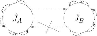
Figure 4: Approximations and modifications in the two-device model. Top: neglecting macroscopic back-action leads to generalised photodetection theory. Bottom: full quantum description of a device is restored by adding c-number sources to the model.

Structure of electromagnetic interactions in the outlined model is illustrated in Fig. 2. Assumed distinguishability of the devices leads to separation of the electromagnetic self-action problems for the devices from the problem of their electromagnetic interaction. For Fermi’s arrangement, this means that one may separate transients from the interaction of atoms via the field (cf. also endnote [26]). Furthermore, both in Fig. 1 and in Fig. 2 the electromagnetic interaction is shown as bidirectional. In Fermi’s arrangement, single-directedness is achieved by preparing the atoms in special quantum states (subject to reservations made in endnote [26]). Can one introduce single-directedness in the general arrangement of Fig. 2?

Formally, directedness of electromagnetic interaction is associated with the linear response function (also known as retarded Green function) of the free electromagnetic field. This quantity emerges if replacing the current operator in (6) by a c-number source $J_{\mathrm{e}}(x,t)$. This decouples matter from interaction. One can then calculate the linear response of the field [6, 27] (see also [28]),

$$\eqalign{\Delta_{\mathrm{R}}(x,x^{\prime},t-t^{\prime})=\frac{\delta\big{\langle}{\hat{\mathcal{A}}}(x,t)\big{\rangle}}{\delta J_{\mathrm{e}}(x^{\prime},t^{\prime})}\raisebox{-2.70003pt}{$\big{|}_{J_{\mathrm{e}}=0}$}=\frac{i}{\hbar}\theta(t-t^{\prime})\big{[}\hat{A}(x,t),\hat{A}(x^{\prime},t^{\prime})\big{]},}$$ (15)

where ${\hat{\mathcal{A}}}(x,t)$ is the Heisenberg field operator. The intermediate expression here is the definition of $\Delta_{\mathrm{R}}$, and the last one is Kubo’s formula for it [27]. Kubo’s proper expression contains quantum averaging of the commutator, which we omitted because the free-field commutator is a c-number anyway. Kubo’s formula may be inverted resulting in the wave quantisation relation [29],

$$\eqalign{\big{[}\hat{A}(x,t),\hat{A}(x^{\prime},t^{\prime})\big{]}=-i\hbar\big{[}\Delta_{\mathrm{R}}(x,x^{\prime},t-t^{\prime})-\Delta_{\mathrm{R}}(x^{\prime},x,t^{\prime}-t)\big{]}.}$$ (17)

Commutator (17) is all one needs to know about the field in order to construct the standard nonstationary perturbation solution to Hamiltonian (2). Technical means allowing one, firstly, to construct generalised perturbative series without specifying the model of matter, and, secondly, to rewrite it (series) in terms of $\Delta_{\mathrm{R}}$ is rather involved, but conceptually everything remains fairly simple. The resulting structure of electromagnetic interactions is illustrated in Fig. 3.

The roles the concept of single-directedness plays in the self-action and in the interaction problems are drastically different. In the case of self-action, both ends of $\Delta_{\mathrm{R}}$ are attached, so to speak, to the same electron. There is no way to control microscopic actions and back-actions associated with emitting and reabsorbing the field by matter at a microscopic level. Whereas in case of interaction, the signals travelling from device $A$ to device $B$ may be experimentally distinguished from those travelling from device $B$ to device $A$. This assumption concerns not only physics but also engineering. Physics implies that the situation is macroscopic (often termed mesoscopic, see endnote [30]): devices are distinguishable and separated by macroscopic distances, and all light beams may be controlled. Engineering takes care of such problems as, for instance, preventing light reflected off the detector input window from affecting the laser source.

Distinguishability of the incoming and outgoing electromagnetic signals for macroscopic electromagnetic devices are put to use in two ways. Dropping the signal travelling from device $B$ to device $A$ yields a generalised photodetection theory (Fig. 4, top). The dropped incoming wave may be restored by introducing c-number external sources into the Hamiltonian (Fig. 4, bottom). It is not immediately clear that c-number sources suffice to describe the incoming signal which in arrangement of Fig. 3 may be in a quantum state. This statement constitutes a generalisation of Sudarshan’s optical equivalence theorem [31] to arbitrary interacting systems.

The said generalisation of Sudarshan’s theorem is a particular case of a more general statement. Namely, in the formal structure corresponding to Fig. 3, Planck’s constant turns out to be eliminated from all relations between the quantised field and current [29]. Any such relation survives the limit $\hbar\to 0$ unchanged, and must therefore correspond to a particular relation of classical stochastic electrodynamics. The most natural expression of such quantum-classical corrrespondences emerges by mapping quantum relations into phase-space.

The order in which the aforesaid formal facts will be established is reversed compared to the logic of the above “pictorial argument.” The subject of the present paper is a solitary device interacting with c-number sources, as illustrated in Fig. 4, bottom. Phase-space mappings and quantum-classical correspondences will be the subject of paper [17]. Interactions of distinguishable devices, generalised photodetection theory and the optical equivalence theorem will be the subject of paper [18]. Apart from interaction (6), in all three papers we also look at its modification under the rotating wave approximation, and at how these two types of interaction coexist in a single model.

3 Generic model of a macroscopic electromagnetic device

3.1 RWA or no-RWA?

We consider a structural model of electromagnetic interaction where two sets of oscillator modes interact with a “quantum device.” The nature of the “device” may be arbitrary. For the modes, we assume two different types of coupling: a resonant electrical field-time-dipole coupling for one set, and a nonresonant potential-times-current coupling for the other. Later this will allow us to treat on an equal footing the light (of which the interaction with matter in quantum optics is commonly treated under the resonance, or rotating wave, approximation — RWA) and the photocurrent (which is a broad-band process and in no way is a subject to the RWA). We cannot just assume the RWA because we then lose the low frequency photocurrent modes. Nor are we really keen to keep our analyses without the RWA because this would essentially disconnect us from the quantum-optical paradigm. (To recognise the problem, the reader may try, for example, to reformulate Glauber’s photodetection theory [32, 33, 34] in terms of real fields rather than analytical signals.) There is no simple notational compromise because the number of dynamical variables in the two cases differ: one real field versus a pair of conjugates. We therefore see no other choice but to develop two versions of the theory in parallel.

To refer to physics rather than to formal techniques we shall talk about the broad-band (or nonresonant) and the narrow-band (or resonant) cases. Both the response transformations and the causal Wick theorems in the two cases differ. The broad-band case is a continuation of our papers [6, 7, 8] (and of paper [29]). The narrow-band case is an extension of paper [35], see also [36]. In paper [9] we referred to these cases as to the real and nonrelativistic ones, respectively. The change of terminology follows the change of motivation: advancing formal techniques in paper [9] versus understanding macroscopic quantum electrodynamics in this and forthcoming papers.

3.2 The Hamiltonian

Formally, we assume Hamiltonian (2) with some amendments. All field oscillators are divided in two groups of $M$ and $N-M$ modes, $1\leq M\leq N$, organised in two electromagnetic-field operators. The narrow-band, or resonant, field is,

$$\eqalign{\hat{E}(x,t)=i\sum_{\kappa=1}^{M}\sqrt{\frac{\hbar\omega_{\kappa}}{2}}u_{\kappa}(x)\hat{a}_{\kappa}\mathrm{e}^{-i(\omega_{\kappa}-\omega_{0})t},\\ \hat{E}^{{\dagger}}(x,t)=-i\sum_{\kappa=1}^{M}\sqrt{\frac{\hbar\omega_{\kappa}}{2}}u^{*}_{\kappa}(x)\hat{a}_{\kappa}^{{\dagger}}\mathrm{e}^{i(\omega_{\kappa}-\omega_{0})t},}$$ (20)

and the broad-band, or nonresonant, field is defined as,

$$\eqalign{\hat{A}(x,t)=\sum_{\kappa=M+1}^{N}\sqrt{\frac{\hbar}{2\omega_{\kappa}}}u_{\kappa}(x)\hat{a}_{\kappa}\mathrm{e}^{-i\omega_{\kappa}t}+\mathrm{H.c.}\,.}$$ (22)

In (20), $\omega_{0}$ is the characteristic optical carrier frequency. Other quantities in (20) and (22) have the same meaning as in section 2. For simplicity we assume that both fields depend on the same set of arguments. This restriction may be easily lifted.

For the resonant modes, their frequencies $\omega_{\kappa}$ are supposed to occupy a narrow band of frequencies centered at $\omega_{0}$. That is, $\hat{E}(x,t)$ and $\hat{E}^{{\dagger}}(x,t)$ are by definition slow amplitudes. However, this assumption is only important for physics. Formally, it may be disregraded, with the only exception of B. In the rest of the paper, $\omega_{0}$ is an arbitrary quantity which may safely be set to zero.

Electromagnetic interaction in (2) is also divided in two,

$$\eqalign{\hat{H}_{\mathrm{I}}(t)=\hat{H}_{\mathrm{I}}^{(1)}(t)+\hat{H}_{\mathrm{I}}^{(2)}(t).}$$ (24)

The narrow-band field interacts with the device according to the resonant Hamiltonian,

$$\eqalign{\hat{H}_{\mathrm{I}}^{(1)}(t)=-\int dx\big{[}\hat{D}(x,t)\hat{E}^{{\dagger}}(x,t)+\hat{D}(x,t)E^{*}_{\mathrm{e}}(x,t)+D_{\mathrm{e}}(x,t)\hat{E}^{{\dagger}}(x,t)\big{]}+\mathrm{H.c.}\,,}$$ (26)

while the broad-band field — according to the nonresonant Hamiltonian,

$$\eqalign{\hat{H}_{\mathrm{I}}^{(2)}(t)=-\int dx\big{[}\hat{J}(x,t)\hat{A}(x,t)+\hat{J}(x,t)A_{\mathrm{e}}(x,t)+J_{\mathrm{e}}(x,t)\hat{A}(x,t)\big{]}.}$$ (28)

The state of the system is given by equation (10). Motivation for introducing c-number sources into the interaction was elucidated in section 2.

Comments in the paragraph preceding equation (11) hold, except there is an additional operator $\hat{D}(x,t)$ characterising matter. Factorisation of the matter subspace will not be assumed till paper [18], so that equations (11), (12) and (13) do not apply.

Fields, currents and dipoles in equations (28) and (22) are interaction-picture operators. Their Heisenberg counterparts will be denoted by calligraphic letters as ${\hat{\mathcal{E}}}(x,t)$, ${\hat{\mathcal{A}}}(x,t)$, ${\hat{\mathcal{D}}}(x,t)$, and ${\hat{\mathcal{J}}}(x,t)$.

Hamiltonian (2) is a placeholder for all conceivable cases of electromagnetic interaction, from a single mode (with $M=N=1$) to relativistic quantum fields (with $M=0$ and $N\to\infty$). From our perspective, this Hamiltonian is a structural model of a quantum-optical experiment involving photodetection. Operators ${\hat{\mathcal{E}}}(x,t)$ and ${\hat{\mathcal{D}}}(x,t)$ describe optical interactions, while ${\hat{\mathcal{A}}}(x,t)$ and ${\hat{\mathcal{J}}}(x,t)$ express photovoltage and photocurrent. Without specifications, Hamiltonian (2) is a structural model of photodetector. By breaking the device into distinguishable components, we recover a structural model of the source-detector interaction, etc.

3.3 Operator orderings

Here we summarise definitions of operator orderings used in the paper. All definitions imply bosonic operators. Of importance to us are the normal and time orderings. The normal ordering puts $\hat{a}^{{\dagger}}$’s occuring in equation (2) to the left of $\hat{a}$’s,

$$\eqalign{{\mbox{\rm\boldmath$:$}}\hat{a}_{\kappa}\hat{a}_{\kappa^{\prime}}^{{\dagger}}{\mbox{\rm\boldmath$:$}}={\mbox{\rm\boldmath$:$}}\hat{a}_{\kappa^{\prime}}^{{\dagger}}\hat{a}_{\kappa}{\mbox{\rm\boldmath$:$}}=\hat{a}_{\kappa^{\prime}}^{{\dagger}}\hat{a}_{\kappa},}$$ (30)

etc. It is extended to the field operators (20), (22) by linearity. The time-orderings $T_{+}$ and $T_{-}$ put operators in the order of decreasing and increasing time arguments, respectively,

$$T_{+}{\hat{\mathcal{X}}}_{1}(t_{1}){\hat{\mathcal{X}}}_{2}(t_{2})\cdots{\hat{\mathcal{X}}}_{m}(t_{m})$$

$$\qquad=\sum_{\mathit{perms}}\theta(t_{1}-t_{2})\theta(t_{2}-t_{3})\cdots\theta(t_{m-1}-t_{m}){\hat{\mathcal{X}}}_{1}(t_{1}){\hat{\mathcal{X}}}_{2}(t_{2})\cdots{\hat{\mathcal{X}}}_{m}(t_{m}),$$ (31)

$$T_{-}{\hat{\mathcal{X}}}_{1}(t_{1}){\hat{\mathcal{X}}}_{2}(t_{2})\cdots{\hat{\mathcal{X}}}_{m}(t_{m})$$

$$\qquad=\sum_{\mathit{perms}}\theta(t_{1}-t_{2})\theta(t_{2}-t_{3})\cdots\theta(t_{m-1}-t_{m}){\hat{\mathcal{X}}}_{m}(t_{m})\cdots{\hat{\mathcal{X}}}_{2}(t_{2}){\hat{\mathcal{X}}}_{1}(t_{1}).$$ (32)

The sums are over all permutations of times $t_{1},\cdots,t_{m}$. Of use is the property,

$$\eqalign{{[T_{\pm}{\hat{\mathcal{X}}}_{1}(t_{1}){\hat{\mathcal{X}}}_{2}(t_{2})\cdots{\hat{\mathcal{X}}}_{m}(t_{m})]}^{{\dagger}}=T_{\mp}{\hat{\mathcal{X}}}_{1}^{{\dagger}}(t_{1}){\hat{\mathcal{X}}}_{2}^{{\dagger}}(t_{2})\cdots{\hat{\mathcal{X}}}_{m}^{{\dagger}}(t_{m}).}$$ (34)

It expresses the simple fact that Hermitian conjugation inverts the order of factors turning a $T_{+}$-ordered product into a $T_{-}$-ordered one, and vice versa. We note in passing that definitions like (31), (32) may cause mathematical problems, see the concluding remark in section IIIB of paper [9].

In formulae, the $T_{\pm}$-orderings mostly occur as double time ordered structures $T_{-}\cdots T_{+}\cdots$. Rather than visually keeping the operators under the $T_{\pm}$-orderings, one marks the operators with the _± indices and allows them to commute freely:

$$\eqalign{T_{-}{\hat{\mathcal{X}}}_{1}(t_{1})\cdots{\hat{\mathcal{X}}}_{m}(t_{m})\,T_{+}{\hat{\mathcal{Y}}}_{1}(t^{\prime}_{1})\cdots{\hat{\mathcal{Y}}}_{n}(t^{\prime}_{n})\\ \qquad=T_{C}{\hat{\mathcal{X}}}_{1-}(t_{1})\cdots{\hat{\mathcal{X}}}_{m-}(t_{m}){\hat{\mathcal{Y}}}_{1+}(t^{\prime}_{1})\cdots{\hat{\mathcal{Y}}}_{n+}(t^{\prime}_{n})\\ \qquad=T_{C}{\hat{\mathcal{Y}}}_{1+}(t^{\prime}_{1})\cdots{\hat{\mathcal{Y}}}_{n+}(t^{\prime}_{n}){\hat{\mathcal{X}}}_{1-}(t_{1})\cdots{\hat{\mathcal{X}}}_{m-}(t_{m}),}$$ (38)

etc. The _± indices serve only for ordering purposes and otherwise should be disregarded. Using $T_{C}$ results in a reduction of formulae in bulk which may be truly dramatic (compare, e.g., expressions for response functions in [7] and in [8]). In this paper we mostly use the $T_{C}$-ordering and revert to the double time ordering only where necessary.

3.4 Quantum Green functions

Quantized fields $\hat{E}(x,t)$ and $\hat{A}(x,t)$ enter all formulae through their Green functions. In either case, we define the retarded Green function and two contractions: the Feynman propagator, and one more kernel which emerges as a propagator in Perel-Keldysh’s diagram techniques (and which, strictly speaking, is not a Green function). For the resonant field, these quantities read, respectively,

$$G_{\mathrm{R}}(x,x^{\prime},t-t^{\prime})=\frac{i}{\hbar}\theta(t-t^{\prime})\big{\langle}0\big{|}\big{[}\hat{E}(x,t),\hat{E}^{{\dagger}}(x^{\prime},t^{\prime})\big{]}\big{|}0\big{\rangle},$$ (39)

$$G_{\mathrm{F}}(x,x^{\prime},t-t^{\prime})=\frac{i}{\hbar}\big{\langle}0\big{|}T_{+}\hat{E}(x,t)\hat{E}^{{\dagger}}(x^{\prime},t^{\prime})\big{|}0\big{\rangle},$$ (40)

$$G^{(+)}(x,x^{\prime},t-t^{\prime})=\frac{i}{\hbar}\big{\langle}0\big{|}\hat{E}(x,t)\hat{E}^{{\dagger}}(x^{\prime},t^{\prime})\big{|}0\big{\rangle}.$$ (41)

For the nonresonant field, they are,

$$\Delta_{\mathrm{R}}(x,x^{\prime},t-t^{\prime})=\frac{i}{\hbar}\theta(t-t^{\prime})\big{\langle}0\big{|}\big{[}\hat{A}(x,t),\hat{A}(x^{\prime},t^{\prime})\big{]}\big{|}0\big{\rangle},$$ (42)

$$\Delta_{\mathrm{F}}(x,x^{\prime},t-t^{\prime})=\frac{i}{\hbar}\big{\langle}0\big{|}T_{+}\hat{A}(x,t)\hat{A}(x^{\prime},t^{\prime})\big{|}0\big{\rangle},$$ (43)

$$\Delta^{(+)}(x,x^{\prime},t-t^{\prime})=\frac{i}{\hbar}\big{\langle}0\big{|}\hat{A}(x,t)\hat{A}(x^{\prime},t^{\prime})\big{|}0\big{\rangle}.$$ (44)

$T_{+}$ in (40) and (43) is the standard time-ordering defined by equation (31). Using (20), (22) we find the explicit formulae,

$$\eqalign{G^{(+)}(x,x^{\prime},t-t^{\prime})=i\sum_{\kappa=1}^{M}\frac{\omega_{\kappa}u_{\kappa}(x)u_{\kappa}^{*}(x^{\prime})\mathrm{e}^{-i\omega_{\kappa}(t-t^{\prime})}}{2},\\ \Delta^{(+)}(x,x^{\prime},t-t^{\prime})=i\sum_{\kappa=M+1}^{N}\frac{u_{\kappa}(x)u_{\kappa}^{*}(x^{\prime})\mathrm{e}^{-i\omega_{\kappa}(t-t^{\prime})}}{2\omega_{\kappa}}.}$$ (47)

Other kernels follow from the relations,

$$\eqalign{G_{\mathrm{R}}(x,x^{\prime},t-t^{\prime})=G_{\mathrm{F}}(x,x^{\prime},t-t^{\prime})=\theta(t-t^{\prime})G^{(+)}(x,x^{\prime},t-t^{\prime}),\\ \Delta_{\mathrm{R}}(x,x^{\prime},t-t^{\prime})=\theta(t-t^{\prime})\big{[}\Delta^{(+)}(x,x^{\prime},t-t^{\prime})-\Delta^{(+)}(x^{\prime},x,t^{\prime}-t)\big{]},\\ \Delta_{\mathrm{F}}(x,x^{\prime},t-t^{\prime})=\theta(t-t^{\prime})\Delta^{(+)}(x,x^{\prime},t-t^{\prime})+\theta(t^{\prime}-t)\Delta^{(+)}(x^{\prime},x,t^{\prime}-t).}$$ (51)

Definitions of the retarded Green functions (39) and (42) are Kubo’s formulae for linear response functions [27]. Definition of $\Delta_{\mathrm{R}}$ was discussed in section 2, cf. equation (15) and comments thereon. $G_{\mathrm{R}}$ is defined in a similar manner, setting $\hat{D}(x,t)=0$ in Hamiltonian (26) and then defining the linear response of the resonant field by the formula,

$$\eqalign{G_{\mathrm{R}}(x,x^{\prime},t-t^{\prime})=\frac{\delta\big{\langle}{\hat{\mathcal{E}}}(x,t)\big{\rangle}}{\delta D_{\mathrm{e}}(x^{\prime},t^{\prime})}\raisebox{-3.60004pt}{$\Big{|}_{D_{\mathrm{e}}=0}$}.}$$ (53)

Equation (39) is Kubo’s formula for $G_{\mathrm{R}}$. For more details on the linear response theory for free bosonic fields see papers [6, 28]. Commutators in (39) and (42) are c-numbers, so that the averaging may be dropped (in other words, response of a linear system does not depend on its state). In the other four definitions, this averaging matters.

3.5 Response transformation of contractions

All our results hinge on one observation: the propagators (contractions) may be expressed by the retarded Green functions [6, 9, 29, 35]. In the narrow-band case, this connection readily follows from (51),

$$\eqalign{G_{\mathrm{F}}(x,x^{\prime},t-t^{\prime})=G_{\mathrm{R}}(x,x^{\prime},t-t^{\prime}),\\ G^{(+)}(x,x^{\prime},t-t^{\prime})=G_{\mathrm{R}}(t-t^{\prime})-G_{\mathrm{R}}^{*}(x,x^{\prime},t^{\prime}-t).}$$ (56)

In the broad-band case, such connection is more involved. It happens to be an integral transformation [6, 9, 35],

$$\eqalign{\Delta_{\mathrm{F}}(x,x^{\prime},t-t^{\prime})=\Delta_{\mathrm{R}}^{(+)}(x,x^{\prime},t-t^{\prime})+\Delta_{\mathrm{R}}^{(+)}(x^{\prime},x,t^{\prime}-t),\\ \Delta^{(+)}(x,x^{\prime},t-t^{\prime})=\Delta_{\mathrm{R}}^{(+)}(x,x^{\prime},t-t^{\prime})-\Delta_{\mathrm{R}}^{(-)}(x^{\prime},x,t^{\prime}-t).}$$ (59)

The symbols ^(±) denote separation of the frequency-positive and negative parts of functions,

$$\eqalign{f(t)=f^{(+)}(t)+f^{(-)}(t),\\ f^{(\pm)}(t)=\int_{-\infty}^{+\infty}\frac{d\omega}{2\pi}\mathrm{e}^{-i\omega t}\theta(\pm\omega)f_{\omega},\\ f_{\omega}=\int_{-\infty}^{+\infty}dt\mathrm{e}^{i\omega t}f(t).}$$ (63)

The frequency-positive and negative parts are always defined with respect to native arguments of functions; so, $\Delta_{\mathrm{R}}^{(\pm)}(x^{\prime},x,t^{\prime}-t)$ in (59) are deciphered as $\Delta_{\mathrm{R}}^{(\pm)}(x^{\prime},x,t)\raisebox{-2.25002pt}{$|_{t\to t^{\prime}-t}$}$. For more details on this operation see paper [7], appendix A. Note that notation for $\Delta^{(+)}$ and $G^{(+)}$ is consistent with them being purely frequency-positive.

Equations (59) may be traced down to the wave quantisation formula (17), while (56) — to a similar formula for the narrow-band field,

$$\eqalign{\big{[}\hat{E}(x,t),\hat{E}^{{\dagger}}(x^{\prime},t^{\prime})\big{]}=-i\hbar\big{[}G_{\mathrm{R}}(x,x^{\prime},t-t^{\prime})-G^{*}_{\mathrm{R}}(x^{\prime},x,t^{\prime}-t)\big{]}.}$$ (65)

Note that $\Delta_{\mathrm{R}}$ is real, while $G_{\mathrm{R}}$ is complex. For more detals see papers [6, 9, 35].

3.6 Condensed notation

To keep the bulk of formulae under the lid and make their structure more transparent, we make extensive use of condensed notation,

$$fg=\int dxdtf(x,t)g(x,t),$$ (66)

$$fKg=\int dxdx^{\prime}dtdt^{\prime}f(x,t)K(x,x^{\prime},t-t^{\prime})g(x^{\prime},t^{\prime}),$$ (67)

$$(Kg)(x,t)=\int dx^{\prime}dt^{\prime}K(x,x^{\prime},t-t^{\prime})g(x^{\prime},t^{\prime}),$$ (68)

$$(fK)(x,t)=\int dx^{\prime}dt^{\prime}g(x^{\prime},t^{\prime})K(x^{\prime},x,t^{\prime}-t),$$ (69)

where $f(x,t)$ and $g(x,t)$ are c-number or q-number functions, and $K(x,x^{\prime},t-t^{\prime})$ is a c-number kernel. The “products” $fg$ and $fKg$ denote scalars, while $Kg$ and $fK$ — functions (fields).

4 Oscillators interacting with quantised current (the broad-band case)

4.1 The closed-time-loop formalism

Perturbative formulae for Hamiltonian (2) grow insufferably bulky. We therefore start from the relatively compact broad-band case. Formally, this corresponds to setting $M=0$ in equations (2)–(22).

To maintain connection with papers [6, 7, 8, 29, 35], we solve for the characteristic functional of products of the Heisenberg field and current operators, ${\hat{\mathcal{A}}}(x,t)$ and ${\hat{\mathcal{J}}}(x,t)$, ordered in the Schwinger-Perel-Keldysh closed-time-loop style [14, 15, 16],

$$\eqalign{\Xi({\eta}_{+},{\eta}_{-},{\zeta}_{+},{\zeta}_{-}|A_{\mathrm{e}},J_{\mathrm{e}})\\ \qquad=\big{\langle}T_{-}\exp\big{(}-i{\eta}_{-}{\hat{\mathcal{A}}}-i{\zeta}_{-}{\hat{\mathcal{J}}}\big{)}\,T_{+}\exp\big{(}i{\eta}_{+}{\hat{\mathcal{A}}}+i{\zeta}_{+}{\hat{\mathcal{J}}}\big{)}\big{\rangle}\\ \qquad=\big{\langle}T_{C}\exp\big{(}i{\eta}_{+}{\hat{\mathcal{A}}}_{+}-i{\eta}_{-}{\hat{\mathcal{A}}}_{-}+i{\zeta}_{+}{\hat{\mathcal{J}}}_{+}-i{\zeta}_{-}{\hat{\mathcal{J}}}_{-}\big{)}\big{\rangle},}$$ (73)

where $\eta_{\pm}(x,t)$ and $\zeta_{\pm}(x,t)$ are four independent complex functions. We use condensed notation (66). The averaging in (73) is over the initial (Heisenberg) state of the system,

$$\eqalign{\big{\langle}\cdots\big{\rangle}=\mathrm{Tr}\hat{\rho}(\cdots),}$$ (75)

where $\hat{\rho}$ is given by equation (10) and the ellipsis stands for an arbitrary operator. Definitions of operator orderings were summarised in section 3.3.

In this paper, we denote various characteristic functionals of $T_{C}$-ordered operator averages as $\Xi$, while the same functionals in causal variables will be denoted as $\Phi$. This agrees with notational conventions of paper [35]. Notation used in papers [6, 7, 8] is recovered replacing $\Xi\to\Phi$ and $\Phi\to\Phi_{\mathrm{R}}$. The reason for the change of notation compared to [6, 7, 8] is obvious: we attach quite a number of indices to the functionals, and an additional index would be a nuisance.

4.2 Dyson’s perturbative technique

As in papers [29, 35] we employ Dyson’s standard perturbative techniques [12]. We assume that the reader is familiar with the concept of S-matrix and its representation as a T-exponent,

$$\eqalign{{\hat{\mathcal{S}}}=T_{+}\exp\bigg{[}-\frac{i}{\hbar}\int dt\hat{H}(t)\bigg{]},}$$ (77)

where $\hat{H}(t)$ is the interaction Hamiltonian in the interaction picture. As in papers [6, 7, 8, 9], omitted integration limits imply the maximal possible area of integration: the whole time axis, the whole space, etc.

The key relation for us is the formula expressing time-ordered products of Heisenberg operators, ${\hat{\mathcal{X}}}_{1}(t_{1}),\cdots,{\hat{\mathcal{X}}}_{m}(t_{m})$, as time-ordered products of the same operators in the interaction picture, $\hat{X}_{1}(t_{1}),\cdots,\hat{X}_{m}(t_{m})$,

$$\eqalign{T_{+}{\hat{\mathcal{X}}}_{1}(t_{1})\cdots{\hat{\mathcal{X}}}_{m}(t_{m})={\hat{\mathcal{S}}}^{{\dagger}}T_{+}{\hat{\mathcal{S}}}\hat{X}_{1}(t_{1})\cdots\hat{X}_{m}(t_{m}).}$$ (79)

Detailed derivation of this formula may be found, for instance, in Schweber’s textbook [12]. Uncharacteristically for ever-so-thorough Schweber, derivation in [12] disregards the ${\hat{\mathcal{S}}}^{{\dagger}}$ factor; for the necessary amendments see our paper [8], section 5.2. Taking the adjoint of equation (79) and using equation (34) we also obtain,

$$\eqalign{T_{-}{\hat{\mathcal{X}}}_{1}(t_{1})\cdots{\hat{\mathcal{X}}}_{m}(t_{m})=\big{[}T_{-}{\hat{\mathcal{S}}}^{{\dagger}}\hat{X}_{1}(t_{1})\cdots\hat{X}_{m}(t_{m})\big{]}{\hat{\mathcal{S}}}.}$$ (81)

Square brackets mark the region to which the ordering applies.

Equations (77)–(81) imply that the S-matrix is regarded a functional of the operators $\hat{A}(x,t)$ and $\hat{J}(x,t)$. The reader should keep this in mind to avoid confusion and misunderstanding. For details see Vasil’ev [13].

In the case at hand, the S-matrix and its inverse read,

$${\hat{\mathcal{S}}}=T_{+}\exp\bigg{[}\frac{i}{\hbar}\big{(}\hat{A}\hat{J}+A_{\mathrm{e}}\hat{J}+\hat{A}J_{\mathrm{e}}\big{)}\bigg{]},$$ (82)

$${\hat{\mathcal{S}}}^{{\dagger}}=T_{-}\exp\bigg{[}-\frac{i}{\hbar}\big{(}\hat{A}\hat{J}+A_{\mathrm{e}}\hat{J}+\hat{A}J_{\mathrm{e}}\big{)}\bigg{]},$$ (83)

where $\hat{A}(x,t)$ and $\hat{J}(x,t)$ are the field and current operators in the interaction picture. The former is given by (22), while the latter is just assumed to be known. We continue using condensed notation (66). Applying equations (79), (81) we obtain,

$$T_{+}\exp\big{(}i\eta_{+}{\hat{\mathcal{A}}}+i\zeta_{+}{\hat{\mathcal{J}}}\big{)}$$

$$\qquad={\hat{\mathcal{S}}}^{{\dagger}}T_{+}\exp\big{(}i\eta_{+}\hat{A}+i\zeta_{+}\hat{J}\big{)}\exp\bigg{[}\frac{i}{\hbar}\big{(}\hat{A}\hat{J}+A_{\mathrm{e}}\hat{J}+\hat{A}J_{\mathrm{e}}\big{)}\bigg{]},$$ (84)

$$T_{-}\exp\big{(}-i\eta_{-}{\hat{\mathcal{A}}}-i\zeta_{-}{\hat{\mathcal{J}}}\big{)}$$

$$\qquad=\bigg{\{}T_{-}\exp\big{(}-i\eta_{-}\hat{A}-i\zeta_{-}\hat{J}\big{)}\exp\bigg{[}-\frac{i}{\hbar}\big{(}\hat{A}\hat{J}+A_{\mathrm{e}}\hat{J}+\hat{A}J_{\mathrm{e}}\big{)}\bigg{]}\bigg{\}}{\hat{\mathcal{S}}},$$ (85)

Unlike in equations (79), (81), in equations (82)–(85) the distinction between operators ${\hat{\mathcal{S}}}$ and ${\hat{\mathcal{S}}}^{{\dagger}}$ and their representation as time-ordered operator functionals is explicitly maintained. When substituting equations (84), (85) into (73), the ${\hat{\mathcal{S}}}^{{\dagger}}$ and ${\hat{\mathcal{S}}}$ factors cancel each other,

$$\eqalign{{\hat{\mathcal{S}}}{\hat{\mathcal{S}}}^{{\dagger}}=\hat{1},}$$ (87)

and we have,

$$\Xi\big{(}{\eta}_{+},{\eta}_{-},{\zeta}_{+},{\zeta}_{-}\big{|}J_{\mathrm{e}},A_{\mathrm{e}}\big{)}$$

$$\qquad=\bigg{\langle}T_{-}\exp\big{(}-i\eta_{-}\hat{A}-i\zeta_{-}\hat{J}\big{)}\exp\bigg{[}-\frac{i}{\hbar}\big{(}\hat{A}\hat{J}+A_{\mathrm{e}}\hat{J}+\hat{A}J_{\mathrm{e}}\big{)}\bigg{]}$$

$$\qquad\qquad\times T_{+}\exp\big{(}i\eta_{+}\hat{A}+i\zeta_{+}\hat{J}\big{)}\exp\bigg{[}\frac{i}{\hbar}\big{(}\hat{A}\hat{J}+A_{\mathrm{e}}\hat{J}+\hat{A}J_{\mathrm{e}}\big{)}\bigg{]}\bigg{\rangle}.$$ (88)

The same in terms of $T_{C}$-ordering reads,

$$\Xi\big{(}{\eta}_{+},{\eta}_{-},{\zeta}_{+},{\zeta}_{-}\big{|}J_{\mathrm{e}},A_{\mathrm{e}}\big{)}=\bigg{\langle}T_{C}\exp\big{(}i\eta_{+}\hat{A}_{+}-i\eta_{-}\hat{A}_{-}+i\zeta_{+}\hat{J}_{+}-i\zeta_{-}\hat{J}_{-}\big{)}$$

$$\qquad\times\exp\bigg{[}\frac{i}{\hbar}\big{(}\hat{A}_{+}\hat{J}_{+}+A_{\mathrm{e}}\hat{J}_{+}+\hat{A}_{+}J_{\mathrm{e}}\big{)}\bigg{]}\exp\bigg{[}-\frac{i}{\hbar}\big{(}\hat{A}_{-}\hat{J}_{-}+A_{\mathrm{e}}\hat{J}_{-}+\hat{A}_{-}J_{\mathrm{e}}\big{)}\bigg{]}\bigg{\rangle}.$$ (89)

Grouping of arguments in this formula is an allusion to its “ancestors:” equations (73), (82) and (83).

4.3 Wick’s theorem and elimination of field operators

In the standard techniques of quantum field theory [12, 13], the next step is applying Wick’s theorem [10] to equation (89). Wick’s theorem allows one to rewrite time-ordered operator structures in a normally-ordered form (for definitions of operator orderings see section 3.3). This comes especially handy if the initial state of the system is vacuum.

The interaction-picture operators $\hat{A}(x,t)$ and $\hat{J}(x,t)$ are defined in two orthogonal subspaces and may be manipulated independently. Due to assumed factorisation of the density matrix, this equally applies to quantum averaging. We therefore apply Wick’s theorem only to the field operators in (89), keeping the current operators “as are.”

We employ the functional (Hori’s [11]) form of Wick’s theorem (the Hori-Wick theorem, for short). It is discussed by Vasil’ev [13] and in our paper [9]. The directly applicable case is that of real field, see paper [9], section VIII. The Hori-Wick theorem for a real field reads,

$$\eqalign{T_{C}\mathcal{F}(\hat{A}_{+},\hat{A}_{-})={\mbox{\rm\boldmath$:$}}\mathcal{F}_{N}(\hat{A},\hat{A}){\mbox{\rm\boldmath$:$}},\\ \mathcal{F}_{N}(A_{+},A_{-})=\exp\mathcal{Z}_{C}\bigg{(}\frac{\delta}{\delta A_{+}},\frac{\delta}{\delta A_{-}}\bigg{)}\mathcal{F}(A_{+},A_{-}),}$$ (92)

where $A_{\pm}(x,t)$ are auxiliary c-number functional arguments, and $\mathcal{F}(\cdot,\cdot)$ is an arbitrary c-number functional. The reordering form $\mathcal{Z}_{C}(\cdot,\cdot)$ is a functional bilinear form where the kernels are contractions, (with $f_{\pm}(x,t)$ being auxiliary functional arguments)

$$\eqalign{\mathcal{Z}_{C}\big{(}f_{+},f_{-}\big{)}=-\frac{i\hbar}{2}f_{+}\Delta_{\mathrm{F}}f_{+}+\frac{i\hbar}{2}f_{-}\Delta_{\mathrm{F}}^{*}f_{-}-i\hbar f_{-}\Delta^{(+)}f_{+}.}$$ (94)

We use notation (67). Differentiations are carried out using the relations,

$$\eqalign{\frac{\delta A_{+}(x,t)}{\delta A_{+}(x^{\prime},t^{\prime})}=\frac{\delta A_{-}(x,t)}{\delta A_{-}(x^{\prime},t^{\prime})}=\delta(x-x^{\prime})\delta(t-t^{\prime}),\\ \frac{\delta A_{+}(x,t)}{\delta A_{-}(x^{\prime},t^{\prime})}=\frac{\delta A_{-}(x,t)}{\delta A_{+}(x^{\prime},t^{\prime})}=0.}$$ (97)

Note that under the normal ordering in equation (92) the _± indices of the operators are dropped as irrelevant.

For any functional $\mathcal{F}_{N}(\cdot,\cdot)$,

$$\eqalign{\big{\langle}0\big{|}{\mbox{\rm\boldmath$:$}}\mathcal{F}_{N}(\hat{A},\hat{A}){\mbox{\rm\boldmath$:$}}\big{|}0\big{\rangle}=\mathcal{F}_{N}(0,0),}$$ (99)

and we find,

$$\Xi\big{(}{\eta}_{+},{\eta}_{-},{\zeta}_{+},{\zeta}_{-}\big{|}J_{\mathrm{e}},A_{\mathrm{e}}\big{)}=\exp\mathcal{Z}_{C}\bigg{(}\frac{\delta}{\delta A_{+}},\frac{\delta}{\delta A_{-}}\bigg{)}$$

$$\qquad\times\exp\bigg{[}i\bigg{(}\eta_{+}+\frac{J_{\mathrm{e}}}{\hbar}\bigg{)}A_{+}-i\bigg{(}\eta_{-}+\frac{J_{\mathrm{e}}}{\hbar}\bigg{)}A_{-}\bigg{]}$$

$$\qquad\times\mathrm{Tr}\hat{\rho}_{\mathrm{dev}}T_{C}\exp\bigg{[}i\hat{J}_{+}\bigg{(}\frac{A_{+}+A_{\mathrm{e}}}{\hbar}+\zeta_{+}\bigg{)}-i\hat{J}_{-}\bigg{(}\frac{A_{-}+A_{\mathrm{e}}}{\hbar}+\zeta_{-}\bigg{)}\bigg{]}\raisebox{-3.60004pt}{$\Big{|}_{A_{\pm}=0}$}.$$ (100)

The necessary and sufficient information about the device is thus collected in the functional,

$$\eqalign{\Xi_{\mathrm{dev}}^{\mathrm{I}}\big{(}\zeta_{+},\zeta_{-}\big{)}=\mathrm{Tr}\hat{\rho}_{\mathrm{dev}}T_{C}\exp\big{(}i\zeta_{+}\hat{J}_{+}-i\zeta_{-}\hat{J}_{-}\big{)}.}$$ (102)

With it we have,

$$\Xi\big{(}{\eta}_{+},{\eta}_{-},{\zeta}_{+},{\zeta}_{-}\big{|}J_{\mathrm{e}},A_{\mathrm{e}}\big{)}=\exp\mathcal{Z}_{C}\bigg{(}\frac{\delta}{\delta A_{+}},\frac{\delta}{\delta A_{-}}\bigg{)}$$

$$\qquad\times\exp\bigg{[}i\bigg{(}\eta_{+}+\frac{J_{\mathrm{e}}}{\hbar}\bigg{)}A_{+}-i\bigg{(}\eta_{-}+\frac{J_{\mathrm{e}}}{\hbar}\bigg{)}A_{-}\bigg{]}$$

$$\qquad\times\Xi_{\mathrm{dev}}^{\mathrm{I}}\bigg{(}\frac{A_{+}+A_{\mathrm{e}}}{\hbar}+\zeta_{+},\frac{A_{-}+A_{\mathrm{e}}}{\hbar}+\zeta_{-}\bigg{)}\raisebox{-3.60004pt}{$\Big{|}_{A_{\pm}=0}$}.$$ (103)

4.4 Response transformations revisited

We are interested not in functional $\Xi$ as such but in its response transformation [6, 7, 8], (cf. the closing remark in section 4.1)

$$\eqalign{\Phi\big{(}\eta,\zeta\big{|}j_{\mathrm{e}},a_{\mathrm{e}}\big{|}J_{\mathrm{e}},A_{\mathrm{e}}\big{)}=\Xi\big{(}{\eta}_{+},{\eta}_{-},{\zeta}_{+},{\zeta}_{-}\big{|}J_{\mathrm{e}},A_{\mathrm{e}}\big{)}\raisebox{-2.25002pt}{$|_{\mathrm{c.v.}}$},}$$ (105)

where c.v. (short for causal variables [9, 35]) refers to the response substitutions [6, 7, 8, 9],

$$\eta_{\pm}(x,t)=\frac{j_{\mathrm{e}}(x,t)}{\hbar}\pm\eta^{(\mp)}(x,t),$$ (106)

$$\zeta_{\pm}(x,t)=\frac{a_{\mathrm{e}}(x,t)}{\hbar}\pm\zeta^{(\mp)}(x,t).$$ (107)

The frequency-positive and negative parts are defined by equation (63). Formulae for the causal variables are,

$${\eqalign{\eta(x,t)=\eta_{+}(x,t)-\eta_{-}(x,t),\qquad j_{\mathrm{e}}(x,t)=\hbar\big{[}\eta_{+}^{(+)}(x,t)+\eta_{-}^{(-)}(x,t)\big{]},}}$$ (109)

$${\eqalign{\zeta(x,t)=\zeta_{+}(x,t)-\zeta_{-}(x,t),\qquad a_{\mathrm{e}}(x,t)=\hbar\big{[}\zeta_{+}^{(+)}(x,t)+\zeta_{-}^{(-)}(x,t)\big{]}.}}$$ (111)

Equations (106), (107) and (109), (111) are mutually inverse, showing that these formulae constitute a genuine change of functional variables. Response substitutions are inherently related to equations (59). For details see our paper [6].

4.5 The causal Wick theorem revisited

For the two exponents in (103), the laws of transformation were worked out in paper [9], section VIIIB. With $\Xi_{\mathrm{dev}}^{\mathrm{I}}=1$ and $J_{\mathrm{e}}(x,t)=0$, equation (103) reduces to the “test-case formula” (104) in paper [9]. To rewrite that relation in causal variables we applied additional response substitution,

$$\eqalign{A_{\pm}(x,t)=a_{\mathrm{e}}^{\prime}(x,t)\pm\hbar\zeta^{\prime(\mp)}(x,t).}$$ (113)

Variables $a_{\mathrm{e}}^{\prime}(x,t)$, $\zeta^{\prime}(x,t)$ are given by the formulae,

$$\eqalign{\zeta^{\prime}(x,t)=\frac{A_{+}(x,t)-A_{-}(x,t)}{\hbar},\qquad a_{\mathrm{e}}^{\prime}(x,t)=A_{+}^{(+)}(x,t)+A_{-}^{(-)}(x,t).}$$ (115)

Equations (113), (115) are a rescaled version of (107), (111): they turn into the latter if we define,

$$\eqalign{\zeta_{\pm}^{\prime}(x,t)=\frac{A_{\pm}(x,t)}{\hbar}.}$$ (117)

Primes keep variables (115) distinct from (111).

In causal variables,

$$\eqalign{\bigg{[}i\bigg{(}\eta_{+}+\frac{J_{\mathrm{e}}}{\hbar}\bigg{)}A_{+}-i\bigg{(}\eta_{-}+\frac{J_{\mathrm{e}}}{\hbar}\bigg{)}A_{-}\bigg{]}\raisebox{-3.60004pt}{$\Big{|}_{{\mathrm{c.v.}}}$}=\eta a_{\mathrm{e}}^{\prime}+\zeta^{\prime}\big{(}j_{\mathrm{e}}+J_{\mathrm{e}}\big{)},}$$ (119)

and

$$\eqalign{\mathcal{Z}_{C}\bigg{(}\frac{\delta}{\delta A_{+}},\frac{\delta}{\delta A_{-}}\bigg{)}\raisebox{-3.60004pt}{$\Big{|}_{{\mathrm{c.v.}}}$}=-i\frac{\delta}{\delta a_{\mathrm{e}}^{\prime}}\Delta_{\mathrm{R}}\frac{\delta}{\delta\zeta^{\prime}},}$$ (121)

where we use condensed notation (66), (67).

4.6 Closed perturbative formula in causal variables

As to the functional $\Xi_{\mathrm{dev}}^{\mathrm{I}}$, we define,

$$\eqalign{\Phi_{\mathrm{dev}}^{\mathrm{I}}\big{(}\zeta\big{|}a_{\mathrm{e}}\big{)}=\Xi_{\mathrm{dev}}^{\mathrm{I}}({\zeta}_{+},{\zeta}_{-})\raisebox{-2.25002pt}{$|_{\mathrm{c.v.}}$},}$$ (123)

where c.v. refers to substitution (111). Combining (111) and (113) it is easy to show that,

$$\frac{A_{\mathrm{e}}(x,t)+A_{\pm}(x,t)}{\hbar}+\zeta_{\pm}(x,t)$$

$$\qquad=\frac{A_{\mathrm{e}}(x,t)+a_{\mathrm{e}}(x,t)+a_{\mathrm{e}}^{\prime}(x,t)}{\hbar}\pm\zeta^{(\mp)}(x,t)\pm\zeta^{{}^{\prime}(\mp)}(x,t),$$ (124)

hence

$$\eqalign{\Xi_{\mathrm{dev}}^{\mathrm{I}}\bigg{(}\frac{A_{\mathrm{e}}+A_{+}}{\hbar}+\zeta_{+},\frac{A_{\mathrm{e}}+A_{-}}{\hbar}+\zeta_{-}\bigg{)}\raisebox{-3.60004pt}{$\Big{|}_{\mathrm{c.v.}}$}=\Phi_{\mathrm{dev}}^{\mathrm{I}}\big{(}\zeta+\zeta^{\prime}\big{|}A_{\mathrm{e}}+a_{\mathrm{e}}+a_{\mathrm{e}}^{\prime}\big{)}.}$$ (126)

Putting equations (119), (121) and (126) together we obtain the relation sought,

$$\Phi\big{(}\eta,\zeta\big{|}j_{\mathrm{e}},a_{\mathrm{e}}\big{|}J_{\mathrm{e}},A_{\mathrm{e}}\big{)}=\exp\bigg{(}-i\frac{\delta}{\delta a_{\mathrm{e}}^{\prime}}\Delta_{\mathrm{R}}\frac{\delta}{\delta\zeta^{\prime}}\bigg{)}$$

$$\qquad\times\exp\big{[}i\eta a_{\mathrm{e}}^{\prime}+i\zeta^{\prime}\big{(}j_{\mathrm{e}}+J_{\mathrm{e}}\big{)}\big{]}\Phi_{\mathrm{dev}}^{\mathrm{I}}\big{(}\zeta+\zeta^{\prime}\big{|}A_{\mathrm{e}}+a_{\mathrm{e}}+a_{\mathrm{e}}^{\prime}\big{)}\raisebox{-2.25002pt}{$|_{\zeta^{\prime}=a_{\mathrm{e}}^{\prime}=0}$}.$$ (127)

The generalised consistency condition [7, 8],

$$\Phi\big{(}\eta,\zeta\big{|}j_{\mathrm{e}},a_{\mathrm{e}}\big{|}J_{\mathrm{e}},A_{\mathrm{e}}\big{)} =\Phi\big{(}\eta,\zeta\big{|}j_{\mathrm{e}}+J_{\mathrm{e}},a_{\mathrm{e}}+A_{\mathrm{e}}\big{|}0,0\big{)}\equiv\Phi\big{(}\eta,\zeta\big{|}j_{\mathrm{e}}+J_{\mathrm{e}},a_{\mathrm{e}}+A_{\mathrm{e}}\big{)},$$ (128)

is evident in (127).

In what follows, we set $A_{\mathrm{e}}(x,t)$ and $J_{\mathrm{e}}(x,t)$ to zero. Relations with sources, which are important for physics, may always be restored replacing $a_{\mathrm{e}}(x,t)\to a_{\mathrm{e}}(x,t)+A_{\mathrm{e}}(x,t)$ and $j_{\mathrm{e}}(x,t)\to j_{\mathrm{e}}(x,t)+J_{\mathrm{e}}(x,t)$.

4.7 Dressing the current

Unlike in the linear case [9], finding a closed solution to (127) is certainly impossible. One can, however, reduce (127) to the functional,

$$\eqalign{\Phi_{\mathrm{dev}}\big{(}\zeta\big{|}a_{\mathrm{e}}\big{)}=\Phi\big{(}0,\zeta\big{|}0,a_{\mathrm{e}}\big{)}=\Phi\big{(}0,\zeta\big{|}0,a_{\mathrm{e}}\big{|}0,0\big{)},}$$ (130)

cf. equation (128). This functional expresses the properties of the Heisenberg current operator (physical, or “dressed,” current). A perturbative formula for $\Phi_{\mathrm{dev}}$ is given by equation (127) with $\eta(x,t)=j_{\mathrm{e}}(x,t)=A_{\mathrm{e}}(x,t)=J_{\mathrm{e}}(x,t)=0$,

$$\eqalign{\Phi_{\mathrm{dev}}\big{(}\zeta\big{|}a_{\mathrm{e}}\big{)}=\exp\bigg{(}-i\frac{\delta}{\delta a_{\mathrm{e}}}\Delta_{\mathrm{R}}\frac{\delta}{\delta\zeta}\bigg{)}\Phi_{\mathrm{dev}}^{\mathrm{I}}\big{(}\zeta\big{|}a_{\mathrm{e}}\big{)}.}$$ (132)

Functional $\Phi_{\mathrm{dev}}^{\mathrm{I}}$ expresses the properties of the interaction-pictire current operator (“bare” current). Equation (132) thus expresses “dressing” of the current operator by the electromagnetic interaction.

Finding the dressed current is the hard part of the problem. Vast majority of technical developments in quantum field theory, condensed matter physics and quantum optics are in essense attempts to approximate equation (132) or its counterparts. Connections between equation (132) and diagram techniques are elucidated by Vasil’ev [13]. In A we construct a formal solution to (132) in terms of a diagram expansion. That (132) may be used as an alternative entry point to phase-space techniques was shown in paper [35].

4.8 Solution in terms of dressed current

Assuming that equation (132) is solved, full electromagnetic properties of the device follow with ease. We employ the formula,

$$\eqalign{\exp\bigg{(}f\frac{\delta}{\delta g}\bigg{)}\exp\big{(}igh\big{)}=\exp\big{(}igh\big{)}\exp\bigg{[}f\bigg{(}\frac{\delta}{\delta g}+ih\bigg{)}\bigg{]},}$$ (134)

where $f(x,t)$, $g(x,t)$ and $h(x,t)$ are c-number functions. It can be verified, e.g., expanding all exponents in Taylor series. With it we can pull $\exp\big{(}i\eta a_{\mathrm{e}}^{\prime}+i\zeta^{\prime}j_{\mathrm{e}}\big{)}$ from under the differentiation resulting in,

$$\Phi\big{(}\eta,\zeta\big{|}j_{\mathrm{e}},a_{\mathrm{e}}\big{)}=\exp\big{(}i\eta a_{\mathrm{e}}^{\prime}+i\zeta^{\prime}j_{\mathrm{e}}\big{)}$$

$$\qquad\times\exp\bigg{[}-i\bigg{(}\frac{\delta}{\delta a_{\mathrm{e}}^{\prime}}+i\eta\bigg{)}\Delta_{\mathrm{R}}\bigg{(}\frac{\delta}{\delta\zeta^{\prime}}+ij_{\mathrm{e}}\bigg{)}\bigg{]}\Phi_{\mathrm{dev}}^{\mathrm{I}}\big{(}\zeta+\zeta^{\prime}\big{|}a_{\mathrm{e}}+a_{\mathrm{e}}^{\prime}\big{)}\raisebox{-2.25002pt}{$|_{\zeta^{\prime}=a_{\mathrm{e}}^{\prime}=0}$}.$$ (135)

Setting $\zeta^{\prime}(x,t)$ and $a_{\mathrm{e}}^{\prime}(x,t)$ to zero we find,

$$\eqalign{\Phi\big{(}\eta,\zeta\big{|}j_{\mathrm{e}},a_{\mathrm{e}}\big{)}=\exp\bigg{[}-i\bigg{(}\frac{\delta}{\delta a_{\mathrm{e}}}+i\eta\bigg{)}\Delta_{\mathrm{R}}\bigg{(}\frac{\delta}{\delta\zeta}+ij_{\mathrm{e}}\bigg{)}\bigg{]}\Phi_{\mathrm{dev}}^{\mathrm{I}}\big{(}\zeta\big{|}a_{\mathrm{e}}\big{)}.}$$ (137)

Bilinearity of the form in the exponent allows us to write,

$$\exp\bigg{[}-i\bigg{(}\frac{\delta}{\delta a_{\mathrm{e}}}+i\eta\bigg{)}\Delta_{\mathrm{R}}\bigg{(}\frac{\delta}{\delta\zeta}+ij_{\mathrm{e}}\bigg{)}\bigg{]}$$

$$\qquad=\exp\big{(}i\eta\Delta_{\mathrm{R}}j_{\mathrm{e}}\big{)}\exp\bigg{(}\frac{\delta}{\delta a_{\mathrm{e}}}\Delta_{\mathrm{R}}j_{\mathrm{e}}\bigg{)}\exp\bigg{(}\eta\Delta_{\mathrm{R}}\frac{\delta}{\delta\zeta}\bigg{)}\exp\bigg{(}-i\frac{\delta}{\delta a_{\mathrm{e}}}\Delta_{\mathrm{R}}\frac{\delta}{\delta\zeta}\bigg{)}.$$ (138)

The last factor here is the dressing operator, cf. equation (132). The second and the third ones are functional shift operators. Applying the dressing and the two shifts to $\Phi_{\mathrm{dev}}^{\mathrm{I}}$ we obtain,

$$\Phi\big{(}\eta,\zeta\big{|}j_{\mathrm{e}},a_{\mathrm{e}}\big{|}J_{\mathrm{e}},A_{\mathrm{e}}\big{)}$$

$$\qquad=\exp\big{[}i\eta\Delta_{\mathrm{R}}\big{(}j_{\mathrm{e}}+J_{\mathrm{e}}\big{)}\big{]}\Phi_{\mathrm{dev}}\big{(}\zeta+\eta\Delta_{\mathrm{R}}\big{|}a_{\mathrm{e}}+A_{\mathrm{e}}+\Delta_{\mathrm{R}}\big{(}j_{\mathrm{e}}+J_{\mathrm{e}}\big{)}\big{)},$$ (139)

where we use abbreviated notation of equations (68) and (69). In equation (139) the external sources are restored. Without the device ($\Phi_{\mathrm{dev}}=1$) and with $J_{\mathrm{e}}(x,t)=0$ we recover the test-case formula of paper [9],

$$\eqalign{\Phi_{\mathrm{vac}}\big{(}\eta\big{|}j_{\mathrm{e}}\big{)}=\exp\big{(}i\eta\Delta_{\mathrm{R}}j_{\mathrm{e}}\big{)}.}$$ (141)

The physical content of equations (132) and (139) is a subject of forthcoming papers.

5 Oscillators interacting with quantised dipole (the narrow-band case)

5.1 Closed-time-loop formalism and perturbation theory

We now consider the second generic case: a quantised dipole interacting with a set of oscillators under the RWA. Formally, one sets $M=N$ in equations (20), (22). To a large extent, amendments to the broad-band case reduce to considering two fields, ${\hat{\mathcal{A}}}(x,t)\to{\hat{\mathcal{E}}}(x,t),{\hat{\mathcal{E}}}^{{\dagger}}(x,t)$, and two “currents,” ${\hat{\mathcal{J}}}(x,t)\to{\hat{\mathcal{D}}}(x,t),{\hat{\mathcal{D}}}^{{\dagger}}(x,t)$, with ${\hat{\mathcal{E}}}(x,t)$ coupled to ${\hat{\mathcal{D}}}^{{\dagger}}(x,t)$ and ${\hat{\mathcal{E}}}^{{\dagger}}(x,t)$ to ${\hat{\mathcal{D}}}(x,t)$. We remind that ${\hat{\mathcal{E}}}(x,t)$, ${\hat{\mathcal{D}}}(x,t)$ are Heisenberg counterparts of the interaction-picture operators $\hat{E}(x,t)$, $\hat{D}(x,t)$; $\hat{E}(x,t)$ is given by equation (20) and $\hat{D}(x,t)$ is “just assumed known.” Consequently all arguments in characteristic functionals also double, $\eta_{\pm}(x,t)\to\mu_{\pm}(x,t),\bar{\mu}_{\pm}(x,t)$, $\zeta_{\pm}(x,t)\to\nu_{\pm}(x,t),\bar{\nu}_{\pm}(x,t)$, etc. The basic object of the theory, the characteristic functional of the $T_{C}$-ordered products of the Heisenberg field and dipole operators, reads, (cf. the closing remark in section 4.1)

$$\Xi\big{(}\bar{\mu}_{+},\mu_{+},\bar{\mu}_{-},\mu_{-},\bar{\nu}_{+},\nu_{+},\bar{\nu}_{-},\nu_{-}\big{|}D_{\mathrm{e}},D_{\mathrm{e}}^{*},E_{\mathrm{e}},E_{\mathrm{e}}^{*}\big{)}$$

$$\qquad=\Big{\langle}T_{C}\exp\big{(}i\bar{\mu}_{+}{\hat{\mathcal{E}}}_{+}+i\mu_{+}{\hat{\mathcal{E}}}_{+}^{{\dagger}}-i\bar{\mu}_{-}{\hat{\mathcal{E}}}_{-}-i\mu_{-}{\hat{\mathcal{E}}}_{-}^{{\dagger}}$$

$$\qquad\qquad+i\bar{\nu}_{+}{\hat{\mathcal{D}}}_{+}+i\nu_{+}{\hat{\mathcal{D}}}_{+}^{{\dagger}}-i\bar{\nu}_{-}{\hat{\mathcal{D}}}_{-}-i\nu_{-}{\hat{\mathcal{D}}}_{-}^{{\dagger}}\big{)}\Big{\rangle}.$$ (142)

We again employ condensed notation (66). The S-matrix and its adjoint now are,

$${\hat{\mathcal{S}}}=T_{+}\exp\bigg{\{}\frac{i}{\hbar}\big{[}\hat{E}\hat{D}^{{\dagger}}+E_{\mathrm{e}}\hat{D}^{{\dagger}}+\hat{E}\hat{D}_{\mathrm{e}}^{*}+\hat{E}^{{\dagger}}\hat{D}+E_{\mathrm{e}}^{*}\hat{D}+\hat{E}^{{\dagger}}\hat{D}_{\mathrm{e}}\big{]}\bigg{\}},$$ (143)

$${\hat{\mathcal{S}}}^{{\dagger}}=T_{-}\exp\bigg{\{}-\frac{i}{\hbar}\big{[}\hat{E}\hat{D}^{{\dagger}}+E_{\mathrm{e}}\hat{D}^{{\dagger}}+\hat{E}\hat{D}_{\mathrm{e}}^{*}+\hat{E}^{{\dagger}}\hat{D}+E_{\mathrm{e}}^{*}\hat{D}+\hat{E}^{{\dagger}}\hat{D}_{\mathrm{e}}\big{]}\bigg{\}},$$ (144)

By the same means as equation (89) was obtained we find a perturbative formula,

$$\Xi\big{(}\bar{\mu}_{+},\mu_{+},\bar{\mu}_{-},\mu_{-},\bar{\nu}_{+},\nu_{+},\bar{\nu}_{-},\nu_{-}\big{|}D_{\mathrm{e}},D_{\mathrm{e}}^{*},E_{\mathrm{e}},E_{\mathrm{e}}^{*}\big{)}$$

$$\qquad=\bigg{\langle}T_{C}\exp\big{(}i\bar{\mu}_{+}\hat{E}_{+}+i\mu_{+}\hat{E}_{+}^{{\dagger}}-i\bar{\mu}_{-}\hat{E}_{-}-i\mu_{-}\hat{E}_{-}^{{\dagger}}$$

$$\qquad\qquad\qquad\qquad\qquad+i\bar{\nu}_{+}\hat{D}_{+}+i\nu_{+}\hat{D}_{+}^{{\dagger}}-i\bar{\nu}_{-}\hat{D}_{-}-i\nu_{-}\hat{D}_{-}^{{\dagger}}\big{)}$$

$$\qquad\quad\times\exp\bigg{\{}\frac{i}{\hbar}\big{[}\hat{E}_{+}\hat{D}^{{\dagger}}_{+}+E_{\mathrm{e}}\hat{D}_{+}^{{\dagger}}+\hat{E}_{+}\hat{D}_{\mathrm{e}}^{*}+\hat{E}_{+}^{{\dagger}}\hat{D}_{+}+E_{\mathrm{e}}^{*}\hat{D}_{+}+\hat{E}_{+}^{{\dagger}}\hat{D}_{\mathrm{e}}\big{]}\bigg{\}}$$

$$\qquad\quad\times\exp\bigg{\{}-\frac{i}{\hbar}\big{[}\hat{E}_{-}\hat{D}^{{\dagger}}_{-}+E_{\mathrm{e}}\hat{D}_{-}^{{\dagger}}+\hat{E}_{-}\hat{D}_{\mathrm{e}}^{*}+\hat{E}_{-}^{{\dagger}}\hat{D}_{-}+E_{\mathrm{e}}^{*}\hat{D}_{-}+\hat{E}_{-}^{{\dagger}}\hat{D}_{\mathrm{e}}\big{]}\bigg{\}}\bigg{\rangle}.$$ (145)

The applicable version of the Hori-Wick theorem is that for the complex field in the nonrelativistic case (cf. paper [9], eq. (23)):

$$\eqalign{T_{C}\mathcal{F}(\hat{E}_{+},\hat{E}_{+}^{{\dagger}},\hat{E}_{-},\hat{E}_{-}^{{\dagger}})={\mbox{\rm\boldmath$:$}}\mathcal{F}_{N}(\hat{E},\hat{E}^{{\dagger}},\hat{E},\hat{E}^{{\dagger}}){\mbox{\rm\boldmath$:$}},\\ \mathcal{F}_{N}(E_{+},\bar{E}_{+},E_{-},\bar{E}_{-})=\exp Z_{C}\bigg{(}\frac{\delta}{\delta E_{+}},\frac{\delta}{\delta\bar{E}_{+}},\frac{\delta}{\delta E_{-}},\frac{\delta}{\delta\bar{E}_{-}}\bigg{)}\mathcal{F}(E_{+},\bar{E}_{+},E_{-},\bar{E}_{-}),}$$ (148)

where $E_{\pm}(x,t),\bar{E}_{\pm}(x,t)$ are four auxiliary functional arguments. The reordering form $Z_{C}$ reads, (in notation (67))

$$\eqalign{Z_{C}\big{(}\bar{f}_{+},f_{-},\bar{f}_{-},f_{-}\big{)}=-i\hbar\bar{f}_{+}G_{\mathrm{F}}f_{+}+i\hbar\bar{f}_{-}G_{\mathrm{F}}^{*}f_{-}-i\hbar\bar{f}_{-}G^{(+)}f_{+}.}$$ (150)

$f_{\pm}(x,t),\bar{f}_{\pm}(x,t)$ are auxiliary functional arguments. Using that

$$\eqalign{\big{\langle}0\big{|}{\mbox{\rm\boldmath$:$}}\mathcal{F}_{N}(\hat{E},\hat{E}^{{\dagger}},\hat{E},\hat{E}^{{\dagger}}){\mbox{\rm\boldmath$:$}}\big{|}0\big{\rangle}=\mathcal{F}_{N}(0,0,0,0),}$$ (152)

we find the narrow-band counterpart of equation (103),

$$\Xi\big{(}\bar{\mu}_{+},\mu_{+},\bar{\mu}_{-},\mu_{-},\bar{\nu}_{+},\nu_{+},\bar{\nu}_{-},\nu_{-}\big{|}D_{\mathrm{e}},D_{\mathrm{e}}^{*},E_{\mathrm{e}},E_{\mathrm{e}}^{*}\big{)}=\exp Z_{C}\bigg{(}\frac{\delta}{\delta E_{+}},\frac{\delta}{\delta\bar{E}_{+}},\frac{\delta}{\delta E_{-}},\frac{\delta}{\delta\bar{E}_{-}}\bigg{)}$$

$$\ \ \times\exp\bigg{[}i\bigg{(}\bar{\mu}_{+}+\frac{D_{\mathrm{e}}^{*}}{\hbar}\bigg{)}E_{+}+i\bigg{(}\mu_{+}+\frac{D_{\mathrm{e}}}{\hbar}\bigg{)}\bar{E}_{+}-i\bigg{(}\bar{\mu}_{-}+\frac{D_{\mathrm{e}}^{*}}{\hbar}\bigg{)}E_{-}-i\bigg{(}\mu_{-}+\frac{D_{\mathrm{e}}}{\hbar}\bigg{)}\bar{E}_{-}\bigg{]}$$

$$\ \ \times\Xi^{\mathrm{dev}}\bigg{(}\bar{\nu}_{+}+\frac{E_{\mathrm{e}}^{*}+\bar{E}_{+}}{\hbar},\nu_{+}+\frac{E_{\mathrm{e}}+E_{+}}{\hbar},\bar{\nu}_{-}+\frac{E_{\mathrm{e}}^{*}+\bar{E}_{-}}{\hbar},\nu_{-}+\frac{E_{\mathrm{e}}+E_{-}}{\hbar}\bigg{)}\raisebox{-3.60004pt}{$\Big{|}_{E_{\pm}=\bar{E}_{\pm}=0}$}.$$

(153)

where

$$\eqalign{\Xi^{\mathrm{dev}}\big{(}\bar{\nu}_{+},\nu_{+},\bar{\nu}_{-},\nu_{-}\big{)}=\mathrm{Tr}\hat{\rho}_{\mathrm{dev}}T_{C}\exp\big{(}i\bar{\nu}_{+}\hat{D}_{+}+i\nu_{+}\hat{D}_{+}^{{\dagger}}-i\bar{\nu}_{-}\hat{D}_{-}-i\nu_{-}\hat{D}_{-}^{{\dagger}}\big{)}.}$$ (155)

5.2 Plain versus duplicate phase space

In paper [35], techniques similar to those developed here were used to derive various generalisations of the positive-P representation of quantum optics (see [35] and references therein). The positive-P as well as its generalisations assume doubling of the classical phase space. This doubling is also present in response transformations for the nonresonant case, derived in paper [9], section IV. They were deduced for the “test-case formula” which is nothing but equation (153) with $\Xi^{\mathrm{dev}}=1$ and $D_{\mathrm{e}}(x,t)=0$ (i.e., for a free field in a vacuum state). Direct calculation (see paper [9], section VC) gives,

$$\eqalign{\Xi_{\mathrm{vac}}\big{(}\bar{\mu}_{+},\mu_{+},\bar{\mu}_{-},\mu_{-}\big{)}=\exp Z_{C}(i\bar{\mu}_{+},i\mu_{+},-i\bar{\mu}_{-},-i\mu_{-}).}$$ (157)

Response substitutions in the “test-case formula” read,

$$\eqalign{\mu_{+}=\frac{d_{\mathrm{e}}}{\hbar},\quad\bar{\mu}_{+}=\bar{\mu}+\frac{\bar{d}_{\mathrm{e}}}{\hbar},\quad\bar{\mu}_{-}=\frac{\bar{d}_{\mathrm{e}}}{\hbar},\quad\mu_{-}=\mu+\frac{d_{\mathrm{e}}}{\hbar},\\ E_{+}=e_{\mathrm{e}}^{\prime},\quad\bar{E}_{+}=\hbar\bar{\nu}^{\prime}+\bar{e}_{\mathrm{e}},\quad\bar{E}_{-}=\bar{e}_{\mathrm{e}}^{\prime},\quad E_{-}=\hbar\nu^{\prime}+e_{\mathrm{e}}^{\prime},}$$ (160)

where the arguments were dropped for brevity. Referring to these substitutions (or their suitable subsets) as “c.v.” we find,

$$\eqalign{Z_{C}(i\mu_{+},i\mu_{+},-i\bar{\mu}_{-},-i\bar{\mu}_{-})\raisebox{-2.25002pt}{$|_{{\mathrm{c.v.}}}$}=i\bar{\mu}G_{\mathrm{R}}d_{\mathrm{e}}-i\mu G_{\mathrm{R}}^{*}\bar{d}_{\mathrm{e}},}$$ (162)

cf. equation (67). Furthermore,

$$\eqalign{Z_{C}\bigg{(}\frac{\delta}{\delta E_{+}},\frac{\delta}{\delta\bar{E}_{+}},\frac{\delta}{\delta E_{-}},\frac{\delta}{\delta\bar{E}_{-}}\bigg{)}\raisebox{-3.60004pt}{$\Big{|}_{{\mathrm{c.v.}}}$}=-i\frac{\delta}{\delta e_{\mathrm{e}}^{\prime}}G_{\mathrm{R}}\frac{\delta}{\delta\bar{\nu}^{\prime}}+i\frac{\delta}{\delta\bar{e}_{\mathrm{e}}^{\prime}}G_{\mathrm{R}}^{*}\frac{\delta}{\delta\nu^{\prime}},}$$ (164)

and,

$$\exp\big{(}i\bar{\mu}_{+}E_{+}+i\mu_{+}\bar{E}_{+}-i\bar{\mu}_{-}E_{-}-i\mu_{-}\bar{E}_{-}\big{)}\raisebox{-2.25002pt}{$|_{{\mathrm{c.v.}}}$}$$

$$\qquad=\exp\big{(}i\bar{\mu}e_{\mathrm{e}}^{\prime}+i\bar{\nu}^{\prime}d_{\mathrm{e}}-i\mu\bar{e}_{\mathrm{e}}^{\prime}-i\nu^{\prime}\bar{d}_{\mathrm{e}}\big{)}.$$ (165)

Doubling of the phase space is best seen in equation (162) which expresses two independent fields,

$$\eqalign{E(x,t)=\int dx^{\prime}dt^{\prime}G_{\mathrm{R}}(x,x^{\prime},t-t^{\prime})d_{\mathrm{e}}(x^{\prime},t^{\prime}),\\ \bar{E}(x,t)=\int dx^{\prime}dt^{\prime}G_{\mathrm{R}}^{*}(x,x^{\prime},t-t^{\prime})\bar{d}_{\mathrm{e}}(x^{\prime},t^{\prime}),}$$ (168)

emitted by two independent sources, $d_{\mathrm{e}}(x,t)$ and $\bar{d}_{\mathrm{e}}(x,t)$. Such formal structure comes very handy if the goal of analyses is indeed derivation of generalised positive-P representations as in [35]. This and forthcoming papers utilize a version of P-representation [37] rather than positive-P, so that doubling of auxiliary variables is better be avoided.

To suppress doubling of the phase space we impose conditions on the causal variables,

$$\eqalign{\bar{\mu}(x,t)=\mu^{*}(x,t),\quad\bar{d}_{\mathrm{e}}(x,t)=d_{\mathrm{e}}^{*}(x,t),\\ \bar{\nu}^{\prime}(x,t)=\nu^{\prime*}(x,t),\quad\bar{e}_{\mathrm{e}}^{\prime}(x,t)=e_{\mathrm{e}}^{\prime*}(x,t).}$$ (171)

To preserve response substitutions (160) we also have to impose conditions on the auxiliary variables,

$$\eqalign{\bar{\mu}_{\pm}(x,t)=\mu_{\mp}^{*}(x,t),\quad\bar{E}_{\pm}(x,t)=E_{\mp}^{*}(x,t).}$$ (173)

Conditions (171), (173) are by definition consistent with response substitutions and do not interfere with above analyses, nor with analyses in paper [9]. Wick’s theorem (148) equally holds if independent functional derivatives by $E_{\pm}(x,t),\bar{E}_{\pm}(x,t)$ are replaced by pairs of complex-conjugate derivatives. All derivations in the above and in paper [9] remain applicable.

Noteworthy is that effective doubling of the phase space is also present in the broad-band case. Indeed, if we keep $\eta_{\pm}(x,t)$ real, $j_{\mathrm{e}}(x,t)$ comes out complex, whereas a classical source $j_{\mathrm{e}}(x,t)$ in (141) should be real. To keep the auxiliary variable $j_{\mathrm{e}}(x,t)$ real, we could introduce the condition,

$$\eqalign{\eta_{-}(x,t)=\eta_{+}^{*}(x,t).}$$ (175)

However, this makes $\eta(x,t)$ purely imaginary, so that analytical extension to real $\eta(x,t)$ is needed. We leave the question of mathematical rigour behind response transformations open for discussion.

5.3 Response transformation and solution in terms of dressed dipoles

Based on the above, we postulate response substitutions in the narrow-band case to be, (again dropping the arguments)

$$\eqalign{\mu_{+}=\frac{d_{\mathrm{e}}}{\hbar},\quad\bar{\mu}_{+}=\mu^{*}+\frac{d_{\mathrm{e}}^{*}}{\hbar},\quad\bar{\mu}_{-}=\frac{d_{\mathrm{e}}^{*}}{\hbar},\quad\mu_{-}=\mu+\frac{d_{\mathrm{e}}}{\hbar},\\ \nu_{+}=\frac{e_{\mathrm{e}}}{\hbar},\quad\bar{\nu}_{+}=\nu^{*}+\frac{e_{\mathrm{e}}^{*}}{\hbar},\quad\bar{\nu}_{-}=\frac{e_{\mathrm{e}}^{*}}{\hbar},\quad\nu_{-}=\nu+\frac{e_{\mathrm{e}}}{\hbar},\\ E_{+}=e_{\mathrm{e}}^{\prime},\quad\bar{E}_{+}=\hbar\nu^{\prime*}+e_{\mathrm{e}}^{*},\quad\bar{E}_{-}=e_{\mathrm{e}}^{\prime*},\quad E_{-}=\hbar\nu^{\prime}+e_{\mathrm{e}}^{\prime}.}$$ (179)

The first and the third lines here are substitutions (160) under conditions (171), (173). The second line is modelled on the first one; it imposes one more condition on auxiliary variables,

$$\eqalign{\bar{\nu}_{\pm}(x,t)=\nu_{\mp}^{*}(x,t).}$$ (181)

Similarly to the broad-band case we define the functionals, (cf. the closing remark in section 4.1)

$$\eqalign{\Phi\big{(}\mu,\mu^{*},\nu,\nu^{*}\big{|}d_{\mathrm{e}},d_{\mathrm{e}}^{*},e_{\mathrm{e}},e_{\mathrm{e}}^{*}\big{|}D_{\mathrm{e}},D_{\mathrm{e}}^{*},E_{\mathrm{e}},E_{\mathrm{e}}^{*}\big{)}\\ \qquad=\Xi\big{(}\bar{\mu}_{+},\mu_{+},\bar{\mu}_{-},\mu_{-},\bar{\nu}_{+},\nu_{+},\bar{\nu}_{-},\nu_{-}\big{|}E_{\mathrm{e}},E_{\mathrm{e}}^{*},D_{\mathrm{e}},D_{\mathrm{e}}^{*}\big{)}\raisebox{-2.25002pt}{$|_{\mathrm{c.v.}}$},\\ \Phi_{\mathrm{dev}}\big{(}\nu,\nu^{*}\big{|}e_{\mathrm{e}},e_{\mathrm{e}}^{*}\big{)}=\Phi\big{(}0,0,\nu,\nu^{*}\big{|}0,0,e_{\mathrm{e}},e_{\mathrm{e}}^{*}\big{|}0,0,0,0\big{)},\\ \Phi^{\mathrm{I}}_{\mathrm{dev}}\big{(}\nu,\nu^{*}\big{|}e_{\mathrm{e}},e_{\mathrm{e}}^{*}\big{)}=\Xi^{\mathrm{I}}_{\mathrm{dev}}\big{(}\bar{\nu}_{+},\nu_{+},\bar{\nu}_{-},\nu_{-}\big{)}\raisebox{-2.25002pt}{$|_{\mathrm{c.v.}}$},}$$ (186)

with “c.v.” referring to (suitable subsets of) equations (179). Rewriting (153) in causal variables we have,

$$\Phi\big{(}\mu,\mu^{*},\nu,\nu^{*}\big{|}d_{\mathrm{e}},d_{\mathrm{e}}^{*},e_{\mathrm{e}},e_{\mathrm{e}}^{*}\big{|}D_{\mathrm{e}},D_{\mathrm{e}}^{*},E_{\mathrm{e}},E_{\mathrm{e}}^{*}\big{)}=\exp\bigg{[}-i\frac{\delta}{\delta e_{\mathrm{e}}^{\prime}}G_{\mathrm{R}}\frac{\delta}{\delta\nu^{\prime*}}+i\frac{\delta}{\delta e_{\mathrm{e}}^{\prime*}}G_{\mathrm{R}}^{*}\frac{\delta}{\delta\nu^{\prime}}\bigg{]}$$

$$\qquad\times\exp\big{[}i\mu^{*}e_{\mathrm{e}}^{\prime}-i\mu e_{\mathrm{e}}^{\prime*}+i\nu^{\prime*}\big{(}D_{\mathrm{e}}+d_{\mathrm{e}}\big{)}-i\nu^{\prime}\big{(}D_{\mathrm{e}}^{*}+d_{\mathrm{e}}^{*}\big{)}\big{]}$$

$$\qquad\times\Phi_{\mathrm{dev}}^{\mathrm{I}}\big{(}\nu+\nu^{\prime},\nu^{*}+\nu^{\prime*}\big{|}E_{\mathrm{e}}+e_{\mathrm{e}}+e_{\mathrm{e}}^{\prime},E_{\mathrm{e}}^{*}+e_{\mathrm{e}}^{*}+e_{\mathrm{e}}^{\prime*}\big{)}\raisebox{-2.25002pt}{$|_{\nu^{\prime}=e_{\mathrm{e}}^{\prime}=0}$}\,.$$ (187)

Confining this to dipoles we find the dressing relation,

$$\Phi_{\mathrm{dev}}\big{(}\nu,\nu^{*},e_{\mathrm{e}},e_{\mathrm{e}}^{*}\big{)}=\exp\bigg{[}-i\frac{\delta}{\delta e_{\mathrm{e}}^{\prime}}G_{\mathrm{R}}\frac{\delta}{\delta\nu^{\prime*}}+i\frac{\delta}{\delta e_{\mathrm{e}}^{\prime*}}G_{\mathrm{R}}^{*}\frac{\delta}{\delta\nu^{\prime}}\bigg{]}\Phi_{\mathrm{dev}}^{\mathrm{I}}\big{(}\nu,\nu^{*},e_{\mathrm{e}},e_{\mathrm{e}}^{*}\big{)}.$$ (188)

Using equation (134) and proceeding in close similarity to equations (137)–(139) we find the solution in terms of dressed dipoles,

$$\Phi\big{(}\mu,\mu^{*},\nu,\nu^{*}\big{|}d_{\mathrm{e}},d_{\mathrm{e}}^{*},e_{\mathrm{e}},e_{\mathrm{e}}^{*}\big{|}D_{\mathrm{e}},D_{\mathrm{e}}^{*},E_{\mathrm{e}},E_{\mathrm{e}}^{*}\big{)}=\exp\big{[}i\mu^{*}G_{\mathrm{R}}\big{(}D_{\mathrm{e}}+d_{\mathrm{e}}\big{)}-i\mu G_{\mathrm{R}}^{*}\big{(}D_{\mathrm{e}}^{*}+d_{\mathrm{e}}^{*}\big{)}\big{]}$$

$$\qquad\times\Phi_{\mathrm{dev}}\big{(}\nu+\mu G_{\mathrm{R}},\nu^{*}+\mu^{*}G_{\mathrm{R}}^{*}\big{|}E_{\mathrm{e}}+e_{\mathrm{e}}+G_{\mathrm{R}}\big{(}d_{\mathrm{e}}+D_{\mathrm{e}}\big{)},E_{\mathrm{e}}^{*}+e_{\mathrm{e}}^{*}+G_{\mathrm{R}}^{*}\big{(}d_{\mathrm{e}}^{*}+D_{\mathrm{e}}^{*}\big{)}\big{)}.$$

(189)

The physical content of equations (188) and (189) is a subject of forthcoming papers.

6 Putting the broad-band and the narrow-band case s together

There is no difficulty whatsoever in unifying manipulations as in sections 4 and 5 under the common umbrella of the model of section 3.2 for arbitrary $M$ and $N$, $1<M<N$. These manipulations apply to different sets of modes, and do not interfere if united in a single problem. Formulae for the generic model of section 3.2 may therefore be written straightway, by merging the corresponding formulae for the broad-band and narrow-band case s. So, the characteristic functional of the $T_{C}$-ordered products of the Heisenberg field, photocurrent and dipole operators, ${\hat{\mathcal{A}}}(x,t),{\hat{\mathcal{E}}}(x,t),{\hat{\mathcal{J}}}(x,t),{\hat{\mathcal{D}}}(x,t)$, is a merger of equations (73) and (142), (cf. the closing remark in section 4.1)

$$\Phi\big{(}\eta,\mu,\mu^{*},\zeta,\nu,\nu^{*}\big{|}j_{\mathrm{e}},d_{\mathrm{e}},d_{\mathrm{e}}^{*},a_{\mathrm{e}},e_{\mathrm{e}},e_{\mathrm{e}}^{*}\big{|}J_{\mathrm{e}},D_{\mathrm{e}},D_{\mathrm{e}}^{*},A_{\mathrm{e}},E_{\mathrm{e}},E_{\mathrm{e}}^{*}\big{)}$$

$$\qquad=\Big{\langle}T_{C}\exp\big{(}i{\eta}_{+}{\hat{\mathcal{A}}}_{+}-i{\eta}_{-}{\hat{\mathcal{A}}}_{-}+i{\zeta}_{+}{\hat{\mathcal{J}}}_{+}-i{\zeta}_{-}{\hat{\mathcal{J}}}_{-}\big{)}$$

$$\qquad\quad\times\exp\big{(}i\bar{\mu}_{+}{\hat{\mathcal{E}}}_{+}+i\mu_{+}{\hat{\mathcal{E}}}_{+}^{{\dagger}}-i\bar{\mu}_{-}{\hat{\mathcal{E}}}_{-}-i\mu_{-}{\hat{\mathcal{E}}}_{-}^{{\dagger}}$$

$$\qquad\qquad+i\bar{\nu}_{+}{\hat{\mathcal{D}}}_{+}+i\nu_{+}{\hat{\mathcal{D}}}_{+}^{{\dagger}}-i\bar{\nu}_{-}{\hat{\mathcal{D}}}_{-}-i\nu_{-}{\hat{\mathcal{D}}}_{-}^{{\dagger}}\big{)}\Big{\rangle}\raisebox{-2.70003pt}{$\big{|}_{\mathrm{c.v.}}$},$$ (190)

where c.v. refers to merger of the broad-band and narrow-band response substitutions (106), (107) and (179). The properties of dressed photocurrents and dipoles are expressed by the functional,

$$\eqalign{\Phi_{\mathrm{dev}}\big{(}\zeta,\nu,\nu^{*}\big{|}a_{\mathrm{e}},e_{\mathrm{e}},e_{\mathrm{e}}^{*}\big{)}=\Phi\big{(}0,0,0,\zeta,\nu,\nu^{*}\big{|}0,0,0,a_{\mathrm{e}},e_{\mathrm{e}},e_{\mathrm{e}}^{*}\big{|}0,0,0,0,0,0\big{)}.}$$ (192)

The formula reducing (190) to (192) is constructed merging equations (139) and (189),

$$\Phi\big{(}\eta,\mu,\mu^{*},\zeta,\nu,\nu^{*}\big{|}j_{\mathrm{e}},d_{\mathrm{e}},d_{\mathrm{e}}^{*},a_{\mathrm{e}},e_{\mathrm{e}},e_{\mathrm{e}}^{*}\big{|}J_{\mathrm{e}},D_{\mathrm{e}},D_{\mathrm{e}}^{*},A_{\mathrm{e}},E_{\mathrm{e}},E_{\mathrm{e}}^{*}\big{)}$$

$$\qquad=\exp\big{[}i\eta\Delta_{\mathrm{R}}\big{(}j_{\mathrm{e}}+J_{\mathrm{e}}\big{)}+i\mu^{*}G_{\mathrm{R}}\big{(}d_{\mathrm{e}}+D_{\mathrm{e}}\big{)}-i\mu G_{\mathrm{R}}^{*}\big{(}d_{\mathrm{e}}^{*}+D_{\mathrm{e}}^{*}\big{)}\big{]}$$

$$\qquad\quad\times\Phi_{\mathrm{dev}}\big{(}\zeta+\eta\Delta_{\mathrm{R}},\nu+\mu G_{\mathrm{R}}^{*},\nu^{*}+\mu^{*}G_{\mathrm{R}}\big{|}A_{\mathrm{ext\ tot}},E_{\mathrm{ext\ tot}},E_{\mathrm{ext\ tot}}^{*}\big{)},$$ (193)

where

$$\eqalign{A_{\mathrm{ext\ tot}}(x,t)=a_{\mathrm{e}}(x,t)+A_{\mathrm{e}}(x,t)\\ \qquad+\int dx^{\prime}dt^{\prime}\Delta_{\mathrm{R}}(x,x^{\prime},t-t^{\prime})\big{[}j_{\mathrm{e}}(x^{\prime},t^{\prime})+J_{\mathrm{e}}(x^{\prime},t^{\prime})\big{]},\\ E_{\mathrm{ext\ tot}}(x,t)=e_{\mathrm{e}}(x,t)+E_{\mathrm{e}}(x,t)\\ \qquad+\int dx^{\prime}dt^{\prime}G_{\mathrm{R}}(x,x^{\prime},t-t^{\prime})\big{[}d_{\mathrm{e}}(x^{\prime},t^{\prime})+D_{\mathrm{e}}(x^{\prime},t^{\prime})\big{]}.}$$ (198)

Finally, the dressing relation is a merger of (132) and (188)

$$\Phi_{\mathrm{dev}}\big{(}\zeta,\nu,\nu^{*}\big{|}a_{\mathrm{e}},e_{\mathrm{e}},e_{\mathrm{e}}^{*}\big{)}=\exp\bigg{[}-i\frac{\delta}{\delta a_{\mathrm{e}}}\Delta_{\mathrm{R}}\frac{\delta}{\delta\zeta}-i\frac{\delta}{\delta e_{\mathrm{e}}}G_{\mathrm{R}}\frac{\delta}{\delta\nu^{*}}+i\frac{\delta}{\delta e_{\mathrm{e}}^{*}}G_{\mathrm{R}}^{*}\frac{\delta}{\delta\nu}\bigg{]}$$

$$\qquad\qquad\times\Phi_{\mathrm{dev}}^{\mathrm{I}}\big{(}\zeta,\nu,\nu^{*}\big{|}a_{\mathrm{e}},e_{\mathrm{e}},e_{\mathrm{e}}^{*}\big{)},$$ (199)

with the formula for $\Phi_{\mathrm{dev}}^{\mathrm{I}}$ unifying (102), (123), (155), and (186),

$$\Phi_{\mathrm{dev}}^{\mathrm{I}}\big{(}\zeta,\nu,\nu^{*}\big{|}a_{\mathrm{e}},e_{\mathrm{e}},e_{\mathrm{e}}^{*}\big{)}=\mathrm{Tr}\hat{\rho}_{\mathrm{dev}}T_{C}\exp\big{(}i{\zeta}_{+}\hat{J}_{+}-i{\zeta}_{-}\hat{J}_{-}\big{)}$$

$$\qquad\qquad\times\exp\big{(}i\bar{\nu}_{+}\hat{D}_{+}+i\nu_{+}\hat{D}_{+}^{{\dagger}}-i\bar{\nu}_{-}\hat{D}_{-}-i\nu_{-}\hat{D}_{-}^{{\dagger}}\big{)}\raisebox{-2.70003pt}{$\big{|}_{\mathrm{c.v.}}$}.$$ (200)

7 Conclusion and outlook

General structure of electromagnetic interactions in response picture was elucidated. The astonishing feature of perturbative relations thus obtained is that they lack Planck’s constant. It is hidden in functionals $\Phi^{\mathrm{I}}_{\mathrm{dev}}$ and $\Phi_{\mathrm{dev}}$ and should reappear were equations of motion for matter considered explicitly. However, for electromagnetic interactions of “dressed” devices Planck’s constant is irrelevant. Implications of this point will be subject of forthcoming papers [17, 18].

Appendix A Diagram techniques

This appendix constitutes a formal closure of the paper, by associating dressing relations with a common computational method: Wyld-style diagram techniques [19]. It assumes a reader versed in functional techniques of quantum field theory [13]. We consider the broad-band case. Our goal is to construct a generalised diagram expansion for the dressing relation (132). To this end, the functional $\Phi_{\mathrm{dev}}^{\mathrm{I}}$ is represented in terms of bare response cumulants $Q^{(m,n)}$,

$$\Phi_{\mathrm{dev}}^{\mathrm{I}}\big{(}\zeta\big{|}a_{\mathrm{e}}\big{)}=\exp\bigg{[}\sum_{m,n=0}^{\infty}\frac{i^{m}}{m!n!}\int dt_{1}\cdots dt_{m}dt_{1}^{\prime}\cdots dt_{n}^{\prime}$$

$$\qquad\times Q^{(m,n)}\big{(}t_{1},\cdots,t_{m}\big{|}t_{1}^{\prime},\cdots t_{n}^{\prime}\big{)}\zeta(t_{1})\cdots\zeta(t_{m})a_{\mathrm{e}}(t_{1}^{\prime})\cdots a_{\mathrm{e}}(t_{n}^{\prime})\bigg{]}.$$ (201)

For simplicity we drop all field arguments except time. The quantities $Q^{(m,n)}$ express properties of the bare current. For example, in spinor electrodynamics, they are found applying response transformations [7, 8] to fermionic loops (implying that (201) is properly generalised to the 4-vector density of current). Similarly to $\Phi_{\mathrm{dev}}^{\mathrm{I}}$, functional $\Phi_{\mathrm{dev}}$ is represented in terms of dressed response cumulants $\mathcal{Q}^{(m,n)}$,

$$\Phi_{\mathrm{dev}}\big{(}\zeta\big{|}a_{\mathrm{e}}\big{)}=\exp\bigg{[}\sum_{m,n=0}^{\infty}\frac{i^{m}}{m!n!}\int dt_{1}\cdots dt_{m}dt_{1}^{\prime}\cdots dt_{n}^{\prime}$$

$$\qquad\times\mathcal{Q}^{(m,n)}\big{(}t_{1},\cdots,t_{m}\big{|}t_{1}^{\prime},\cdots t_{n}^{\prime}\big{)}\zeta(t_{1})\cdots\zeta(t_{m})a_{\mathrm{e}}(t_{1}^{\prime})\cdots a_{\mathrm{e}}(t_{n}^{\prime})\bigg{]}.$$ (202)

The quantities $\mathcal{Q}^{(m,n)}$ express properties of the dressed (observable, physical) current. Substituting (201) into (132), expanding all exponents in power series and comparing the result to (202) we recover the diagram series for the dressed cumulants.

For the sake of argument, we assume that only three cumulants, $Q^{(1,1)}$, $Q^{(1,3)}$ and $Q^{(2,2)}$, are nonzero. In the diagram expansion, they serve as generalised vertices,

$$\eqalign{Q^{(1,1)}(t|t^{\prime})=\left\{\raisebox{-4.8562pt}{\includegraphics[scale={0.6}]{v11.eps}}\right\},\\ Q^{(1,3)}(t|t_{1}^{\prime},t_{2}^{\prime},t_{3}^{\prime})=\left\{\raisebox{-17.59044pt}{\includegraphics[scale={0.6}]{v13.eps}}\right\},\\ Q^{(2,2)}(t_{1},t_{2}|t_{1}^{\prime},t_{2}^{\prime})=\left\{\raisebox{-19.96463pt}{\includegraphics[scale={0.6}]{v22.eps}}\right\}.}$$ (206)

Vertices are distinguished by the number of incoming and outgoing lines; their orientation and other details are of no importance. Curly brackets isolate graphical elements visually. We also introduce a graphical notation for the causal propagator,

$$\eqalign{\Delta_{\mathrm{R}}(t-t^{\prime})=\left\{\raisebox{-0.9712pt}{\includegraphics[scale={0.6}]{prop.eps}}\right\}.}$$ (208)

Then, for example,

$$\mathcal{Q}^{(1,1)}(t|t^{\prime})=\left\{\raisebox{-4.8562pt}{\includegraphics[scale={0.6}]{v11.eps}}\right\}$$

$$\qquad+\left\{\raisebox{-4.8562pt}{\includegraphics[scale={0.6}]{d11l.eps}}\right\}+\left\{\raisebox{-16.7271pt}{\includegraphics[scale={0.6}]{d11n.eps}}\right\}+\cdots,$$ (209)

$$\eqalign{\mathcal{Q}^{(1,3)}(t|t_{1}^{\prime},t_{2}^{\prime},t_{3}^{\prime})=\left\{\raisebox{-17.59044pt}{\includegraphics[scale={0.6}]{v13.eps}}\right\}+\left\{\raisebox{-19.425pt}{\includegraphics[scale={0.6}]{d13.eps}}\right\}+\cdots,}$$ (211)

$$\eqalign{\mathcal{Q}^{(2,2)}(t_{1},t_{2}|t_{1}^{\prime},t_{2}^{\prime})=\left\{\raisebox{-19.96463pt}{\includegraphics[scale={0.6}]{v22.eps}}\right\}+\left\{\raisebox{-19.96463pt}{\includegraphics[scale={0.6}]{d22.eps}}\right\}+\cdots,}$$ (213)

etc., where

$$\eqalign{\left\{\raisebox{-4.8562pt}{\includegraphics[scale={0.6}]{d11l.eps}}\right\}=\int d\bar{t}_{1}d\bar{t}_{2}Q^{(1,1)}(t|\bar{t}_{1})\Delta_{\mathrm{R}}(\bar{t}_{1}-\bar{t}_{2})Q^{(1,1)}(\bar{t}_{2}|t^{\prime}),}$$ (215)

$$\left\{\raisebox{-16.7271pt}{\includegraphics[scale={0.6}]{d11n.eps}}\right\}=\frac{1}{2}\int d\bar{t}_{1}d\bar{t}_{2}d\bar{t}_{3}d\bar{t}_{4}d\bar{t}_{5}d\bar{t}_{6}$$

$$\qquad\times Q^{(2,2)}(t,\bar{t}_{1}|\bar{t}_{2},\bar{t}_{3})\Delta_{\mathrm{R}}(\bar{t}_{2}-\bar{t}_{4})\Delta_{\mathrm{R}}(\bar{t}_{3}-\bar{t}_{5})\Delta_{\mathrm{R}}(\bar{t}_{6}-\bar{t}_{1})Q^{(2,2)}(\bar{t}_{4},\bar{t}_{5}|t^{\prime},\bar{t}_{6}),$$ (216)

$$\left\{\raisebox{-19.96463pt}{\includegraphics[scale={0.6}]{d13.eps}}\right\}=\frac{1}{2}\int d\bar{t}_{1}d\bar{t}_{2}d\bar{t}_{3}d\bar{t}_{4}$$

$$\qquad\times Q^{(2,2)}(t|t^{\prime}_{3},\bar{t}_{1},\bar{t}_{2})\Delta_{\mathrm{R}}(\bar{t}_{1}-\bar{t}_{3})\Delta_{\mathrm{R}}(\bar{t}_{2}-\bar{t}_{4})Q^{(2,2)}(\bar{t}_{3},\bar{t}_{4}|t^{\prime}_{1},t^{\prime}_{2}),$$ (217)

$$\left\{\raisebox{-19.96463pt}{\includegraphics[scale={0.6}]{d22.eps}}\right\}=\frac{1}{2}\int d\bar{t}_{1}d\bar{t}_{2}d\bar{t}_{3}d\bar{t}_{4}$$

$$\qquad\times Q^{(2,2)}(t_{1},t_{2}|\bar{t}_{1},\bar{t}_{2})\Delta_{\mathrm{R}}(\bar{t}_{1}-\bar{t}_{3})\Delta_{\mathrm{R}}(\bar{t}_{2}-\bar{t}_{4})Q^{(2,2)}(\bar{t}_{3},\bar{t}_{4}|t^{\prime}_{1},t^{\prime}_{2}),$$ (218)

The general diagram rule is, match propagator outputs to vertex inputs, and vice versa, and integrate over all internal time arguments. By Mayer’s first theorem [13, 38], series for response cumulants contain only connected diagrams. Coefficients at diagrams may be worked out following Vasil’ev [13].

Appendix B The narrow-band case as a resonance approximation to the broad-band case

In this appendix we show that the narrow-band case may indeed be recovered by making the RWA in formulae for the broad-band case. This demonstrates consistency of the RWA with response transformations. Although as expected, this result is not automatic. For simplicity, we consider the case when the RWA is applied to all modes. In other words, we look at the change from $M=0$ to $M=N$. This will allow us to reuse notation of section 3.2 with minimal amendments. Extension to the RWA applied only to a subset of modes is straightforward.

For purposes of this section, the narrow-band field operators are given by equation (20) with $M\to N$, and the broad-band ones — by equation (22) with $M\to 0$. Unlike in section 3.2, both operators are now defined with the same set of modes. The condition of resonance,

$$\eqalign{|\omega_{\kappa}-\omega_{0}|\ll\omega_{0},}$$ (220)

now matters, so that $\hat{E}(x,t)$ and $\hat{E}^{{\dagger}}(x,t)$ are indeed slow amplitudes. Using equation (220) we can write simple relations between the nonresonant and resonant operators. In the resonance approximation, $\hat{E}(x,t)$ and $\hat{E}^{{\dagger}}(x,t)$ are, up to factors, the frequency-positive and negative parts of $\hat{A}(x,t)$:

$$\eqalign{\hat{A}(x,t)=\hat{A}^{(+)}(x,t)+\hat{A}^{(-)}(x,t),\\ \hat{E}(x,t)\approx i\omega_{0}\mathrm{e}^{i\omega_{0}t}\hat{A}^{(+)}(x,t),\\ \hat{E}^{{\dagger}}(x,t)\approx-i\omega_{0}\mathrm{e}^{-i\omega_{0}t}\hat{A}^{(-)}(x,t).}$$ (224)

By definition, we assume a similar structure for the current and dipole operators,

$$\eqalign{\hat{J}(x,t)=\hat{J}^{(+)}(x,t)+\hat{J}^{(-)}(x,t),\\ {\eqalign{\hat{J}^{(+)}(x,t)\approx-i\omega_{0}\mathrm{e}^{-i\omega_{0}t}\hat{D}(x,t),\\ \hat{J}^{(-)}(x,t)\approx i\omega_{0}\mathrm{e}^{i\omega_{0}t}\hat{D}^{{\dagger}}(x,t).}}.}$$ (229)

$\hat{D}(x,t)$ and $\hat{D}^{{\dagger}}(x,t)$ are also assumed to be varying slowly. Similar relations are postulated for the external sources; they are found from (224), (229) replacing $\hat{A}(x,t)\to A_{\mathrm{e}}(x,t)$, $\hat{E}(x,t)\to E_{\mathrm{e}}(x,t)$, $\hat{J}(x,t)\to J_{\mathrm{e}}(x,t)$, and $\hat{D}(x,t)\to D_{\mathrm{e}}(x,t)$.

For the combination occuring in the $T$-exponents (82) and (83) we have,

$$\eqalign{\hat{A}\hat{J}+A_{\mathrm{e}}\hat{J}+\hat{A}J_{\mathrm{e}}=\hat{E}\hat{D}^{{\dagger}}+E_{\mathrm{e}}\hat{D}^{{\dagger}}+\hat{E}\hat{D}_{\mathrm{e}}^{*}+\hat{E}^{{\dagger}}\hat{D}+E_{\mathrm{e}}^{*}\hat{D}+\hat{E}^{{\dagger}}\hat{D}_{\mathrm{e}},}$$ (231)

where we use condensed notation (66). By itself, this relation is exact (subject to $\hat{E}(x,t)$ and $\hat{D}(x,t)$ being exactly frequency-positive, and $\hat{E}^{{\dagger}}(x,t)$ and $\hat{D}^{{\dagger}}(x,t)$ — exactly frequency-negative). Cancellation of the counter-rotating terms is due to the formula, (with $f(t)$ and $g(t)$ being arbitrary functions)

$$\eqalign{\int_{-\infty}^{+\infty}dtf^{(+)}(t)g^{(+)}(t)=\int_{-\infty}^{+\infty}dtf^{(-)}(t)g^{(-)}(t)=0,}$$ (233)

which is in turn due to the standard formula for functions and their Fourier-images,

$$\eqalign{\int_{-\infty}^{+\infty}dtf(t)g(t)=\int_{-\infty}^{+\infty}\frac{d\omega}{2\pi}f_{\omega}g_{-\omega}.}$$ (235)

In the $T$-exponents (82) and (83), equation (231) survives only as an approximate relation, subject to the RWA. What prevents it from being exact under the time ordering are the theta-functions in equations (31) and (32). Clearly that (231) survives as an approximate relation under the orderings is just another form of the usual argument, that fast counter-rotating terms must average out in equations of motion for slow amplitudes. The narrow-band S-matrices (143) and (144) thus indeed emerge as a resonance approximation to the broad-band ones (82) and (83), as expected.

Consider now the “fate” of the combination $\eta_{+}\hat{A}_{+}-\eta_{-}\hat{A}_{-}$ in equation (89) under response transformation (106). Disregarding the time orderings we have,

$$\eta_{+}\hat{A}_{+}-\eta_{-}\hat{A}_{-}=\bigg{[}\frac{j_{\mathrm{e}}}{\hbar}+\eta^{(-)}\bigg{]}\big{[}\hat{A}_{+}^{(+)}+\hat{A}_{+}^{(-)}\big{]}-\bigg{[}\frac{j_{\mathrm{e}}}{\hbar}-\eta^{(+)}\bigg{]}\big{[}\hat{A}_{-}^{(+)}+\hat{A}_{-}^{(-)}\big{]}$$

$$\quad=\frac{1}{i\omega_{0}}\int dxdt\bigg{\{}\mathrm{e}^{-i\omega_{0}t}\bigg{[}\frac{j_{\mathrm{e}}^{(-)}(x,t)}{\hbar}+\eta^{(-)}(x,t)\bigg{]}\hat{E}_{+}(x,t)-\frac{\mathrm{e}^{i\omega_{0}t}j_{\mathrm{e}}^{(+)}(x,t)}{\hbar}\hat{E}^{{\dagger}}_{+}(x,t)$$

$$\qquad\quad-\frac{\mathrm{e}^{-i\omega_{0}t}j_{\mathrm{e}}^{(-)}(x,t)}{\hbar}\hat{E}_{-}(x,t)+\mathrm{e}^{i\omega_{0}t}\bigg{[}\frac{j_{\mathrm{e}}^{(+)}(x,t)}{\hbar}-\eta^{(+)}(x,t)\bigg{]}\hat{E}_{-}^{{\dagger}}(x,t)\bigg{\}}.$$ (236)

Because of the exponential factors condensed notation (66) becomes inapplicable, forcing us to write the last expression in full notation. Again, by itself equation (236) is exact; it turns approximate under the orderings. Comparing equation (236) to (145) leads us into defining,

$$\eqalign{\mu_{+}(x,t)=-\frac{\mathrm{e}^{i\omega_{0}t}}{i\omega_{0}}\frac{j_{\mathrm{e}}^{(+)}(x,t)}{\hbar},\quad\bar{\mu}_{+}(x,t)=\frac{\mathrm{e}^{-i\omega_{0}t}}{i\omega_{0}}\bigg{[}\eta^{(-)}(x,t)+\frac{j_{\mathrm{e}}^{(-)}(x,t)}{\hbar}\bigg{]},\\ \bar{\mu}_{-}(x,t)=\frac{\mathrm{e}^{-i\omega_{0}t}}{i\omega_{0}}\frac{j_{\mathrm{e}}^{(-)}(x,t)}{\hbar},\quad\mu_{-}(x,t)=\frac{\mathrm{e}^{i\omega_{0}t}}{i\omega_{0}}\bigg{[}\eta^{(+)}(x,t)-\frac{j_{\mathrm{e}}^{(+)}(x,t)}{\hbar}\bigg{]}.}$$ (239)

In turn, comparing this to the first line of (179) we find the RWA correspondences for the auxiliary variables,

$$\eqalign{d_{\mathrm{e}}(x,t)=-\frac{\mathrm{e}^{i\omega_{0}t}j_{\mathrm{e}}^{(+)}(x,t)}{i\omega_{0}},\quad d_{\mathrm{e}}^{*}(x,t)=\frac{\mathrm{e}^{-i\omega_{0}t}j_{\mathrm{e}}^{(-)}(x,t)}{i\omega_{0}},\\ \mu(x,t)=\frac{\mathrm{e}^{i\omega_{0}t}\eta^{(+)}(x,t)}{i\omega_{0}},\mu^{*}(x,t)=\frac{\mathrm{e}^{-i\omega_{0}t}\eta^{(-)}(x,t)}{i\omega_{0}}.}$$ (242)

With these definitions,

$$\eta_{+}\hat{A}_{+}-\eta_{-}\hat{A}_{-}=\bar{\mu}_{+}\hat{E}_{+}-\mu_{+}\hat{E}_{+}^{{\dagger}}+\bar{\mu}_{-}\hat{E}_{-}-\mu_{-}\hat{E}_{-}^{{\dagger}}$$

$$\qquad=\mu^{*}\hat{E}_{+}-\mu\hat{E}_{-}^{{\dagger}}+\frac{d_{\mathrm{e}}^{*}\big{(}\hat{E}_{+}+\hat{E}_{-}\big{)}}{\hbar}+\frac{d_{\mathrm{e}}\big{(}\hat{E}_{+}^{{\dagger}}+\hat{E}_{-}^{{\dagger}}\big{)}}{\hbar}.$$ (243)

The last formula here prepares ground for the response transformation of Wick’s theorem. By similar arguments,

$$\eqalign{e_{\mathrm{e}}(x,t)=\frac{\mathrm{e}^{i\omega_{0}t}a_{\mathrm{e}}^{(+)}(x,t)}{i\omega_{0}},\quad e_{\mathrm{e}}^{*}(x,t)=-\frac{\mathrm{e}^{-i\omega_{0}t}a_{\mathrm{e}}^{(-)}(x,t)}{i\omega_{0}},\\ \nu(x,t)=\frac{\mathrm{e}^{i\omega_{0}t}\zeta^{(+)}(x,t)}{i\omega_{0}},\quad\nu^{*}(x,t)=\frac{\mathrm{e}^{-i\omega_{0}t}\zeta^{(-)}(x,t)}{i\omega_{0}},}$$ (246)

and

$$\eta_{+}\hat{J}_{+}-\eta_{-}\hat{J}_{-}=\bar{\nu}_{+}\hat{D}_{+}-\nu_{+}\hat{D}_{+}^{{\dagger}}+\bar{\nu}_{-}\hat{D}_{-}-\nu_{-}\hat{D}_{-}^{{\dagger}}$$

$$\qquad=\nu^{*}\hat{D}_{+}-\nu\hat{D}_{-}^{{\dagger}}+\frac{e_{\mathrm{e}}^{*}\big{(}\hat{D}_{+}+\hat{D}_{-}\big{)}}{\hbar}+\frac{e_{\mathrm{e}}\big{(}\hat{D}_{+}^{{\dagger}}+\hat{D}_{-}^{{\dagger}}\big{)}}{\hbar},$$ (247)

where the relation between $\bar{\mu}_{\pm}(x,t)$ and $\nu(x,t),e_{\mathrm{e}}(x,t)$ is by definition given by the second line in equation (179).

These formulae exhibit a number of important consistencies. The connection between $d_{\mathrm{e}}(x,t)$ and $j_{\mathrm{e}}(x,t)$ coincides with that between $\hat{D}(x,t)$ and $\hat{J}(x,t)$ and ipso facto with that between $D_{\mathrm{e}}(x,t)$ and $J_{\mathrm{e}}(x,t)$. The property that $J_{\mathrm{e}}(x,t)$ and $j_{\mathrm{e}}(x,t)$ occur as a sum thus neatly turns into the property that $D_{\mathrm{e}}(x,t)$ and $d_{\mathrm{e}}(x,t)$ occur as a sum. Similar consitencies exist among pairs $\hat{E}(x,t),\hat{A}(x,t)$, $E_{\mathrm{e}}(x,t),A_{\mathrm{e}}(x,t)$ and $e_{\mathrm{e}}(x,t),a_{\mathrm{e}}(x,t)$. Furthermore, equations (242) force $j_{\mathrm{e}}(x,t)$ to be real, and $\eta(x,t)$ to be purely imaginary. This agrees with the remarks in the last paragraph of section 5.2. The same applies to $a_{\mathrm{e}}(x,t)$ and $\nu(x,t)$ in equations (246).

To conclude our argument we look at the reordering forms. Using equations (47) and 51) it is easy to see that,

$$\eqalign{\Delta_{\mathrm{R}}(x,x^{\prime},t-t^{\prime})\approx\frac{1}{\omega_{0}^{2}}\big{[}\mathrm{e}^{-i\omega_{0}(t-t^{\prime})}G_{\mathrm{R}}(x,x^{\prime},t-t^{\prime})+\mathrm{e}^{i\omega_{0}(t-t^{\prime})}G_{\mathrm{R}}^{*}(x,x^{\prime},t-t^{\prime})\big{]}.}$$ (249)

Making use of equations (242) and dropping nonresonant terms we find,

$$\eqalign{\eta\Delta_{\mathrm{R}}j_{\mathrm{e}}\approx\mu^{*}G_{\mathrm{R}}d_{\mathrm{e}}-\mu G_{\mathrm{R}}^{*}d_{\mathrm{e}}^{*}.}$$ (251)

Unlike (231) and (236), this relation is approximate because of the theta-function in $\Delta_{\mathrm{R}}$ and $G_{\mathrm{R}}$.

Extending equation (251) to quadratic forms of derivatives in equation (127) and (132) takes a bit of mathematical effort. In the genuine narrow-band case of section 5, functional variables $\nu(x,t)$ and $e_{\mathrm{e}}(x,t)$ are unconstrained. Whereas their namesakes introduced by equation (246) are, up to a factor, the frequency-positive parts of other variables. To show, for instance, that equation (132) turns under the RWA into (188), we need a bridging concept of constrained derivative by the frequency-positive and negative parts of a function. We define it by the formula, with $f(x,t)$ being an arbitrary functional variable,

$$\eqalign{\frac{\delta}{\delta f^{(\pm)}(x,t)}=\bigg{[}\frac{\delta}{\delta f(x,t)}\bigg{]}^{(\mp)},}$$ (253)

so that,

$$\eqalign{\frac{\delta}{\delta f(x,t)}=\frac{\delta}{\delta f^{(+)}(x,t)}+\frac{\delta}{\delta f^{(-)}(x,t)}.}$$ (255)

This definition follows the observation that separation of the frequency-positive and negative parts of a function,

$$\eqalign{f(x,t)=f^{(+)}(x,t)+f^{(-)}(x,t),}$$ (257)

is in fact an orthogonal decomposition. Indeed, for any pair of functions,

$$\eqalign{\int dtf^{(+)}(x,t)\big{[}g^{(-)}(x^{\prime},t)\big{]}^{*}=0.}$$ (259)

This formula may be verified using equation (235)). Furthermore, the ^(±) operations are projections. The frequency-positive part of a frequency-positive function is this function, the frequency-positive part of a frequency-negative function is zero, and so on. Definition (253) naturally extends the said orthogonal decomposition to the derivative $\delta/\delta f(x,t)$. In particular, for any functional $F(\cdot)$,

$$\delta F(f)=\int dxdt\frac{\delta F(f)}{\delta f(x,t)}\delta f(x,t)$$

$$\qquad=\int dxdt\bigg{[}\frac{\delta F(f)}{\delta f^{(+)}(x,t)}\delta f^{(+)}(x,t)+\frac{\delta F(f)}{\delta f^{(-)}(x,t)}\delta f^{(-)}(x,t)\bigg{]}.$$ (260)

Algebraic manipulation of derivatives (253) reduces to using their definition and observing that $\delta/\delta f^{(+)}(x,t)$ and $\delta/\delta f^{(-)}(x,t)$ are frequency-negative and frequency-positive, respectively. It is then straightforward to show that

$$\eqalign{\frac{\delta}{\delta a_{\mathrm{e}}}\Delta_{\mathrm{R}}\frac{\delta}{\delta\zeta}\approx\frac{\delta}{\delta e_{\mathrm{e}}}G_{\mathrm{R}}\frac{\delta}{\delta\nu^{*}}-\frac{\delta}{\delta e_{\mathrm{e}}^{*}}G_{\mathrm{R}}^{*}\frac{\delta}{\delta\nu},}$$ (262)

so that equation (188) is indeed a resonance approximation to (132). All formulae for the narrow-band case may thus be obtained making the resonance approximation in the formulae for the broad-band case.

Note that, strictly speaking, we have demonstrated that the RHS’s of all relations in section 5 are the RWA to the RHS’s of the corresponding relations in section 4. This is obviously consistent with the assumptions one normally makes about their LHS’s. For instance, it is assumed that equations (224) for the interaction-picture operators extend to the Heisenberg operators,

$$\eqalign{{\hat{\mathcal{A}}}(x,t)={\hat{\mathcal{A}}}^{(+)}(x,t)+{\hat{\mathcal{A}}}^{(-)}(x,t),\\ {\hat{\mathcal{E}}}(x,t)\approx i\omega_{0}\mathrm{e}^{i\omega_{0}t}{\hat{\mathcal{A}}}^{(+)}(x,t),\\ {\hat{\mathcal{E}}}^{{\dagger}}(x,t)\approx-i\omega_{0}\mathrm{e}^{-i\omega_{0}t}{\hat{\mathcal{A}}}^{(-)}(x,t).}$$ (266)

The accuracy with which this formula holds is exactly the accuracy with which equation (231) holds under the time orderings. The same applies to equation (229) generalised to the Heisenberg operators.

References

• [1] Plimak L I and Stenholm S 2012 Ann. Phys. (N.Y.) 327 2691–2741
• [2] Plimak L I and Stenholm S 2013 Ann. Phys. (N.Y.) 338 207–249
• [3] Plimak L I and Stenholm S 2011 Europhys. Lett. 96 34002
• [4] Plimak L I, Stenholm S and Schleich W P 2012 Physica Scripta T147 014026
• [5] Plimak L I, Ivanov M, Aiello A and Stenholm S 2015 Phys. Rev. A
• [6] Plimak L I and Stenholm S 2008 Ann. Phys. (N.Y.) 323 1963
• [7] Plimak L I and Stenholm S 2008 Ann. Phys. (N.Y.) 323 1989
• [8] Plimak L I and Stenholm S 2009 Ann. Phys. (N.Y.) 324 600
• [9] Plimak L I and Stenholm S 2011 Phys. Rev. D 84 065025
• [10] Wick G C 1950 Phys. Rev. 80 268
• [11] Hori T 1952 Prog. Theor. Phys. 7 378
• [12] Schweber S 2005 An Introduction to Relativistic Quantum Field Theory (Dover)
• [13] Vasil’ev A N 1998 Functional methods in quantum field theory and statistical physics (Gordon and Breach)
• [14] Schwinger J S 1961 J. Math. Phys. 2 407
• [15] Konstantinov O V and Perel V I 1960 Zh. Eksp. Theor. Phys. 39 197 [Sov. Phys. JETP 12, 142 (1961)]
• [16] Keldysh L V 1964 Zh. Eksp. Theor. Phys. 47 1515 [Sov. Phys. JETP 20, 1018 (1965)]
• [17] Plimak L I and Stenholm S 2011 arXive:1104.3825
• [18] Plimak L I and Stenholm S 2011 arXive:1109.4098
• [19] Wyld H W 1961 Ann. Phys. (N.Y.) 14 143
• [20] Fermi E 1932 Rev. Mod. Phys. 4 87
• [21] Fano U 1961 Am. J. Phys. 29 539
• [22] Arecchi F T and Courtens E 1970 Phys. Rev. A 2 1730
• [23] Milonni P W, James D F V and Fearn H 1995 Phys. Rev. A 52 1525
• [24] Valentini A 1991 Phys. Rev. Lett. 153 321
• [25] Bohm A, Harshman N L and Walther H 2002 Phys. Rev. A 66 012107
• [26] Statements like this one should be taken with a grain of salt. Transients due to switching the interaction on and off are infinite for any realistic model of the field. Yet more infinities are brought about by point-like atoms. Strictly speaking, Fermi’s arrangement does not afford a consistent description in quantum electrodynamics, except in the lowest order of perturbation theory
• [27] Kubo R 1966 Rep. Prog. Phys. 29 255 . Extension of Kubo’s formula to fermions may be found, e.g., in our Ref. [8]
• [28] Schwinger J 1953 Phys. Rev. 91 728
• [29] Plimak L I 1994 Phys. Rev. A 50 2120
• [30] The term “mesoscopic” refers to quantum manifestations under macroscopic conditions. Common as it actually is, this term is confusing. It implies that there exists something “else” that distinguishes macroscopic and mesoscopic conditions. In fact, there is nothing “else” apart from the hard-working experimental physicist, rescuing fragile quantum effects from being destroyed by environmental and measurement noises. We regard these terms as synonyms, with a tendency to apply “macroscopic” to experiment and “mesoscopic”—to theory (as in “macroscopic experiments are described by mesoscopic phenomenologies”)
• [31] Sudarshan E C G 1963 Phys. Rev. Lett. 10 277–279
• [32] Glauber R J 1963 Phys. Rev. 130 2529–2539
• [33] Kelley P L and Kleiner W H 1964 Phys. Rev. 136 A316–334
• [34] Glauber R J 1965 Quantum Optics and Electronics. In Les Houches Summer School of Theoretical Physics (New York: Gordon and Breach)
• [35] Plimak L I, Fleischhauer M, Olsen M K and Collett M J 2003 Phys. Rev. A 67 013812
• [36] Belinicher V I and Tikhodeev S G 1988 Soviet Physics Doklady 33 516
• [37] Wolf E and Mandel L 1995 Optical Coherence and Quantum Optics (Cambridge: Cambridge University Press)
• [38] Mayer J and Mayer M G 1940 Statistical mechanics (Wiley, N.Y.)