Fast matrix computations for pair-wise and column-wise
commute times and Katz scores

Abstract

We first explore methods for approximating the commute time and Katz score between a pair of nodes. These methods are based on the approach of matrices, moments, and quadrature developed in the numerical linear algebra community. They rely on the Lanczos process and provide upper and lower bounds on an estimate of the pair-wise scores. We also explore methods to approximate the commute times and Katz scores from a node to all other nodes in the graph. Here, our approach for the commute times is based on a variation of the conjugate gradient algorithm, and it provides an estimate of all the diagonals of the inverse of a matrix. Our technique for the Katz scores is based on exploiting an empirical localization property of the Katz matrix. We adopt algorithms used for personalized PageRank computing to these Katz scores and theoretically show that this approach is convergent. We evaluate these methods on 17 real world graphs ranging in size from 1000 to 1,000,000 nodes. Our results show that our pair-wise commute time method and column-wise Katz algorithm both have attractive theoretical properties and empirical performance.

1 Introduction

Commute times Göbel and Jagers (1974) and Katz scores Katz (1953) are two topological measures defined between any pair of vertices in a graph that capture their relationship due to the link structure. Both of these measures have become important because of the their use in social network analysis as well as applications such as link prediction Liben-Nowell and Kleinberg (2003), anomalous link detection Rattigan and Jensen (2005), recommendation Sarkar and Moore (2007), and clustering Saerens et al. (2004).

For example, Liben-Nowell and Kleinberg (2003) identify a variety of topological measures as features for link prediction: the problem of predicting the likelihood of users/entities forming new connections in the future, given the current state of the network. The measures they studied fall into two categories – neighborhood-based measures and path-based measures. The former are cheaper to compute, yet the latter are more effective at link prediction. Katz scores were among the most effective path-based measures studied by Liben-Nowell and Kleinberg (2003), and the commute time also performed well.

Standard algorithms to compute these measures between all pairs of nodes are often based on direct solution methods and require cubic time and quadratic space in the number of nodes of the graph. Such algorithms are impractical for modern networks with millions of vertices and tens of millions of edges. We explore algorithms to compute a targeted subset of scores that do scale to modern networks.

Katz scores measure the affinity between nodes via a weighted sum of the number of paths between them. Formally, the Katz score between node $i$ and $j$ is

$$K_{i,j}=\sum_{\ell=1}^{\infty}\alpha^{\ell}\mathrm{paths}_{\ell}(x,y),$$

where $\text{paths}_{\ell}(x,y)$ denotes the number of paths of length $\ell$ between $i$ to $j$ and $\alpha<1$ is an attenuation parameter. Now, let $\boldsymbol{A}$ be the symmetric adjacency matrix, corresponding to a undirected and connected graph, and recall that $(\boldsymbol{A}^{\ell})_{i,j}$ is the number of paths between node $i$ and $j$. Then computing the Katz scores for all pairs of nodes is equivalent to the following computation:

$$\boldsymbol{K}=\alpha\boldsymbol{A}+\alpha^{2}\boldsymbol{A}^{2}+\cdots=(\boldsymbol{I}-\alpha\boldsymbol{A})^{-1}-\boldsymbol{I}.$$

Herein, we refer to $\boldsymbol{K}$ as the Katz matrix. We shall only study this problem when $\boldsymbol{I}-\alpha\boldsymbol{A}$ is positive definite, which occurs when $\alpha<1/\sigma_{\max}(\boldsymbol{A})$ and also corresponds to the case where the series expansion converges.

In order to define the commute time between nodes, we must first define the hitting time between nodes. Formally, the commute time between nodes is defined as the sum of hitting times from $i$ to $j$ and from $j$ to $i$, and the hitting time from node $i$ to $j$ is the expected number of steps for a random walk started at $i$ to visit $j$ for the first time. The hitting time is computed via first-transition analysis on the random walk transition matrix associated with a graph. To be precise, let $\boldsymbol{A}$, again, be the symmetric adjacency matrix. Let $\boldsymbol{D}$ be the diagonal matrix of degrees:

$$D_{i,j}=\begin{cases}\sum_{v}A_{i,v}&i=j\\ 0&\text{otherwise}.\end{cases}$$

The random walk transition matrix is given by $\boldsymbol{P}=\boldsymbol{D}^{-1}\boldsymbol{A}$. Let $H_{i,j}$ be the hitting time from node $i$ and $j$. Based on the Markovian nature of a random walk, $H_{i,j}$ must satisfy:

$$H_{i,j}=1+\sum_{v}H_{i,v}P_{v,j}\qquad\text{ and }\qquad H_{i,i}=0.$$

That is, the hitting time between $i$ and $j$ is 1 more than the hitting time between $i$ and $v$, weighted by the probability of transitioning between $v$ and $j$, for all $v$. The minimum non-negative solution $\boldsymbol{H}$ that obeys this equation is thus the matrix of hitting times. The commute time between node $i$ and $j$ is then:

$$C_{i,j}=H_{i,j}+H_{j,i}.$$

As a matrix $\boldsymbol{C}=\boldsymbol{H}+\boldsymbol{H}^{T}$, and we refer to $\boldsymbol{C}$ as the commute time matrix. An equivalent expression follows from exploiting a few relationships with the combinatorial graph Laplacian matrix: $\boldsymbol{L}=\boldsymbol{D}-\boldsymbol{A}$ Fouss et al. (2007). Each element $C_{i,j}=\text{Vol}(G)(L^{\dagger}_{i,i}-2L^{\dagger}_{i,j}+L^{\dagger}_{j,j})$ where $\text{Vol}(G)$ is the sum of elements in $\boldsymbol{A}$ and $\boldsymbol{L}^{\dagger}$ is the pseudo-inverse of $\boldsymbol{L}$. The null-space of the combinatorial graph Laplacian has a well known expression in terms of the connected components of the graph $G$. This relationship allows us to write

$$\boldsymbol{L}^{\dagger}=(\underbrace{\boldsymbol{L}+\frac{1}{n}\boldsymbol{\mathrm{e}}\boldsymbol{\mathrm{e}}^{T}}_{\boldsymbol{\tilde{L}}})^{-1}-\frac{1}{n}\boldsymbol{\mathrm{e}}\boldsymbol{\mathrm{e}}^{T}$$

for connected graphs Saerens et al. (2004), where $\boldsymbol{\mathrm{e}}$ is the vector of all ones, and $n$ is the number of nodes in the graph. The commute time between nodes in different connected components is infinite, and thus we only need to consider connected graphs. We summarize the notation thus far, and a few subsequent definitions in Table 1.

Table 1: Notation

$\boldsymbol{A}$	the symmetric adjacency matrix for a connected, undirected graph
$\boldsymbol{D}$	the diagonal matrix of node degrees
$n$	the number of vertices in $\boldsymbol{A}$
$\boldsymbol{\mathrm{e}}$	the vector of all ones
$\boldsymbol{\mathrm{e}}_{i}$	a vector of zeros with a $1$ in the $i$th position
$\boldsymbol{L}$	the combinatorial Laplacian matrix of a graph, $\boldsymbol{L}=\boldsymbol{D}-\boldsymbol{A}$
$\boldsymbol{\tilde{L}}$	the adjusted combinatorial Laplacian, $\boldsymbol{\tilde{L}}=\boldsymbol{L}+\frac{1}{n}\boldsymbol{\mathrm{e}}\boldsymbol{\mathrm{e}}^{T}$
$\alpha$	the damping parameter in Katz
$\boldsymbol{K}$	the Katz matrix, $\boldsymbol{K}=(\boldsymbol{I}-\alpha\boldsymbol{A})^{-1}$
$\boldsymbol{C}$	the commute time matrix
$\boldsymbol{Z}$	a “general” matrix, usually $\boldsymbol{I}-\alpha\boldsymbol{A}$ or $\boldsymbol{\tilde{L}}$

Computing either Katz scores or commute times between all pairs of nodes involves inverting a matrix:

$$(\boldsymbol{I}-\alpha\boldsymbol{A})^{-1}\quad\text{ or }\quad(\boldsymbol{L}+\frac{1}{n}\boldsymbol{\mathrm{e}}\boldsymbol{\mathrm{e}}^{T})^{-1}.$$

Standard algorithms for a matrix inverse require $O(n^{3})$ time and $O(n^{2})$ memory. Both of these requirements are inappropriate for a large network (see Section 2 for a brief survey of existing alternatives). Inspired by applications in anomalous link detection and recommendation, we focus on computing only a single Katz score or commute time and on approximating a column of these matrices. In the former case, our goal is to find the score for a given pair of nodes and in the latter, it is to identify the most related nodes for a given node. In our vision, the pair-wise algorithms should help in cases where random pair-wise data is queried, for instance when checking random network connections, or evaluating user similarity scores as a user explores a website. For the column-wise algorithms, recommending the most similar nodes to a query node or predicting the most likely links to a given query node are both obvious applications.

One way to compute a single score – what we term the pair-wise problem – is to find the value of a bilinear form:

$$\boldsymbol{\mathrm{u}}^{T}\boldsymbol{Z}^{-1}\boldsymbol{\mathrm{v}},$$

where $\boldsymbol{Z}=(\boldsymbol{I}-\alpha\boldsymbol{A})$ or $\boldsymbol{Z}=\boldsymbol{\tilde{L}}$. An interesting approach to estimate these bilinear forms, and to derive computable upper and lower bounds on the value, arises from the relationship between the Lanczos/Stieltjes procedure and a quadrature rule Golub and Meurant (1994). This relationship and the resulting algorithm for a quadratic form ($\boldsymbol{\mathrm{u}}^{T}\boldsymbol{Z}^{-1}\boldsymbol{\mathrm{u}}$) is described in Section 4.1. Prior to that, and because it will form the basis of a few algorithms that we use, Section 3 first reviews the properties of the Lanczos method. We state the pairwise procedure for commute times and Katz scores in Section 4.2 and 4.3.

The column-wise problem is to compute, or approximate, a column of the matrix $\boldsymbol{C}$ or $\boldsymbol{K}$. A column of the commute time matrix is:

$$\boldsymbol{\mathrm{c}}_{i}=\boldsymbol{C}\boldsymbol{\mathrm{e}}_{i}=\operatorname{vol}(G)[(\boldsymbol{\mathrm{e}}_{i}-\boldsymbol{\mathrm{e}}_{v})^{T}\boldsymbol{\tilde{L}}^{-1}(\boldsymbol{\mathrm{e}}_{i}-\boldsymbol{\mathrm{e}}_{v}):1\leq v\leq n].$$

A difficulty with this computation is that it requires all of the diagonal elements of $\boldsymbol{\tilde{L}}^{-1}$, as well as the solution of the linear system $\boldsymbol{\tilde{L}}^{-1}\boldsymbol{\mathrm{e}}_{i}$. We can use a property of the Lanczos procedure and its relationship with the conjugate gradient algorithm to solve $\boldsymbol{\tilde{L}}^{-1}\boldsymbol{\mathrm{e}}_{i}$ and estimate all of the diagonals of the inverse simultaneously Paige and Saunders (1975); Chantas et al. (2008).

A column of the Katz matrix is $\boldsymbol{K}\boldsymbol{\mathrm{e}}_{i}$, which corresponds to solving a single linear system:

$$\boldsymbol{\mathrm{k}}_{i}=\boldsymbol{K}\boldsymbol{\mathrm{e}}_{i}=(\boldsymbol{I}-\alpha\boldsymbol{A})^{-1}\boldsymbol{\mathrm{e}}_{i}-\boldsymbol{\mathrm{e}}_{i}.$$

Empirically, we observe that the solutions of the Katz linear system are often localized. That is, there are only a few large elements in the solution vector, and many negligible elements. See Table 2 for an example of this localization over a few graphs. In order to capitalize on this phenomenon, we use a generalization of “push”-style algorithms for personalized PageRank computing McSherry (2005); Andersen et al. (2006); Berkhin (2007). These methods only access the adjacency information for a limited number of vertices in the graph. In Section 5.2, we explain the generalization of these methods, the adaptation to Katz scores, and utilize the theory of coordinate descent optimization algorithms to establish convergence. As we argue in that section, these techniques might also be called “Gauss-Southwell” methods, based on historical precedents.

One of the advantages of Lanczos-based algorithms is that the convergence is often much faster than a worst-case analysis would suggest. This means studying their convergence by empirical means and on real data sets is important. We do so for 17 real-world networks in Section 6, ranging in size from approximation 1,000 vertices to 1,000,000 vertices. These experiments highlight both the strengths and weaknesses of our approaches, and should provide a balanced picture of our algorithms. In particular, our algorithms run in seconds or milliseconds – significantly faster than many techniques that use preprocessing to estimate all of the scores simultaneously, which can take minutes.

Straightforward approaches based on the conjugate gradient technique are often competitive with our techniques. However, our algorithms have other desirable properties, such as upper and lower bounds on the solution or exploiting sparsity in the solution vector, which conjugate gradient does not. These experiments also shed light on a recent result from von Luxburg et al. (2010) on the relationship between commute time and the degree distribution.

Literature directly related to the problems we study and the techniques we propose is discussed throughout the paper, in context. However, we have isolated a small set of core related papers and discuss them in the next section.

In the spirit of reproducible research, we make our data, computational codes, and figure plotting codes available for others: http://cs.purdue.edu/homes/dgleich/publications/2011/codes/fast-katz/.

2 Related work

This paper is about algorithms for computing commute times and Katz scores over networks with hundreds of thousands to millions of nodes. Most existing techniques determine the scores among all pairs of nodes simultaneously Acar et al. (2009); Wang et al. (2007); Sarkar and Moore (2007) (discussed below). These methods tend to involve some preprocessing of the graph using a one-time, rather expensive, computation. We instead focus on quick estimates of these measures between a single pair of nodes and between a single node and all other nodes in the graph. In this vein, a recent paper Li et al. (2010) studies efficient computation of SimRank Jeh and Widom (2002) for a given pair of nodes.

A highly related paper is Benzi and Boito (2010), where they investigate entries in functions of the adjacency matrix, such as the exponential, using quadrature-based bounds. A priori upper and lower bounds are obtained by employing a few Lanczos steps and the bounds are effectively used to observe the exponential decay behavior of the exponential of an adjacency matrix.

In Sarkar and Moore (2007), an interesting and efficient approach is proposed for finding approximate nearest neighbors with respect to a truncated version of the commute time measure. Spielman and Srivastava (2008) develop a technique for computing the effective resistance of all edges (which is proportional to commute time) in $O(m\log n)$ time. Both of these procedures involve some preprocessing.

Standard techniques to approximate Katz scores include truncating the series expansion to paths of length less than $\ell_{\text{max}}$ Foster et al. (2001); Wang et al. (2007) and low-rank approximation Liben-Nowell and Kleinberg (2003); Acar et al. (2009). Only the former technique, when specialized to compute only a pair or top-$k$ set, has performance comparable to our algorithms. However, when we tested an adapted algorithm based on the Neumann series expansion, it required much more work than the techniques we propose.

As mentioned in the introduction, both commute times and Katz scores were studied by Liben-Nowell and Kleinberg (2003) for the task of link prediction, and were found to be effective. Beyond link prediction, Yen et al. (2007) use a commute time kernel based approach to detect clusters and show that this method outperforms other kernel based clustering algorithms. The authors use commute time to define a distance measure between nodes, which in turn is used for defining a so-called intra-cluster inertia. Intuitively, this inertia measures how close nodes within a cluster are to each other. The algorithm we propose for computing the Katz and commute time score for a given pair of nodes $x,y$ extends to the case where one wants to find the aggregate score between a node $x$ and a set of nodes $S$. Consequently, this work has applications for finding the distance between a point and a cluster as well as for finding intra-cluster inertia. For applications to recommender systems, Sarkar et al. (2008) used their truncated commute time measure for link prediction over a collaboration graph and showed that it outperforms personalized PageRank Page et al. (1999).

3 The Lanczos Process

The Lanczos algorithm Lanczos (1950) is a procedure applied to a symmetric matrix, which works particularly well when the given matrix is large and sparse. A sequence of Lanczos iterations can be thought of as “truncated” orthogonal similarity transformations. Given an $n\times n$ matrix $\boldsymbol{Z}$, we construct a matrix $\boldsymbol{Q}$ with orthonormal columns, one at a time, and perform only a small number of steps, say $k$, where $k\ll n$. The input for the algorithm is the matrix $\boldsymbol{Z}$, an initial vector $\boldsymbol{\mathrm{q}}$ and a number of steps $k$. Upon exit, we have an $n\times(k+1)$ matrix $\boldsymbol{Q}_{k+1}$ with orthonormal columns and a $(k+1)\times k$ tridiagonal matrix $\boldsymbol{T}_{k+1,k}$, that satisfy the relationship

$$\boldsymbol{Z}\boldsymbol{Q}_{k}=\boldsymbol{Q}_{k+1}\boldsymbol{T}_{k+1,k},$$

where $\boldsymbol{Q}_{k}$ is the $n\times k$ matrix that contains the first $k$ columns of $\boldsymbol{Q}_{k+1}$, and $\boldsymbol{T}_{k+1,k}={\rm tri}(\beta_{i},\alpha_{i},\beta_{i})$ is tridiagonal.

What makes the Lanczos procedure attractive are the good approximation properties that it has for $k\ll n$. The matrix $\boldsymbol{T}_{k+1,k}$ is small when $k\ll n$, but the eigenvalues of its $k\times k$ upper part – a matrix we will refer to as $\boldsymbol{T}_{k}$ in the subsequent section – approximate the extremal eigenvalues of the large $n\times n$ matrix $\boldsymbol{Z}$. This can be exploited not only for eigenvalue computations but also for solving a linear system Lanczos (1952); Paige and Saunders (1975). Another attractive feature is that the matrix $\boldsymbol{Z}$ does not necessarily have to be provided explicitly; the algorithm only uses $\boldsymbol{Z}$ via matrix-vector products.

The Lanczos procedure is given in Algorithm 1. For expositional purposes we define the core of the algorithm as Algorithm 2. We will later incorporate that part into other algorithms – see Section 4.

Algorithm 1 Lanczos($\boldsymbol{Z},\boldsymbol{\mathrm{q}},k)$.

1:  $\boldsymbol{\mathrm{q}}_{1}=\boldsymbol{\mathrm{q}}/\|\boldsymbol{\mathrm{q}}\|_{2},\beta_{0}=0,\boldsymbol{\mathrm{q}}_{0}=0$

2:  for $j=1\text{ to }k$ do

3:     $\boldsymbol{\mathrm{z}}=\boldsymbol{Z}\boldsymbol{\mathrm{q}}_{j}$

4:     $\alpha_{j}=\boldsymbol{\mathrm{q}}_{j}^{T}\boldsymbol{\mathrm{z}}$

5:     $\boldsymbol{\mathrm{z}}=\boldsymbol{\mathrm{z}}-\alpha_{j}\boldsymbol{\mathrm{q}}_{j}-\beta_{j-1}\boldsymbol{\mathrm{q}}_{j-1}$

6:     $\beta_{j}=\|\boldsymbol{\mathrm{z}}\|_{2}$

7:     if $\beta_{j}=0,\boldsymbol{\mathrm{q}}_{j+1}=0$ and quit

8:     else $\boldsymbol{\mathrm{q}}_{j+1}=\boldsymbol{\mathrm{z}}/\beta_{j}$

Algorithm 2 LanczosStep($\boldsymbol{Z},\boldsymbol{\mathrm{q}}^{(-)},\boldsymbol{\mathrm{q}},\beta^{(-)})$.

1:  $\boldsymbol{\mathrm{z}}=\boldsymbol{Z}\boldsymbol{\mathrm{q}}$

2:  $\alpha=\boldsymbol{\mathrm{q}}^{T}\boldsymbol{\mathrm{z}}$

3:  $\boldsymbol{\mathrm{z}}=\boldsymbol{\mathrm{z}}-\alpha\boldsymbol{\mathrm{q}}-\beta^{(-)}\boldsymbol{\mathrm{q}}^{(-)}$

4:  $\beta=\|\boldsymbol{\mathrm{z}}\|_{2}$

5:  if $\beta=0,\boldsymbol{\mathrm{q}}^{(+)}=0$

6:  else $\boldsymbol{\mathrm{q}}^{(+)}=\boldsymbol{\mathrm{z}}/\beta$

7:  return $(\boldsymbol{\mathrm{q}},\alpha,\beta)$

4 Pairwise Algorithms

Consider the commute time and Katz score between a single pair of nodes:

$$C_{i,j}=\text{Vol}(G)(\boldsymbol{\mathrm{e}}_{i}-\boldsymbol{\mathrm{e}}_{j})^{T}\boldsymbol{L}^{\dagger}(\boldsymbol{\mathrm{e}}_{i}-\boldsymbol{\mathrm{e}}_{j})\quad\text{ and }\quad K_{i,j}=\boldsymbol{\mathrm{e}}_{i}^{T}(\boldsymbol{I}-\alpha\boldsymbol{A})^{-1}\boldsymbol{\mathrm{e}}_{j}-\delta_{i,j}.$$

In these expressions, $\boldsymbol{\mathrm{e}}_{i}$ and $\boldsymbol{\mathrm{e}}_{j}$ are vectors of zeros with a $1$ in the $i$th and $j$th position, respectively; and $\delta_{i,j}$ is the Kronecker delta function. A straightforward means of computing them is to solve the linear systems

$$\boldsymbol{\tilde{L}}^{-1}\boldsymbol{\mathrm{y}}=\boldsymbol{\mathrm{e}}_{i}-\boldsymbol{\mathrm{e}}_{j}\quad\text{ and }\quad(\boldsymbol{I}-\alpha\boldsymbol{A})\boldsymbol{\mathrm{x}}=\boldsymbol{\mathrm{e}}_{j}.$$

Then $C_{i,j}=\text{Vol}(G)(\boldsymbol{\mathrm{e}}_{i}-\boldsymbol{\mathrm{e}}_{j})^{T}\boldsymbol{\mathrm{y}}$ and $K_{i,j}=\boldsymbol{\mathrm{e}}_{i}^{T}\boldsymbol{\mathrm{x}}-\delta_{i,j}$. It is possible to compute the pair-wise scores by solving these linear systems. In what follows, we show how a technique combining the Lanczos iteration and a quadrature rule Golub and Meurant (1994, 1997) produces the pair-wise commute time score or the pair-wise Katz score as well as upper and lower bounds on the estimate.

4.1 Matrices moments and quadrature

Both of the pairwise computations above are instances of the general problem of estimating a bilinear form:

$$\boldsymbol{\mathrm{u}}^{T}f(\boldsymbol{Z})\boldsymbol{\mathrm{v}},$$

where $\boldsymbol{Z}$ is symmetric positive definite (for Katz, this occurs by restricting the value of $\alpha$, and for commute times, the adjusted Laplacian $\boldsymbol{\tilde{L}}$ is always positive definite), and $f(x)$ is an analytic function on the region containing the eigenvalues of $\boldsymbol{Z}$. The only function $f(x)$ we use in this paper is $f(x)=\frac{1}{x}$, although we treat the problem more generally for part of this section.

Golub and Meurant (1994, 1997) introduced elegant computational techniques for evaluating such bilinear forms. They provided a solid mathematical framework and a rich collection of possible applications. These techniques are well known in the numerical linear algebra community, but they do not seem to have been used in data mining problems. We adapt this methodology to the pairwise score problem, and explain how to do so in an efficient manner in a large scale setting. The algorithm has two main components, combined together: Gauss-type quadrature rules for evaluating definite integrals, and the Lanczos algorithm for partial reduction to symmetric tridiagonal form. In the following discussion, we treat the case of $\boldsymbol{\mathrm{u}}=\boldsymbol{\mathrm{v}}$. This form suffices thanks to the identity

$$\boldsymbol{\mathrm{u}}^{T}f(\boldsymbol{Z})\boldsymbol{\mathrm{v}}=\frac{1}{4}\left[(\boldsymbol{\mathrm{u}}+\boldsymbol{\mathrm{v}})^{T}f(\boldsymbol{Z})(\boldsymbol{\mathrm{u}}+\boldsymbol{\mathrm{v}})-(\boldsymbol{\mathrm{u}}-\boldsymbol{\mathrm{v}})^{T}f(\boldsymbol{Z})(\boldsymbol{\mathrm{u}}-\boldsymbol{\mathrm{v}})\right].$$

Because $\boldsymbol{Z}$ is symmetric positive definite, it has a unitary spectral decomposition, $\boldsymbol{Z}=\boldsymbol{Q}\boldsymbol{\Lambda}\boldsymbol{Q}^{T},$ where $\boldsymbol{Q}$ is an orthogonal matrix whose columns are eigenvectors of $\boldsymbol{Q}$ with unit $2$-norms, and $\boldsymbol{\Lambda}$ is a diagonal matrix with the eigenvalues of $\boldsymbol{Q}$ along its diagonal. We use this decomposition only for the derivation that follows, it is never computed in our algorithm. Given this decomposition, for any analytic function $f$,

$$\boldsymbol{\mathrm{u}}^{T}f(\boldsymbol{Z})\boldsymbol{\mathrm{u}}=\boldsymbol{\mathrm{u}}^{T}\boldsymbol{Q}f(\boldsymbol{\Lambda})\boldsymbol{Q}^{T}\boldsymbol{\mathrm{u}}=\sum_{i=1}^{n}f(\lambda_{i})\tilde{u}_{i}^{2},$$

where $\boldsymbol{\mathrm{\tilde{u}}}=\boldsymbol{Q}^{T}\boldsymbol{\mathrm{u}}$. The last sum is equivalent to the Stieltjes integral

$$\boldsymbol{\mathrm{u}}^{T}f(\boldsymbol{Z})\boldsymbol{\mathrm{u}}=\int_{\underline{\lambda}}^{\overline{\lambda}}f(\lambda)\,d\omega(\lambda).$$ (1)

Here $\omega(\lambda)$ is a piecewise constant measure, which is monotonically increasing, and its values depend directly on the eigenvalues of $\boldsymbol{Z}$. Both $\underline{\lambda}$ and $\overline{\lambda}$ are values that are lower and higher than the extremal eigenvalues of $\boldsymbol{Z}$, respectively. Let

$$0<\lambda_{1}\leq\lambda_{2}\leq\ldots\leq\lambda_{n}$$

be the eigenvalues of $\boldsymbol{Z}$. Note that $\underline{\lambda}<\lambda_{1}$ and $\overline{\lambda}>\lambda_{n}$. Now, $\omega(\lambda)$ takes the following form:

$$\omega(\lambda)=\begin{cases}0&\lambda<\lambda_{1}\\ \sum_{j=1}^{i}\tilde{u}_{j}^{2}&\lambda_{i}\leq\lambda<\lambda_{i+1}\\ \sum_{j=1}^{n}\tilde{u}_{j}^{2}&\lambda_{n}\leq\lambda.\end{cases}$$

The first of Golub and Meurant’s key insights is that we can compute an approximation for an integral of the form (1) using a quadrature rule, e.g.,

$$\int_{\underline{\lambda}}^{\overline{\lambda}}f(\lambda)\,d\omega(\lambda)\approx\sum_{j=1}^{N}f(\eta_{j})\omega_{j}$$

where $\eta_{j},\omega_{j}$ are the nodes and weights of a Gaussian quadrature rule. The second insight is that the Lanczos procedure constructs the quadrature rule itself. Since we use a quadrature rule, an estimate of the error is readily available, see for example Davis and Rabinowitz (1984). More importantly, we can use variants of the Gaussian quadrature to obtain both lower and upper bounds and “trap” the value of the element of the inverse that we seek between these bounds.

The ability to estimate bounds for the value is powerful and provides effective stopping criteria for the algorithm – we shall see this in the experiments in Section 6.2. It is important to note that such component-wise bounds cannot be easily obtained if we were to extract the value of the element from a column of the inverse, by solving the corresponding linear system, for example. Indeed, typically for the solution of a linear system, norm-wise bounds are available, but obtaining bounds pertaining to the components of the solution is significantly more challenging and results of this sort are harder to establish. It should also be noted that bounds of the sort discussed here cannot be obtained for general non-symmetric matrices.

Returning to the procedure, let $f(\lambda)$ be a function where the $(2k+1)$st derivative has a negative sign for all $\underline{\lambda}<\lambda<\overline{\lambda}$. Note that $f(\lambda)=1/\lambda$ satisfies this condition because all odd derivatives are negative when $\lambda>0$. As a high level algorithm, the Golub-Meurant procedure for estimating bounds

$$\underline{b}\leq\boldsymbol{\mathrm{u}}^{T}f(\boldsymbol{Z})\boldsymbol{\mathrm{u}}\leq\overline{b}$$

is given by the following steps.

1. Let $\sigma={\|\boldsymbol{\mathrm{u}}\|}$.

2. Compute $\boldsymbol{T}_{k}$ from $k$ steps of the Lanczos procedure applied to $\boldsymbol{Z}$ and $\boldsymbol{\mathrm{u}}/\sigma$.

3. Compute $\boldsymbol{\underline{T}}_{k}$, which the matrix $\boldsymbol{T}_{k}$ extended with another row and column crafted to add the eigenvalue $\overline{\lambda}$ to the eigenvalues of $\boldsymbol{T}_{k}$. This new matrix is still tridiagonal.

4. Set $\underline{b}=\sigma^{2}\boldsymbol{\mathrm{e}}_{1}^{T}f(\boldsymbol{\underline{T}}_{k})\boldsymbol{\mathrm{e}}_{1}$. This estimate corresponds to a $(k+1)$-point Gauss-Radau rule with a prescribed point of $\overline{\lambda}$.

5. Compute $\boldsymbol{\overline{T}}_{k}$, which the matrix $\boldsymbol{T}_{k}$ extended with another row and column crafted to add the eigenvalue $\underline{\lambda}$ to the eigenvalues of $\boldsymbol{T}_{k}$. Again, this new matrix is still tridiagonal.

6. Set $\overline{b}=\sigma^{2}\boldsymbol{\mathrm{e}}_{1}^{T}f(\boldsymbol{\overline{T}}_{k})\boldsymbol{\mathrm{e}}_{1}$. This estimate corresponds to a $(k+1)$-point Gauss-Radau rule with a prescribed point of $\underline{\lambda}$.

Based on the theory of Gauss-Radau quadrature, the fact that these are lower and upper bounds on the quadratic form $\boldsymbol{\mathrm{u}}^{T}f(\boldsymbol{Z})\boldsymbol{\mathrm{u}}$ follows because the sign of the error term changes when prescribing a node in this fashion. See Golub and Meurant (2010, Theorem 6.4) for more information. As $k$ increases, the upper and lower bounds converge.

While this form of the algorithm is convenient for understanding the high level properties and structure of the procedure, it is not computationally efficient. If $f(\lambda)=1/\lambda$ and if we want to compute a more accurate estimate by increasing $k$, then we need to solve two inverse eigenvalue problems (steps 3 and 5), and solve two linear systems (steps 4 and 6). Each of these steps involves $O(k)$ work because the matrices involved are tridiagonal. However, a constant-time update procedure is possible. The set of operations to efficiently update $\underline{b}$ and $\overline{b}$ after a Lanczos step (Algorithm 2) is given by Algorithm 3. Please see Golub and Meurant (1997) for an explanation of this procedure. Using Algorithms 2 and 3 as sub-routines, it is now straightforward to state the pairwise commute time and Katz procedures.

Algorithm 3 MMQStep (Golub and Meurant, 1997, Algorithm GQL)

0:  $\alpha,\beta_{-1},\beta,b_{-1},c_{-1},d_{-1},\underline{d}_{-1},\overline{d}_{-1}$

1:  $b=b_{-1}+\frac{\beta_{-1}^{2}c_{-1}^{2}}{d_{-1}(\alpha d_{-1}-\beta_{-1}^{2})}$;  $c=c_{-1}\frac{\beta_{-1}}{d_{-1}}$;  $d=\alpha-\frac{\beta_{-1}^{2}}{d_{-1}}$

2:  $\overline{d}=\alpha-\underline{\lambda}-\frac{\beta_{-1}^{2}}{\overline{d}_{-1}}$;  $\underline{d}=\alpha-\overline{\lambda}-\frac{\beta_{-1}^{2}}{\underline{d}_{-1}}$

3:  $\overline{\omega}=\underline{\lambda}+\frac{\beta^{2}}{\overline{d}}$;  $\underline{\omega}=\overline{\lambda}+\frac{\beta^{2}}{\underline{d}}$

4:  $\overline{b}=b+\frac{\beta^{2}c^{2}}{d(\overline{\omega}d-\beta^{2})}$;  $\underline{b}=b+\frac{\beta^{2}c^{2}}{d(\underline{\omega}d-\beta^{2})}$

4:  $(\overline{b},\underline{b})$ and ($b,c,d,\overline{d},\underline{d}$)

4.2 Pairwise commute scores

The bilinear form that we need to estimate a commute time is

$$b=(\boldsymbol{\mathrm{e}}_{i}-\boldsymbol{\mathrm{e}}_{j})^{T}\boldsymbol{\tilde{L}}^{-1}(\boldsymbol{\mathrm{e}}_{i}-\boldsymbol{\mathrm{e}}_{j}).$$

For this problem, we apply Algorithm 2 to step through the Lanczos process and then use Algorithm 3 to update the upper and lower bounds on the score. This combination is explicitly described in Algorithm 4. Note that we do not need to apply the final correction with $\frac{1}{n}\boldsymbol{\mathrm{e}}\boldsymbol{\mathrm{e}}^{T}$ because $\boldsymbol{\mathrm{e}}^{T}(\boldsymbol{\mathrm{e}}_{i}-\boldsymbol{\mathrm{e}}_{j})=0$.

Algorithm 4 Pairwise Score Bounds for commute time

0:  $\boldsymbol{L}$ (Laplacian matrix); $i,j$ (pairwise coordinate); $\underline{\lambda},\overline{\lambda}$ (bounds where $\underline{\lambda}<\lambda(\boldsymbol{L})<\overline{\lambda}$); $\tau$ (stopping tolerance)

0:  $\underline{\kappa},\overline{\kappa}$ where $\underline{\kappa}<(\boldsymbol{\mathrm{e}}_{i}-\boldsymbol{\mathrm{e}}_{j})^{T}\boldsymbol{L}^{\dagger}(\boldsymbol{\mathrm{e}}_{i}-\boldsymbol{\mathrm{e}}_{j})<\overline{\kappa}$

1:  (Initialize Lanczos) $\sigma=\sqrt{2},\boldsymbol{\mathrm{q}}_{-1}=0,\boldsymbol{\mathrm{q}}_{0}=(\boldsymbol{\mathrm{e}}_{i}-\boldsymbol{\mathrm{e}}_{j})/\sigma,\beta_{0}=0$

2:  (Initialize MMQStep) $b_{0}=0,c_{0}=1,d_{0}=1,\overline{d}_{0}=1,\underline{d}_{0}=1$

3:  for $j=1,...$ do

4:     Set $(\boldsymbol{\mathrm{q}}_{j},\alpha_{j},\beta_{j})$ from LanczosStep$(\boldsymbol{\tilde{L}},\boldsymbol{\mathrm{q}}_{j-2},\boldsymbol{\mathrm{q}}_{j-1},\beta_{j-1})$

5:     Set $(\overline{b},\underline{b})$ and $(b_{j},c_{j},d_{j},\overline{d}_{j},\underline{d}_{j})$ from MMQStep$(\alpha_{j},\beta_{j-1},\beta_{j},b_{j-1},c_{j-1},d_{j-1},\underline{d}_{j-1},\overline{d}_{j-1})$.

6:     $\underline{\kappa}=\sigma^{2}\underline{b}$; $\overline{\kappa}=\sigma^{2}\overline{b}$

7:     if $\overline{\kappa}-\underline{\kappa}<\tau$, stop

4.3 Pairwise Katz scores

The bilinear form that we need to estimate for a Katz score is

$$b=\boldsymbol{\mathrm{e}}_{i}^{T}(\boldsymbol{I}-\alpha\boldsymbol{A})^{-1}\boldsymbol{\mathrm{e}}_{j}.$$

Recall that we use the identity:

$$b=\frac{1}{4}\bigl{[}\underbrace{(\boldsymbol{\mathrm{e}}_{i}+\boldsymbol{\mathrm{e}}_{j})^{T}(\boldsymbol{I}-\alpha\boldsymbol{A})^{-1}(\boldsymbol{\mathrm{e}}_{i}+\boldsymbol{\mathrm{e}}_{j})}_{=g}-\underbrace{(\boldsymbol{\mathrm{e}}_{i}-\boldsymbol{\mathrm{e}}_{j})^{T}(\boldsymbol{I}-\alpha\boldsymbol{A})^{-1}(\boldsymbol{\mathrm{e}}_{i}-\boldsymbol{\mathrm{e}}_{j})}_{=h}\bigr{]}$$

In this case, we apply the combination of LanczosStep and MMQStep to estimate $\underline{g}\leq g\leq\overline{g}$ and $\underline{h}\leq h\leq\overline{h}$. Then $\frac{1}{4}(\underline{g}-\overline{h})\leq b\leq\frac{1}{4}(\overline{g}-\underline{h})$.

Algorithm 5 Pairwise Score Bounds for Katz

0:  $\boldsymbol{A}$ (adjacency matrix); $\alpha$ (the Katz damping factor); $i,j$ (pairwise coordinate); $\underline{\lambda},\overline{\lambda}$ (bounds where $\underline{\lambda}<\lambda(\boldsymbol{I}-\alpha\boldsymbol{A})<\overline{\lambda}$); $\tau$ (stopping tolerance)

0:  $\underline{\rho},\overline{\rho}$ where $\underline{\rho}<(\boldsymbol{I}-\alpha\boldsymbol{A})^{-1}_{i,j}<\overline{\rho}$

1:  (Initialize Lanczos for $g$) $\sigma=\sqrt{2},\boldsymbol{\mathrm{q}}_{-1}=0,\boldsymbol{\mathrm{q}}_{0}=(\boldsymbol{\mathrm{e}}_{i}+\boldsymbol{\mathrm{e}}_{j})/\sigma,\beta_{0}^{g}=0$

2:  (Initialize Lanczos for $h$) $\boldsymbol{\mathrm{u}}_{-1}=0,\boldsymbol{\mathrm{u}}_{0}=(\boldsymbol{\mathrm{e}}_{i}-\boldsymbol{\mathrm{e}}_{j})/\sigma,\beta_{0}^{h}=0$

3:  (Initialize MMQStep for $g$) $b_{0}^{g}=0,c_{0}^{g}=1,d_{0}^{g}=1,\overline{d}_{0}^{g}=1,\underline{d}_{0}^{g}=1$

4:  (Initialize MMQStep for $h$) $b_{0}^{h}=0,c_{0}^{h}=1,d_{0}^{h}=1,\overline{d}_{0}^{h}=1,\underline{d}_{0}^{h}=1$

5:  for $j=1,...$ do

6:     Set $(\boldsymbol{\mathrm{q}}_{j},\alpha_{j}^{g},\beta_{j}^{g})$ from LanczosStep$((\boldsymbol{I}-\alpha\boldsymbol{A}),\boldsymbol{\mathrm{q}}_{j-2},\boldsymbol{\mathrm{q}}_{j-1},\beta_{j-1}^{f})$

7:     Set $(\boldsymbol{\mathrm{u}}_{j},\alpha_{j}^{h},\beta_{j}^{h})$ from LanczosStep$((\boldsymbol{I}-\alpha\boldsymbol{A}),\boldsymbol{\mathrm{u}}_{j-2},\boldsymbol{\mathrm{u}}_{j-1},\beta_{j-1}^{h})$

8:     Set $(\overline{g},\underline{g})$ and $(b_{j}^{g},c_{j}^{g},d_{j}^{g},\overline{d}_{j}^{g},\underline{d}_{j}^{g})$ from MMQStep$(\alpha_{j}^{g},\beta_{j-1}^{g},\beta_{j}^{g},b_{j-1}^{g},c_{j-1}^{g},d_{j-1}^{g},\underline{d}_{j-1}^{g},\overline{d}_{j-1}^{g})$.

9:     Set $(\overline{h},\underline{h})$ and $(b_{j}^{h},c_{j}^{h},d_{j}^{h},\overline{d}_{j}^{h},\underline{d}_{j}^{h})$ from MMQStep$(\alpha_{j}^{h},\beta_{j-1}^{h},\beta_{j}^{h},b_{j-1}^{h},c_{j-1}^{h},d_{j-1}^{h},\underline{d}_{j-1}^{h},\overline{d}_{j-1}^{h})$.

10:     $\underline{\rho}=\sigma^{2}/4(\underline{g}-\overline{h})$; $\overline{\rho}=\sigma^{2}/4(\overline{g}-\underline{h})$

11:     if $\overline{\rho}-\underline{\rho}<\tau$, stop

5 Column-wise algorithms

Whereas the last section used a single procedure to derive two algorithms, in this section, we investigate two different procedures: one for commute time and a different procedure for Katz scores. The reason behind this difference is that, as mentioned in the introduction, computing a column of the commute time matrix cannot be stated as the solution of a single linear system:

$$\boldsymbol{\mathrm{c}}_{i}=\boldsymbol{C}\boldsymbol{\mathrm{e}}_{i}=\operatorname{vol}(G)[(\boldsymbol{\mathrm{e}}_{i}-\boldsymbol{\mathrm{e}}_{v})^{T}\boldsymbol{\tilde{L}}^{-1}(\boldsymbol{\mathrm{e}}_{i}-\boldsymbol{\mathrm{e}}_{v}):1\leq v\leq n].$$

Computing this column requires all of the diagonal elements of the inverse. In contrast, a column of the Katz matrix is just the solution of a linear system:

$$\boldsymbol{\mathrm{k}}_{i}=\boldsymbol{K}\boldsymbol{\mathrm{e}}_{i}=(\boldsymbol{I}-\alpha\boldsymbol{A})^{-1}\boldsymbol{\mathrm{e}}_{i}-\boldsymbol{\mathrm{e}}_{i}.$$

For this computation, we exploit an empirical localization property of these columns.

5.1 Column-wise commute times

A straightforward way to compute an entire column of the commute time matrix would require solving $n$ separate linear systems: one to get both $\boldsymbol{\tilde{L}}^{-1}\boldsymbol{\mathrm{e}}_{i}$ and $\boldsymbol{\tilde{L}}^{-1}_{i,i}$, and the other $n-1$ to get $\boldsymbol{\tilde{L}}^{-1}_{j,j}$ for $i\not=j$. Neither solving each system independently, nor using a multiple right hand side algorithm O’Leary (1980), will easily yield an efficient procedure. Both of these approaches generate far too much extraneous information. In fact, we only need one linear system solve, and the diagonal elements of the pseudo-inverse. Thus, any procedure to compute or estimate $\operatorname{diag}(\boldsymbol{L}^{\dagger})$ provides a tractable algorithm.

One such procedure arises, again, from the Lanczos method. It was originally described by Paige and Saunders (1975), and is explained in more detail in Chantas et al. (2008). Suppose we want to compute $\operatorname{diag}(\boldsymbol{\tilde{L}}^{-1})$. If the Lanczos algorithm runs to completion in exact arithmetic, then we have:

$$\boldsymbol{\tilde{L}}=\boldsymbol{Q}\boldsymbol{T}\boldsymbol{Q}^{T}\qquad\text{ and }\qquad\boldsymbol{\tilde{L}}^{-1}=\boldsymbol{Q}\boldsymbol{T}^{-1}\boldsymbol{Q}^{T}.$$

Let $\boldsymbol{T}=\boldsymbol{R}\boldsymbol{R}^{T}$ be a Cholesky factorization of $\boldsymbol{T}$. If we substitute this factorization into the expression for the inverse, then $\boldsymbol{\tilde{L}}^{-1}=\boldsymbol{V}\boldsymbol{R}^{-T}\boldsymbol{R}^{-1}\boldsymbol{V}^{T}$. Now, let $\boldsymbol{W}=\boldsymbol{V}\boldsymbol{R}^{-T}$. Note that $\boldsymbol{\tilde{L}}^{-1}=\boldsymbol{W}\boldsymbol{W}^{T}$. As a notational convenience, let $\boldsymbol{\mathrm{w}}_{k}$ be the $k$th column of $\boldsymbol{W}$. Consequently,

$$\operatorname{diag}(\boldsymbol{E}^{-1})=\sum_{k=1}^{n}\boldsymbol{\mathrm{w}}_{k}\circ\boldsymbol{\mathrm{w}}_{k}$$

where $\boldsymbol{\mathrm{w}}_{k}\circ\boldsymbol{\mathrm{w}}_{k}$ is the Hadamard (element-wise) product: $[\boldsymbol{\mathrm{w}}_{k}\circ\boldsymbol{\mathrm{w}}_{k}]_{i}=\boldsymbol{\mathrm{w}}_{k,i}^{2}$. If we implement CG based on the Lanczos algorithm as explained in Paige and Saunders (1975), then the vector $\boldsymbol{\mathrm{w}}_{k}$ is computed as part of the standard algorithm, and is available at no additional cost. This idea is implemented in the cgLanczos.m code Saunders (2007), which we use in our experiments. Please see Chantas et al. (2008) for a detailed account of this derivation including the diagonal estimate.

Based on advice from the author of the cgLanczos code, we added local reorthogonalization to the Lanczos procedure. This addition requires a few extra vectors of memory, but ensures greater orthogonality in the computed Lanczos vectors $\boldsymbol{\mathrm{q}}_{k}$. Also, based on advice from the author, we use the following preconditioned linear system:

$$\boldsymbol{D}^{-1/2}\boldsymbol{\tilde{L}}\boldsymbol{D}^{-1/2}\boldsymbol{\mathrm{y}}=\boldsymbol{D}^{-1/2}\boldsymbol{\mathrm{e}}_{i}.$$

If $\boldsymbol{\mathrm{f}}$ is the estimate of the diagonals of $(\boldsymbol{D}^{-1/2}\boldsymbol{\tilde{L}}\boldsymbol{D}^{-1/2})^{-1}$, then $\boldsymbol{D}^{-1}\boldsymbol{\mathrm{f}}$ is the estimate of the diagonals of $\boldsymbol{\tilde{L}}^{-1}$. Using this preconditioned formulation, the algorithm converged much more quickly than without preconditioning. In summary, this approach to estimate the column-wise commute times $\boldsymbol{\mathrm{c}}_{i}$ is:

1. Solve $\boldsymbol{D}^{-1/2}\boldsymbol{\tilde{L}}\boldsymbol{D}^{-1/2}\boldsymbol{\mathrm{y}}=\boldsymbol{D}^{-1/2}\boldsymbol{\mathrm{e}}_{i}$ using cgLanczos.m
   to get both $\boldsymbol{\mathrm{y}}$ and $\boldsymbol{\mathrm{f}}\approx\operatorname{diag}\left((\boldsymbol{D}^{-1/2}\boldsymbol{\tilde{L}}\boldsymbol{D}^{-1/2})^{-1}\right)$.

2. Set $\boldsymbol{\mathrm{x}}=\boldsymbol{D}^{-1/2}\boldsymbol{\mathrm{y}}-\frac{1}{n}\boldsymbol{\mathrm{e}}\approx\boldsymbol{L}^{\dagger}\boldsymbol{\mathrm{e}}_{i}$.

3. Set $\boldsymbol{\mathrm{g}}=\boldsymbol{D}^{-1}\boldsymbol{\mathrm{f}}-\frac{1}{n}\boldsymbol{\mathrm{e}}\approx\operatorname{diag}(\boldsymbol{L}^{\dagger})$.

4. Output $\boldsymbol{\mathrm{c}}_{i}\approx\boldsymbol{\mathrm{g}}+x_{i}\boldsymbol{\mathrm{e}}-2\boldsymbol{\mathrm{x}}$.

We refrain from stating this as a formal algorithm because the majority of the work is in the cgLanczos.m routine.

5.2 Column-wise Katz scores

In this section, we show how to adapt techniques for rapid personalized PageRank computation McSherry (2005); Andersen et al. (2006); Berkhin (2007) to the problem of computing a column of the Katz matrix. Recall that such a column is given by the solution of a single linear system:

$$\boldsymbol{\mathrm{k}}_{i}=\boldsymbol{K}\boldsymbol{\mathrm{e}}_{i}=(\boldsymbol{I}-\alpha\boldsymbol{A})^{-1}\boldsymbol{\mathrm{e}}_{i}-\boldsymbol{\mathrm{e}}_{i}.$$

The algorithms for personalized PageRank exploit the graph structure by accessing the edges of individual vertices, instead of accessing the graph via a matrix-vector product. They are “local” because they only access the adjacency information of a small set of vertices and need not explore the majority of the graph. Such a property is useful when the solution of a linear system is localized on a small set of elements.

Localization is a term with a number of interpretations. Here, we use it to mean that the vector becomes sparse after rounding small elements to 0. A nice way of measuring this property is to look at the participation ratios Farkas et al. (2001). Let $\boldsymbol{\mathrm{k}}$ be a column of the Katz matrix, then the participation ratio of $\boldsymbol{\mathrm{k}}$ is

$$p=\frac{(\sum_{j}k_{j}^{2})^{2}}{\sum_{j}k_{j}^{4}}.$$

This ratio measures the number of effective non-zeros of the vector. If $\boldsymbol{\mathrm{k}}$ is a uniform vector, then $p=n$, the size of the vector. If $\boldsymbol{\mathrm{k}}$ has only a single element, then $p=1$, the number of states occupied. For a series of graphs we describe more formally in Section 6.1, we show the statistics of some participation ratios in Table 2. We pick columns of the matrix in two ways: (i) randomly and (ii) from the degree distribution to ensure we choose both high, medium, and low degree vertices. See Section 6.7 for a more formal description about how we pick columns; we use the “hard alpha” value of Katz described in the experiments section. The results show that number of effective non-zeros is always less than 10,000, even when the graph has 1,000,000 vertices. Usually, it is even smaller. Our forthcoming algorithms exploit this property.

Table 2: Participation ratios for Katz scores. These results demonstrate that the columns of the Katz matrix are highly localized. In the worst case, there are only a few thousand large elements in a vector, compared with the graph size of a few hundred thousand vertices.

Graph	Vertices	Avg. Deg.	Participation Ratios
			Min	Mean	Median	Max
tapir	1024	5.6	4.2	12.0	11.8	35.8
stanford-cs-sym	2759	7.4	1.0	26.3	23.5	274.1
ca-GrQc	4158	6.5	1.0	27.4	34.0	84.2
wiki-Vote	7066	28.5	1.2	248.8	291.6	342.6
ca-HepTh	8638	5.7	1.0	23.5	29.8	82.1
ca-HepPh	11204	21.0	1.0	160.7	256.1	268.5
Stanford3	11586	98.1	1.1	1509.5	1657.8	1706.4
ca-AstroPh	17903	22.0	1.0	167.5	219.2	290.8
ca-CondMat	21363	8.5	1.0	71.0	85.6	204.6
email-Enron	33696	10.7	1.0	203.0	262.5	598.6
soc-Epinions1	75877	10.7	1.0	299.2	455.6	526.0
soc-Slashdot0811	77360	12.1	1.0	320.4	453.3	495.8
arxiv	86376	12.0	1.0	121.1	137.9	508.6
dblp	93156	3.8	1.0	50.0	25.2	258.9
email-EuAll	224832	3.0	1.0	237.7	276.7	7743.7
flickr2	513969	12.4	1.0	592.3	1104.9	1414.9
hollywood-2009	1069126	105.3	2.0	1696.0	2433.8	3796.0

The basis of these personalized PageRank algorithms is a variant on the Richardson stationary method for solving a linear system Varga (1962). Given a linear system $\boldsymbol{Z}\boldsymbol{\mathrm{x}}=\boldsymbol{\mathrm{b}}$, the Richardson iteration is

$$\boldsymbol{\mathrm{x}}^{(k+1)}=\boldsymbol{\mathrm{x}}^{(k)}+\ \boldsymbol{\mathrm{r}}^{(k)},$$

where $\boldsymbol{\mathrm{r}}^{(k)}=\boldsymbol{\mathrm{b}}-\boldsymbol{Z}\boldsymbol{\mathrm{x}}^{(k)}$ is the residual vector at the $k$th iteration. While updating $\boldsymbol{\mathrm{x}}^{(k+1)}$ is a linear time operation, computing the next residual requires another matrix-vector product. To take advantage of the graph structure, the personalized PageRank algorithms McSherry (2005); Andersen et al. (2006); Berkhin (2007) propose the following change: do not update $\boldsymbol{\mathrm{x}}^{(k+1)}$ with the entire residual, and instead change only a single component of $\boldsymbol{\mathrm{x}}$. Formally, $\boldsymbol{\mathrm{x}}^{(k+1)}=\boldsymbol{\mathrm{x}}^{(k)}+r^{(k)}_{j}\boldsymbol{\mathrm{e}}_{j}$, where $\boldsymbol{\mathrm{e}}_{j}$ is a vector of all zeros, except for a single $1$ in the $j$th position, and $r^{(k)}_{j}$ is the $j$th component of the residual vector. Now, computing the next residual involves accessing a single column of the matrix $\boldsymbol{Z}$:

$$\boldsymbol{\mathrm{r}}^{(k+1)}=\boldsymbol{\mathrm{b}}-\boldsymbol{Z}\boldsymbol{\mathrm{x}}^{(k+1)}=\boldsymbol{\mathrm{b}}-\boldsymbol{Z}(\boldsymbol{\mathrm{x}}^{(k)}+r^{(k)}_{j}\boldsymbol{\mathrm{e}}_{j})=\boldsymbol{\mathrm{r}}^{(k)}+r^{(k)}_{j}\boldsymbol{Z}\boldsymbol{\mathrm{e}}_{j}.$$

Suppose that $\boldsymbol{\mathrm{r}},$ $\boldsymbol{\mathrm{x}},$ and $\boldsymbol{Z}\boldsymbol{\mathrm{e}}_{j}$ are sparse, then this update introduces only a small number of new nonzeros into both $\boldsymbol{\mathrm{x}}$ and the new residual $\boldsymbol{\mathrm{r}}$. If $\boldsymbol{Z}=(\boldsymbol{I}-\alpha\boldsymbol{A})$, as in the case of Katz, then each column is sparse, and thus keeping the solution and residual sparse is a natural choice for graph algorithms where the solution $\boldsymbol{\mathrm{x}}$ is localized (i.e., many components of $\boldsymbol{\mathrm{x}}$ can be rounded to 0 without dramatically changing the solution). By choosing the element $j$ based on the largest entry in the sparse residual vector (maintained in a heap), this algorithm often finds a good approximation to the largest entries of the solution vector $\boldsymbol{\mathrm{x}}$ while exploring only a small subset of the graph. The resulting procedure is presented in Algorithm 6. For reasons that will become clear below, we call this procedure the Gauss-Southwell algorithm. When experimenting with this method, we found that picking elements from the heap proportional to $\boldsymbol{D}^{-1}\boldsymbol{\mathrm{r}}$ instead of $\boldsymbol{\mathrm{r}}$ yielded convergence with fewer total edges explored, mirroring the results in Andersen et al. (2006). We use this version in all of our experiments, although we state all the formal convergence results for the simple choice of residual $\boldsymbol{\mathrm{r}}$.

Algorithm 6 Column-wise Katz scores (via the Gauss-Southwell algorithm)

0:  $\boldsymbol{A}$ (the adjacency matrix), $\alpha$ (the Katz damping factor), $i$ (the desired column), $\tau$ (a stopping tolerance).

0:  $\boldsymbol{\mathrm{x}}$ (an approximate solution of $(\boldsymbol{I}-\alpha\boldsymbol{A})^{-1}\boldsymbol{\mathrm{e}}_{i})$

1:  Set $\boldsymbol{\mathrm{x}}=0$, $\boldsymbol{\mathrm{r}}=0$

2:  Let $\mathcal{H}$ be a heap over the non-zero entries of $\boldsymbol{\mathrm{r}}$ larger than $\tau$.

3:  Set $r_{i}=1$, update $\mathcal{H}$

4:  while $\mathcal{H}$ is not empty do

5:     Set $j$ as the index of the largest element in $\mathcal{H}$

6:     if $r_{j}<\tau$ then quit.

7:     $\eta=r_{j}$

8:     $x_{j}\leftarrow x_{j}+\eta$

9:     $r_{j}\leftarrow 0$, remove $j$ from $\mathcal{H}$

10:     for $u$ where $A_{j,u}>0$ do

11:        $r_{u}\leftarrow r_{u}+\alpha\eta$

12:        if $r_{u}>\tau$ then insert $j$ in $\mathcal{H}$ or update $\mathcal{H}$.

13:  $x_{i}\leftarrow x_{i}-1$

Let $d_{\text{max}}$ be the maximum degree of a node in the graph, then each iteration takes $O(d_{\text{max}}\log n)$ time. We analyze the convergence of this algorithm for Katz scores in two stages. In the first case, when $\alpha<1/d_{\text{max}}$, then the convergence theory of this method for personalized PageRank also shows that it converges for Katz scores. This fortunate occurrence results from the equivalence of Katz scores and the general formulation of PageRank adopted by McSherry (2005) in this setting. In the second case, when $\alpha<1/\sigma_{\max}(\boldsymbol{A})$, then $(\boldsymbol{I}-\alpha\boldsymbol{A})$ is still symmetric positive definite, and the Richardson algorithm converges. To show convergence in this case, we will utilize an equivalence between this algorithm and a coordinate descent method.

For completeness, we show a precise convergence result when $\alpha<1/d_{\text{max}}$. The key observation here is that the residual $\boldsymbol{\mathrm{r}}$ is always non-negative and that the sum of the residual ($\boldsymbol{\mathrm{e}}^{T}\boldsymbol{\mathrm{r}}$) is monotonically decreasing. To show convergence, we need to bound this sum by a function that converges to 0.

Consider the algorithm applied to $(\boldsymbol{I}-\alpha\boldsymbol{A})\boldsymbol{\mathrm{x}}=\boldsymbol{\mathrm{e}}_{i}$. From step $k$ to step $k+1$, the algorithm sets

$$\boldsymbol{\mathrm{x}}^{(k+1)}=\boldsymbol{\mathrm{x}}^{(k)}+\eta\boldsymbol{\mathrm{e}}_{j};\qquad\boldsymbol{\mathrm{r}}^{(k+1)}=\boldsymbol{\mathrm{r}}^{(k)}+\eta(\boldsymbol{I}-\alpha\boldsymbol{A})\boldsymbol{\mathrm{e}}_{j}.$$

First note that $\alpha<1/d_{\text{max}}$ implies $r^{(k+1)}_{i}\geq 0$ given $r^{(k)}_{i}\geq 0$. This bound now implies that $\boldsymbol{\mathrm{x}}^{(k+1)}_{i}\geq 0$ when $\boldsymbol{\mathrm{x}}^{(k)}_{i}\geq 0$. Since these conditions hold for the initial conditions, $\boldsymbol{\mathrm{x}}^{(0)}=0$ and $\boldsymbol{\mathrm{r}}^{(0)}=\boldsymbol{\mathrm{e}}_{q}$, they remain true throughout the iteration. Consequently, we can use the sum of $\boldsymbol{\mathrm{r}}^{(k)}$ as the 1-norm of this vector, that is, $\boldsymbol{\mathrm{e}}^{T}\boldsymbol{\mathrm{r}}^{(k+1)}={\|\boldsymbol{\mathrm{r}}^{(k+1)}\|}_{1}$. It is now straightforward to analyze the convergence of this sum:

$$\boldsymbol{\mathrm{e}}^{T}\boldsymbol{\mathrm{r}}^{(k+1)}=\boldsymbol{\mathrm{e}}^{T}\boldsymbol{\mathrm{r}}^{(k)}-\eta+\alpha\eta\boldsymbol{\mathrm{e}}^{T}\boldsymbol{A}\boldsymbol{\mathrm{e}}_{i}.$$

At this point, we need the bound that $\eta=r^{(k)}_{j}\geq(1/n)\boldsymbol{\mathrm{e}}^{T}\boldsymbol{\mathrm{r}}^{(k)}$, which follows immediately from the fact that $r^{(k)}_{j}$ is the largest element in $\boldsymbol{\mathrm{r}}^{(k)}$. Also, $\boldsymbol{\mathrm{e}}^{T}\boldsymbol{A}\boldsymbol{\mathrm{e}}_{i}\leq d_{\max}$. Thus, we conclude:

REMARK 1.

If $\alpha<1/d_{\text{max}}$, then the 1-norm of the residual in the Gauss-Southwell iteration applied to the Katz linear system satisfies

$${\|\boldsymbol{\mathrm{r}}^{(k+1)}\|}_{1}\leq\biggr{(}1-\frac{1-\alpha d_{\text{max}}}{n}\biggl{)}{\|\boldsymbol{\mathrm{r}}^{(k)}\|}_{1}\leq\biggr{(}1-\frac{1-\alpha d_{\text{max}}}{n}\biggl{)}^{k}.$$

In the second case, when $1/d_{\text{max}}<\alpha<1/\sigma_{\max}(\boldsymbol{A})$, then the Gauss-Southwell iteration in Algorithm 6 still converges, however, the result is more intricate than the previous case because the sum of the residual does not converge monotonically. As we shall see, treating this linear system as an optimization problem provides a way to handle this case. Let $\boldsymbol{Z}$ be symmetric positive definite. We first show that the Gauss-Southwell algorithm is a coordinate descent method for the convex problem

$$\begin{array}[]{ll}{\displaystyle\operatorname*{minimize}}&\frac{1}{2}\boldsymbol{\mathrm{x}}^{T}\boldsymbol{Z}\boldsymbol{\mathrm{x}}-\boldsymbol{\mathrm{x}}^{T}\boldsymbol{\mathrm{b}}=f(\boldsymbol{\mathrm{x}}).\end{array}$$

The gradient of this problem is $\boldsymbol{Z}\boldsymbol{\mathrm{x}}-\boldsymbol{\mathrm{b}}$, hence a stationary point is the solution of the linear system, and the global minimizer. In this framework, the Richardson method is a gradient descent method. Let $\boldsymbol{\mathrm{g}}^{(k)}$ be the gradient at step $k$, $\boldsymbol{\mathrm{g}}^{(k)}=\boldsymbol{Z}\boldsymbol{\mathrm{x}}^{(k)}-\boldsymbol{\mathrm{b}}$ then

$$\boldsymbol{\mathrm{x}}^{(k+1)}=\boldsymbol{\mathrm{x}}^{(k)}-\boldsymbol{\mathrm{g}}$$

is exactly the Richardson step.

Now consider a standard coordinate descent method. Such methods usually minimize the function in the $j$th coordinate exactly. Formally, they find

$$\boldsymbol{\mathrm{x}}^{(k+1)}=\boldsymbol{\mathrm{x}}^{(k)}+\gamma^{(k)}\boldsymbol{\mathrm{e}}_{j}$$

where

$$\gamma^{(k)}=\operatorname{argmin}_{\gamma}f(\boldsymbol{\mathrm{x}}^{(k)}+\gamma\boldsymbol{\mathrm{e}}_{j}).$$

Solving this system produces the choice

$$\gamma^{(k)}=\frac{b_{j}-(\boldsymbol{Z}\boldsymbol{\mathrm{e}}_{j})^{T}\boldsymbol{\mathrm{x}}^{(k)}}{Z_{j,j}}.$$

Note that in terms of the optimization problem the Gauss-Southwell algorithm generates

$$\gamma^{(k)}_{S}=r_{j}^{(k)}=(b_{j}-\boldsymbol{\mathrm{z}}_{j}^{T}\boldsymbol{\mathrm{x}}^{(k)}).$$

The two methods are equivalent if the diagonals of $\boldsymbol{A}$ are 1. Consequently, we have:

LEMMA 2.

The Gauss-Southwell method for $\boldsymbol{Z}\boldsymbol{\mathrm{x}}=\boldsymbol{\mathrm{b}}$ with $Z_{i,i}=1$ is equivalent to a coordinate gradient descent method for the function $f(\boldsymbol{\mathrm{x}})=(1/2)\boldsymbol{\mathrm{x}}^{T}\boldsymbol{Z}\boldsymbol{\mathrm{x}}-\boldsymbol{\mathrm{x}}^{T}\boldsymbol{\mathrm{b}}$.

To produce a convergent algorithm, we must now specify how to choose the descent direction $j$.

THEOREM 3.

Let $\boldsymbol{Z}$ be symmetric positive definite with $Z_{i,i}=1$. Then the Gauss-Southwell method for $\boldsymbol{Z}\boldsymbol{\mathrm{x}}=\boldsymbol{\mathrm{b}}$ and $j^{(k)}=\operatorname{argmax}_{i}|r_{i}^{(k)}|$ or with $j^{(k)}$ chosen cyclically ($j^{(1)}=1,j^{(k+1)}=j^{(k)}+1\mod n$) is convergent.

Proof.

This result follows from the convergence of the coordinate descent method (Luo and Tseng, 1992, Theorem 2.1) with these two update rules. The first is also known as the Gauss-Southwell rule. _■

This proof demonstrates that, as long as $A_{i,i}=0$ for all the diagonal entries of the adjacency matrix, then Algorithm 6 will converge when $(\boldsymbol{I}-\alpha\boldsymbol{A})$ is positive definite, that is, when $\alpha<1/\sigma_{\max}(\boldsymbol{A})$. We term this algorithm a Gauss-Southwell procedure because the choice of $j$ in the algorithm is given by the Gauss-Southwell rule.

6 Experimental Results

The previous sections showed three algorithms based on the Lanczos method, and showed the theoretical convergence of the column-wise Katz algorithm. In this section, we investigate these algorithms numerically. Algorithms based on the Lanczos method, in general, are arguably best studied empirically because their worst-case convergence properties are often conservative. These experiments are designed to shed light on two key questions:

1. How do these iterative algorithms converge to the exact solution?

2. Are the techniques faster than a conjugate gradient based algorithm?

Note that column-wise commute time measure is a special case for reasons we discuss below, and we only investigate the accuracy of our procedure for that problem.

Experimental settings

We implemented our methods in Matlab and Matlab mex codes. All computations and timings were done in Linux on a desktop with a Core i7-960 processor (4 core, 2.8GHz) with 24GB of memory. As mentioned in the introduction, all of the experimental code is available from http://cs.purdue.edu/homes/dgleich/publications/2011/codes/fast-katz/.

We first describe the data used in the experiments. These data were also used in the experiment about localization in the Katz scores from the previous section.

6.1 Data

We use three publicly available sources and three graphs we collected ourselves. The majority of the data comes from the SNAP collection Leskovec (2010) of which, we use ca-GrQc, ca-HepTh, ca-CondMat, ca-AstroPh, email-Enron, email-EuAll Leskovec et al. (2007), wiki-Vote Leskovec et al. (2010), soc-Epinions1 Richardson et al. (2003), and soc-Slashdot0811 Leskovec et al. (2009). Besides these, the graph tapir is from Gilbert and Teng (2002), the graph Stanford3 is from Traud et al. (2011), and both graphs stanford-cs Hirai et al. (2000) and hollywood-2009 Boldi et al. (2011) are distributed via the webgraph framework Boldi and Vigna (2004). The graph stanford-cs is actually a subset of the webbase-2001 graph Hirai et al. (2000), restricted only to the pages in the domain cs.stanford.edu. All graphs are symmetrized (if non-symmetric) and stripped of any self-loops, edge weights, and extraneous connected components.

DBLP

We extracted the DBLP coauthors graph from a recent snapshot (2005-2008) of the DBLP database. We considered only nodes (authors) that have at least three publications in the snapshot. There is an undirected edge between two authors if they have coauthored a paper. From the resulting set of nodes, we randomly chose a sample of 100,000 nodes, extracted the largest connected component, and discarded any weights on the edges.

arXiv

This dataset contains another coauthorship graph extracted by a snapshot (1990-2000) of arXiv, which is an e-print service owned, operated and funded by Cornell University, and which contains bibliographies in many fields including computer science and physics. This graph is much denser than DBLP. Again, we extracted the largest connected component of this graph and only work with that subset.

Flickr contacts

Flickr is a popular online-community for sharing photos, with millions of users. The node set represents users, and the directed edges are between contacts. We start with a crawl extracted from Flickr in May 2006. This crawl began with a single user and continued until the total personalized PageRank on the set of uncrawled nodes was less than 0.0001. The result of the crawl was a graph with 820,878 nodes and 9,837,214 edges. In order to create a sub- graph suitable for our experimentation we performed the following steps. First, we created a graph from Flickr by taking all the contact relationships that were reciprocal, and second, we again took the largest connected component. (This network is now available from the University of Florida sparse matrix collection Davis and Hu (2010)).

Table 3 presents some elementary statistics about these graphs. We also include the time to compute the truncated singular value decomposition for the first 200 singular values and vectors using the ARPACK library Lehoucq et al. (1997) in Matlab’s svds routine. This time reflects the work it would take to use the standard low-rank preprocessing algorithm for Katz scores on the network Liben-Nowell and Kleinberg (2003).

Table 3: The networks studied in the experiments. The first five columns are self explanatory. The last two columns show the largest singular value of the network, which is also the matrix 2-norm, and the time taken to compute the largest 200 singular values and vectors.

Graph	Nodes	Edges	Avg. Deg.	Max Deg.	$\|\boldsymbol{A}\|_{2}$	SVD (sec.)
tapir	1024	2846	5.56	24	6.9078	2.2
stanford-cs	2759	10270	7.44	303	39.8213	8.9
ca-GrQc	4158	13422	6.46	81	45.6166	16.2
ca-HepTh	8638	24806	5.74	65	31.0348	31.5
ca-CondMat	21363	91286	8.55	279	37.8897	78.6
wiki-Vote	7066	100736	28.51	1065	138.1502	28.5
ca-HepPh	11204	117619	21.00	491	244.9349	49.5
dblp	93156	178145	3.82	260	33.6180	391.0
email-Enron	33696	180811	10.73	1383	118.4177	119.5
ca-AstroPh	17903	196972	22.00	504	94.4296	62.3
email-EuAll	224832	339925	3.02	7636	102.5365	935.3
soc-Epinions1	75877	405739	10.69	3044	184.1751	324.6
soc-Slashdot0811	77360	469180	12.13	2539	131.3418	359.1
arxiv	86376	517563	11.98	1253	99.3319	241.2
Stanford3	11586	568309	98.10	1172	212.4606	48.8
flickr2	513969	3190452	12.41	4369	663.3587	3418.7
hollywood-2009	1069126	56306653	105.33	11467	2246.5596	5998.9

6.2 Pairwise commute scores

From this data, we now study the performance of our algorithm for pairwise commute scores, and compare it against solving the linear system $\boldsymbol{\tilde{L}}\boldsymbol{\mathrm{x}}=(\boldsymbol{\mathrm{e}}_{i}-\boldsymbol{\mathrm{e}}_{j})$ using the conjugate gradient method (CG). At each step of CG, we use the approximation $(\boldsymbol{\mathrm{e}}_{i}-\boldsymbol{\mathrm{e}}_{j})^{T}\boldsymbol{\mathrm{x}}^{(k)}$, where $\boldsymbol{\mathrm{x}}^{(k)}$ is the $k$h iterate. The convergence check in CG was either the pairwise element value changed by less than the tolerance, checked by taking a relative difference between steps, or the 2-norm of the residual fell below the tolerance.

The first figure we present shows the result of running Algorithm 4 on a single pairwise commute time problem for few graphs (Figure 1). The upper row of figures show the actual bounds themselves. The bottom row of figures shows the relative error that would result from using the bounds as an approximate solution. We show the same results for CG. The exact solution was computed by using MINRES Paige and Saunders (1975) to solve the same system as CG to a tolerance of $10^{-10}$. For all of the graphs, we used $\underline{\lambda}=10^{-4}$ and $\overline{\lambda}={\|\boldsymbol{\tilde{L}}\|}_{1}$. Again using ARPACK, we verified that the smallest eigenvalue of each of the Laplacian matrices was larger than $\underline{\lambda}$. We chose the vertices for the pair from among the high-degree vertices for no particular reason. Both Algorithm 4 and CG used a tolerance of $10^{-4}$.

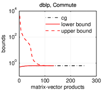
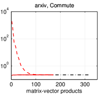
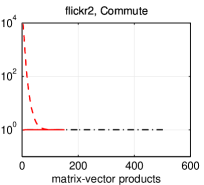
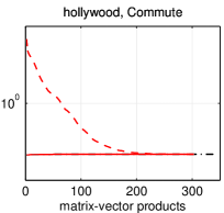
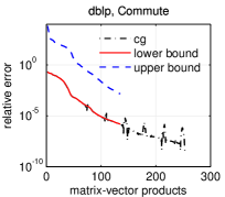
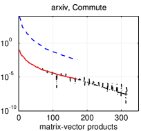
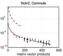
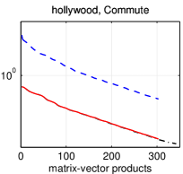
Figure 1: Convergence results for pairwise commute times. (Top row) Each figure shows the upper and lower bounds at each iteration of Algorithm 4 for the graphs dblp, arxiv, flickr2, and hollywood-2009. (Bottom row) For the same graphs, each figure shows the relative size of the error, $(v_{\text{alg}}-v_{\text{exact}})/v_{\text{exact}}$ in the upper and lower bounds at each iteration. In both cases, we also show the same data from the conjugate gradient algorithm. See Section 6.2 for our discussion.

In the figure, the upper bounds and lower bounds “trap” the solution from above and below. These bounds converge smoothly to the final solution. For these experiments, the lower bound has smaller error, and also, this error tracks the performance of CG quite closely. This behavior is expected in cases where the largest eigenvalue of the matrix is well-separated from the remaining eigenvalues – a fact that holds for the Laplacians of our graphs, see Mihail and Papadimitriou (2002) and Chung et al. (2003) for some theoretical justification. When this happens, the Lanczos procedure underlying both our technique and CG quickly produces an accurate estimate of the true largest eigenvalue, which in turn eliminates any effect due to our initial overestimate of the largest eigenvalue. (Recall from Algorithm 4 that the estimate of $\overline{\lambda}$ is present in the computation of the lower-bound $\underline{b_{j}}$.)

Here, the conjugate gradient method suffers two problems. First, because it does not provide bounds on the score, it is not possible to terminate it until the residual is small. Thus, the conjugate gradient method requires more iterations than our pairwise algorithm. Note, however, this result is simply a matter of detecting when to stop – both conjugate gradient and our lower-bound produce similar relative errors for the same work. Second, the relative error for conjugate gradient displays erratic behavior. Such behavior is not unexpected because conjugate gradient optimizes the $A$-norm of the solution error and it is not guaranteed to provide smooth convergence in true error norm. These oscillations make early termination of the CG algorithm problematic, whereas no such issues occur for the upper and lower bounds from our algorithm. We speculate that the seemingly smooth convergence behavior that we observe for the upper and lower bound estimates may be rooted in the convergence behavior of the largest Ritz value of the tridiagonal matrix associated with Lanczos, but a better understanding of this issue will require further exploration.

6.3 Pairwise Katz scores

We next show the same type of figure but for the pairwise Katz scores instead; see Figure 2. We use a value of $\alpha$ that makes $\boldsymbol{I}-\alpha\boldsymbol{A}$ nearly indefinite. Such a value produces the slowest convergence in our experience. The particular value we use is $\alpha=1/(\|\boldsymbol{A}\|_{2}+1)$, which we call “hard alpha” in some of the figure titles. For all of the graphs, we again used $\underline{\lambda}=10^{-4}$ and $\overline{\lambda}={\|\boldsymbol{\tilde{L}}\|}_{1}$. This value of $\underline{\lambda}$ is smaller than the smallest eigenvalue of $\boldsymbol{I}-\alpha\boldsymbol{A}$ for all the graphs. Also, the vertex pairs are the same as those used for Figure 1. For pairwise Katz scores, the baseline approach involves solving the linear system $(\boldsymbol{I}-\alpha\boldsymbol{A})\boldsymbol{\mathrm{x}}=\boldsymbol{\mathrm{e}}_{j}$, again using the conjugate gradient method (CG). At each step of CG, we use the approximation $\boldsymbol{\mathrm{e}}_{i}^{T}\boldsymbol{\mathrm{x}}^{(k)}$, where $\boldsymbol{\mathrm{x}}^{(k)}$ is the $k$h iterate. We use the same convergence check as in the CG baseline for commute time. For these problems, we also evaluated techniques based on the Neumann series for $\boldsymbol{I}-\alpha\boldsymbol{A}$, but those took over 100 times as many iterations as CG or our pairwise approach. The Neumann series is the same algorithm used in Wang et al. (2007) but customized for the linear system, not matrix inverse, which is a more appropriate comparison for the pairwise case. Finally, the exact solution was again computed by using MINRES Paige and Saunders (1975) to solve the same system as CG to a tolerance of $10^{-14}$.

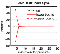
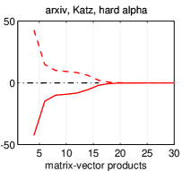
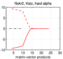
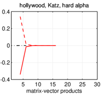
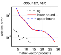
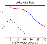
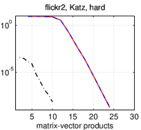
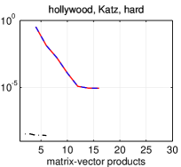
Figure 2: Convergence results for pairwise Katz scores. (Top row.) Each figure shows the upper and lower bounds at each iteration of Algorithm 5 for the graphs dblp, arxiv, flickr2, and hollywood-2009. (Bottom row.) For the same graphs, each figure shows the relative size of the error, $(v_{\text{alg}}-v_{\text{exact}})/v_{\text{exact}}$ in the upper and lower bounds at each iteration. In both cases, we also show the same data from the conjugate gradient algorithm. See Section 6.3 for discussion.

A distinct difference from the commute-time results is that both the lower and upper bounds converge similarly and have similar error. This occurs because of the symmetry in the upper and lower bounds that results from using the MMQ algorithm twice on the form: $(1/4)[(\boldsymbol{\mathrm{e}}_{i}+\boldsymbol{\mathrm{e}}_{j})^{T}(\boldsymbol{I}-\alpha\boldsymbol{A})^{-1}(\boldsymbol{\mathrm{e}}_{i}+\boldsymbol{\mathrm{e}}_{j})-(\boldsymbol{\mathrm{e}}_{i}-\boldsymbol{\mathrm{e}}_{j})^{T}(\boldsymbol{I}-\alpha\boldsymbol{A})^{-1}(\boldsymbol{\mathrm{e}}_{i}-\boldsymbol{\mathrm{e}}_{j})].$ In comparison with the conjugate gradient method, our pairwise algorithm is slower to converge. While the conjugate gradient method appears to outperform our pairwise algorithms here, recall that it does not provide any approximation guarantees. Also, the two matrix-vector product in Algorithm 5 can easily be merged into a single “combined” matrix-vector product algorithm. As we discuss further in the conclusion, such an implementation would reduce the difference in runtime between the two methods.

6.4 Relative matrix-vector products in pairwise algorithms

Thus far, we have detailed a few experiments describing how the pairwise algorithms converge. In these cases, we compared against the conjugate gradient algorithm for a single pair of vertices on each graph. In this experiment, we examine the number of matrix-vector products that each algorithm requires for a much larger set of vertex pairs. Let us first describe how we picked the vertices for the pairwise comparison. There were two types of vertex pairs chosen: purely random, and degree-correlated. The purely random choices are simple: pick a random permutation of the vertex numbers, then use pairs of vertices from this ordering. The degree correlated pairs were picked by first sorting the vertices by degree in decreasing order, then picking the 1st, 2nd, 3rd, 4th, 5th, 10th, 20th, 30th, 40th, 50th, 100th,…vertices from this ordering, and finally, use all vertex pairs in this subset. Note that for commute time, we only used the 1st, 5th, 10th, 50th, 100th,…. vertices to reduce the total computation time. For the pairwise commute times, we used 20 random pairs. and used 100 random pairs for pairwise Katz scores.

In Figure 3, we show the matrix-vector performance ratio between our pair-wise algorithms and conjugate gradient. Let $k_{\text{cg}}$ be the number of matrix-vector products until CG converges to a tolerance of $10^{-4}$ (as in previous experiments); and let $k_{\text{alg}}$ be the number of matrix-vector products until our algorithm converges. The performance ratio is

$$\frac{k_{\text{cg}}-k_{\text{alg}}}{k_{\text{cg}}},$$

which has a value of $0$ when the two algorithms take the same number of matrix-vector products, the value 1 when our algorithm takes 0 matrix-vector products, and the value -1 (or -2) when our algorithm takes twice (or thrice) as many matrix-vector products as CG. We display the results as a box-plot of the results from all trials. There was no systematic difference in the results between the two types of vertex pairs (random or degree correlated).

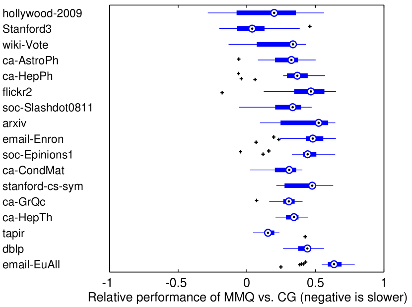
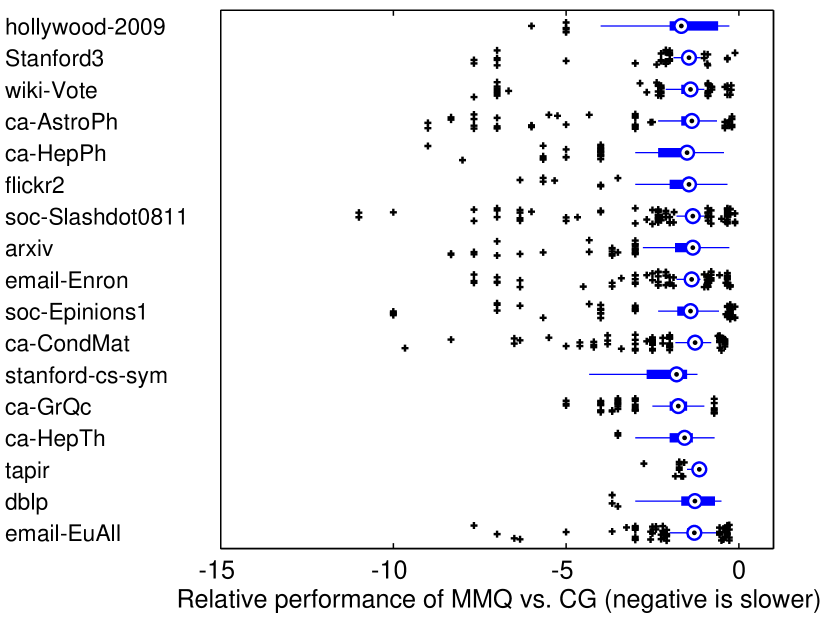
Figure 3: (Left) Relative performance between Algorithm 4 and conjugate gradient for pairwise commute times. (Right) Relative performance between Algorithm 5 and conjugate gradient for pairwise Katz scores. The relative performance measure is $(k_{\text{cg}}-k_{\text{alg}})/k_{\text{cg}}$, where $k$ is the number of matrix-vector products taken by each approach.

These results show that the small sample in the previous section is fairly representative of the overall performance difference. In general, our commute time algorithm uses fewer matrix-vector products than conjugate gradient. We suspect this result is due to the ability to stop early as explained in Section 6.2. And, as also observed in Section 6.3, our pairwise Katz algorithm tends to take 2-3 times as many matrix vector products as conjugate gradient. These results again used the same “hard alpha” value.

6.5 Column-wise commute times

Our next set of results concerns the precision of our approximation to the column-wise commute time scores. Because the output of our column-wise commute time algorithm is based on a coarse approximation of the diagonal elements of the inverse, we do not expect these scores to converge to their exact values as we increase the work in the algorithm. Consequently, we study the results in terms of the precision at $k$missing measure. Recall that the motivation for studying these column-wise measures is not to get the column scores precisely correct, but rather to identify the closest nodes to a given query or target node. That is, we are most interested in the smallest elements of a column of the commute time matrix. Given a target node $i$, let $S_{k}^{\text{alg}}$ be the $k$ closest nodes to $i$ in terms of our algorithm. Also, let $S_{k}^{*}$ be the $k$ closest nodes to $i$ in terms of the exact commute time. (See below for how we compute this set.) The precision at $k$ measure is

$$|S_{k}^{*}\cap S_{k}^{\text{alg}}|/k.$$

In words, this formula computes the fraction of the true set of $k$ nodes that our algorithm identifies.

We ran the algorithm from Section 5.1 with a tolerance of $10^{-16}$ to evaluate the maximum accuracy possible with this approach. We choose 50 target nodes randomly and also based on the same degree sequence sampling mentioned in the last section. For values of $k$ between 5 and 100, we show a box-plot of the precision at $k$ scores for four networks in Figure 4. In the same figure, we also show the result of using the heuristic $C_{i,j}\approx\frac{1}{D_{i,i}}+\frac{1}{D_{j,j}}$ suggested by von Luxburg et al. (2010). This heuristic is called “inverse degree” in the figure, because it shows that the set $S_{k}^{*}$ should look like the set of $k$ nodes with highest degree or smallest inverse degree.

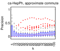
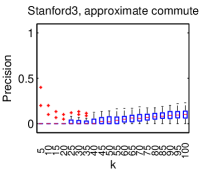
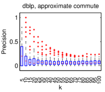
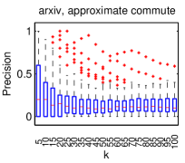
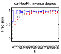
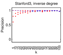
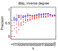
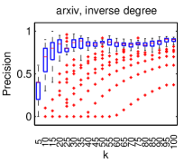
Figure 4: Precision at $k$ for the column-wise commute time approximations (top) over a few hundred trial columns. Precision at $k$ for the inverse degree heuristic (bottom) over the same columns. These figures show standard box-plots of the result for each column.

These results show that our approach for estimating a column of the commute time matrix provides only partial information about the true set. However, these experiments reinforce the theoretical discussion in von Luxburg et al. (2010) that commute time provides little information beyond the degree distribution. Consequently, the results from our algorithm may provide more useful information in practice. Although such a conclusion would require us to formalize the nature of the approximation error in this algorithm, and involve a rather different kind of study.

Exact commute times

Computing commute times is challenging. As part of a separate project, the third author of this paper wrote a program to compute the exact eigenvalue decomposition of a combinatorial graph Laplacian in a distributed computing environment using the MPI and the ScaLAPACK library Blackford et al. (1996). This program ignores the sparsity in the matrix and treats the problem as a dense matrix. We adapted this software to compute the pseudo-inverse of the graph Laplacian as well as the commute times. We were able to run this code on graphs up to 100,000 nodes using approximately 10-20 nodes of a larger supercomputer. (The details varied by graph, and are not relevant for this paper.) For graphs with less than 20,000 nodes, the same program will compute all commute-times on the previously mentioned desktop computer. Thus, we computed the exact commute times for all graphs except email-euAll, flickr2, and hollywood-2009.

6.6 Column-wise Katz scores

We now come to evaluate the local algorithm for Katz scores. As with the pairwise algorithms, we first study the empirical convergence of the algorithm. However, the evaluation for the convergence here is rather different. Recall, again, that the point of the column-wise algorithms is to find the most closely related nodes. For Katz scores, these are the largest elements in a column (whereas for commute time, they were the smallest elements in the column). Thus, we again evaluate each algorithm in terms of the precision at $k$ for the top-$k$ set generated by our algorithms and the exact top-$k$ set produced by solving the linear system. Natural alternatives are other iterative methods and specialized direct methods that exploit sparsity. The latter – including approaches such as truncated commute time Sarkar and Moore (2007) – are beyond the scope of this work, since they require a different computational treatment in terms of caching and parallelization. Thus, we again use conjugate gradient (CG) as our point of comparison. The exact solution is computed by solving $(\boldsymbol{I}-\alpha\boldsymbol{A})\boldsymbol{\mathrm{k}}_{i}=\boldsymbol{\mathrm{e}}_{i}$, again using the MINRES method, to a tolerance of $10^{-12}$.

We also look at the Kendall-$\tau$ correlation coefficient between our algorithm’s results and the exact top-$k$ set. This experiment will let us evaluate whether the algorithm is ordering the true set of top-$k$ results correctly. Let $x_{k^{\ast}}^{\text{alg}}$ be the scores from our algorithm on the exact top-$k$ set, and let $x_{k^{\ast}}^{\ast}$ be the true top-$k$ scores. The $\tau$ coefficients are computed between $x_{k^{\ast}}^{\text{alg}}$ and $x_{k^{\ast}}^{\ast}$.

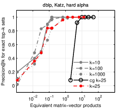
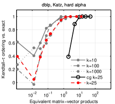
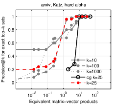
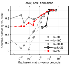
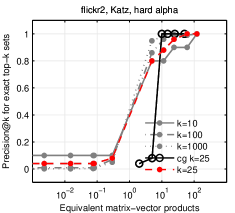
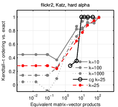
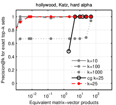
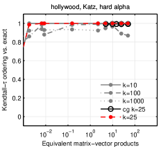
Figure 5: Convergence results for our column-wise Katz algorithm in terms of the precision of the top-$k$ set (left) and the ordering of the true top-$k$ set (right). See Section 6.6 for the discussion.

Both of the precision at $k$ and the Kendall-$\tau$ measures should tend to $1$ as we increase the work in our algorithm. Indeed, this is what we observe in Figure 5. For these figures, we pick a vertex with a fairly large degree and run Algorithm 6 with the “hard alpha” value mentioned in previous sections. As the algorithm runs, we track work with respect to the number of effective matrix vector products. An effective matrix-vector product corresponds to our algorithm examining the same number of edges as a matrix-vector product. For example, suppose the algorithm accesses a total of $80$ neighbors in a graph with $16$ edges. Then this instance corresponds to $2.5$ effective matrix vector products. The idea is that the amount of work in one effective matrix vector product is about the same as the amount of work in one iteration of CG. Hence, we can compare algorithms on this ground. As evident from the legend in each figure, we look at precision at $k$ for four values of $k$, $10,25,100,1000$, and also the Kendall-$\tau$ for these same values. While all of the measures should tend to 1 as we increase work, some of the exact top-$k$ results contain tied values. Our algorithm has trouble capturing precisely tied values and the effect is that our Kendall-$\tau$ score does not always tend to $1$ exactly.

For comparison, we show results from the conjugate gradient method for the top-$25$ set after $2,5,10,15,25,$ and $50$ matrix-vector products. In these results, the top-$25$ set is nearly converged after the equivalent of a single matrix-vector product – equivalent to just one iteration of the CG algorithm. The CG algorithm does not provide any useful information until it converges. Our top-$k$ algorithm produces useful partial information in much less work.

6.7 Runtime

Finally, we show the empirical runtime of our implementations in Tables 4 and 5. Table 4 describes the runtime of the two pairwise algorithms. We show the 25th, 50th, and 75th percentiles of the time taken to compute the results from Figure 3. Our implementation is not optimized, and so these results indicate the current real-world performance of the algorithms.

Table 5 describes the runtime of the column-wise Katz algorithm. Here, we picked columns of the matrix to approximate in two ways: (i) randomly, and (ii) to sample the entire degree distribution. As in previous experiments, we took the 1st, 2nd, 3rd, 4th, 5th, 10th, 20th,…vertices from the set of vertices sorted in order of decreasing degree. For each column picked in this manner, we ran Algorithm 6 and recorded the wall clock time. The 25th, 50th, and 75th percentiles of these times are shown in the table for each of the two sets of vertices.

For this algorithm, the degree of the target node has a considerable impact on the algorithm runtime. This effect is particularly evident in the flick2 data. The randomly chosen columns are found almost instantly, whereas the degree sampled columns take considerably longer. A potential explanation for this behavior is that starting at a vertex with a large degree will dramatically increase the residual at the first step. If these new vertices also have a large degree, then this effect will multiply and the residual will rise for a long time before converging. Even in the cases where the algorithm took a long time to converge, it only explored a small fraction of the graph (usually about 10% of the vertices), and so it retained its locality property. This property suggests that optimizing our implementation could reduce these runtimes.

Table 4: Runtime of the pair-wise algorithms. The “0.0” second entries are rounded down for display. These are really just less than 0.1 seconds. The three columns for each type of problem show the 25th, 50th, and 75th percentiles of the wall-clock time to compute the results in Figure 3.

Graph	Verts.	Avg.	Pair-wise Katz			Pair-wise commute
		Deg.	runtime (sec.)			runtime (sec.)
			25%	Median	75%	25%	Median	75%
tapir	1024	5.6	0.0	0.0	0.0	0.0	0.0	0.1
stanford-cs	2759	7.4	0.0	0.0	0.0	0.1	0.2	0.2
ca-GrQc	4158	6.5	0.0	0.0	0.0	0.1	0.1	0.1
wiki-Vote	7066	28.5	0.0	0.0	0.0	0.2	0.2	0.2
ca-HepTh	8638	5.7	0.0	0.0	0.0	0.1	0.2	0.2
ca-HepPh	11204	21.0	0.0	0.0	0.0	0.4	0.4	0.4
Stanford3	11586	98.1	0.2	0.2	0.2	0.6	0.7	0.7
ca-AstroPh	17903	22.0	0.1	0.1	0.1	0.5	0.5	0.7
ca-CondMat	21363	8.5	0.0	0.0	0.1	0.4	0.5	0.5
email-Enron	33696	10.7	0.1	0.1	0.1	1.1	1.2	1.3
soc-Epinions1	75877	10.7	0.2	0.2	0.2	2.8	3.2	3.7
soc-Slashdot0811	77360	12.1	0.2	0.2	0.2	2.6	2.8	3.4
arxiv	86376	12.0	0.2	0.3	0.3	4.8	6.0	6.5
dblp	93156	3.8	0.1	0.1	0.2	3.0	3.2	3.4
email-EuAll	224832	3.0	0.3	0.4	0.4	11.2	14.2	17.2
flickr2	513969	12.4	1.3	1.7	1.8	54.8	60.0	69.8
hollywood-2009	1069126	105.3	16.5	17.0	17.4	199.2	246.0	272.5

Table 5: Runtime of the column-wise Katz algorithm. The “0.0” second entries are rounded down for display. These are really just less than 0.1 seconds. The three columns show the 25th, 50th, and 75th percentiles of the wall-clock time of the experiments described in Section 6.7.

Graph	Verts.	Avg.	Random columns			Degree columns
		Deg.	runtime (sec.)			runtime (sec.)
			25%	Median	75%	25%	Median	75%
tapir	1024	5.6	0.0	0.0	0.0	0.0	0.0	0.0
stanford-cs-sym	2759	7.4	0.0	0.0	0.0	0.0	0.0	0.0
ca-GrQc	4158	6.5	0.0	0.0	0.0	0.0	0.0	0.0
wiki-Vote	7066	28.5	0.0	0.0	0.4	0.4	0.4	0.4
ca-HepTh	8638	5.7	0.0	0.0	0.0	0.0	0.0	0.0
ca-HepPh	11204	21.0	0.0	0.0	0.0	1.1	1.1	1.1
Stanford3	11586	98.1	0.0	0.0	1.7	1.8	1.9	1.9
ca-AstroPh	17903	22.0	0.0	0.0	0.0	0.6	0.7	0.9
ca-CondMat	21363	8.5	0.0	0.0	0.0	0.1	0.1	0.1
email-Enron	33696	10.7	0.0	0.0	0.0	0.9	1.0	1.1
soc-Epinions1	75877	10.7	0.0	0.0	0.0	3.7	4.1	4.5
soc-Slashdot0811	77360	12.1	0.0	0.0	0.0	2.4	2.8	3.7
arxiv	86376	12.0	0.0	0.0	0.0	0.0	0.6	0.7
dblp	93156	3.8	0.0	0.0	0.0	0.0	0.0	0.0
email-EuAll	224832	3.0	0.0	0.0	0.0	1.1	1.7	2.5
flickr2	513969	12.4	0.0	0.0	0.0	11.5	52.6	55.5
hollywood-2009	1069126	105.3	0.0	0.0	0.0	0.3	0.4	0.4

7 Conclusion and Discussion

The goal of this manuscript is to estimate commute times and Katz scores in a rapid fashion. Let us summarize our contributions and experimental findings.

• For the pair-wise commute time problem, we have implemented Algorithm 4, based on the relationship between the Lanczos process and a quadrature rule (Section 4.1). This algorithm uses a similar mechanism to that of conjugate gradient (CG). It outperforms the latter in terms of total matrix-vector products, because it provides upper and lower bounds that allow for early termination, whereas CG does not provide an easy way of detecting convergence for a specific pairwise score.

• For the pair-wize Katz problem, we have proposed Algorithm 5, also based on the same quadrature theory. This algorithm involves two simultaneous Lanczos iterations. In practice, this means more work per iteration than a simple approach based on CG. A careful implementation of Algorithm 5 would merge the two Lanczos processes into a “joint process” and perform the matrix-vector products simultaneously. In our tests of this idea, we have found that the combined matrix-vector product took only 1.5 times as long as a single matrix-vector product.

• For the column-wise commute time problem, we have investigated a variation of the conjugate gradient method that also provides an estimate of the diagonals of the matrix inverse. We have found that these estimates were fairly crude approximations of the commute time scores. We have also investigated whether the degree-based heuristic from von Luxburg et al. (2010) provides better information. It indeed seems to perform better, which suggests that the smallest elements of a column of the commute-time matrix may not be a useful set of useful related nodes.

• For the column-wise Katz algorithm, we have proposed Algorithm 6 based on the techniques used for personalized PageRank computing. The idea with these techniques is to exploit sparsity in the solution vector itself to derive faster algorithms. We have shown that this algorithm converged in two cases: Remark 1, where we established a precise convergence result, and Theorem 3, where we only established asymptotic convergence.

We believe that these results paint a useful picture of the strengths and limitations of our algorithms. Here are a few possible directions for future work:

Alternatives for pair-wise Katz.

First, there are alternatives to using the identity $\boldsymbol{\mathrm{u}}^{T}f(\boldsymbol{Z})\boldsymbol{\mathrm{v}}=(1/4)(\boldsymbol{\mathrm{u}}+\boldsymbol{\mathrm{v}})^{T}f(\boldsymbol{Z})(\boldsymbol{\mathrm{u}}+\boldsymbol{\mathrm{v}})-(1/4)(\boldsymbol{\mathrm{u}}-\boldsymbol{\mathrm{v}})^{T}f(\boldsymbol{Z})(\boldsymbol{\mathrm{u}}-\boldsymbol{\mathrm{v}})$ in the $\boldsymbol{\mathrm{u}}\not=\boldsymbol{\mathrm{v}}$ case. The first alternative is based on the nonsymmetric Lanczos process Golub and Meurant (2010). This approach still requires two matrix-vector products per iteration, but it directly estimates the bilinear form and also provides upper and lower bounds. A concern with the nonsymmetric Lanczos process is that it is possible to encounter degeneracies in the recurrence relationships that stop the process short of convergence. Another alternative is based on the block Lanczos process Golub and Meurant (2010). However, this process does not yet offer upper and lower bounds.

A theoretical basis for the localization of Katz scores.

The inspiration for the column-wise Katz algorithm were the highly successful personalized PageRank algorithms. The localization of these personalized PageRank vectors was made precise in a theorem from Andersen et al. (2006) that related the personalized PageRank vector to cuts in the graph. In brief, if there is a good cut nearby a vertex, then the personalized PageRank vector will be localized on a few vertices. An interesting question is whether or not Katz matrices enjoy a similar property. We hope to investigate this question in the future.

References

- Acar et al. [2009] Evrim Acar, Daniel M. Dunlavy, and Tamara G. Kolda. Link prediction on evolving data using matrix and tensor factorizations. In ICDMW ’09: Proceedings of the 2009 IEEE International Conference on Data Mining Workshops, pages 262–269. IEEE Computer Society, 2009. ISBN 978-0-7695-3902-7. doi: 10.1109/ICDMW.2009.54.
- Andersen et al. [2006] Reid Andersen, Fan Chung, and Kevin Lang. Local graph partitioning using PageRank vectors. In Proc. of the 47th Annual IEEE Sym. on Found. of Comp. Sci., 2006. URL http://www.math.ucsd.edu/~fan/wp/localpartition.pdf.
- Benzi and Boito [2010] Michele Benzi and Paola Boito. Quadrature rule-based bounds for functions of adjacency matrices. Linear Algebra and its Applications, 433(3):637–652, 2010.
- Berkhin [2007] Pavel Berkhin. Bookmark-coloring algorithm for personalized PageRank computing. Internet Math., 3(1):41–62, 2007. URL http://www.internetmathematics.org/volumes/3/1/Berkhin.pdf.
- Blackford et al. [1996] Laura Susan Blackford, J. Choi, A. Cleary, A. Petitet, R. C. Whaley, J. Demmel, I. Dhillon, K. Stanley, J. Dongarra, S. Hammarling, G. Henry, and D. Walker. Scalapack: a portable linear algebra library for distributed memory computers - design issues and performance. In Proceedings of the 1996 ACM/IEEE conference on Supercomputing (CDROM), Supercomputing ’96, Washington, DC, USA, 1996. IEEE Computer Society. ISBN 0-89791-854-1. doi: 10.1145/369028.369038.
- Boldi and Vigna [2004] Paolo Boldi and Sebastiano Vigna. The Webgraph Framework I: Compression techniques. In Proceedings of the 13th international conference on the World Wide Web, pages 595–602, New York, NY, USA, 2004. ACM Press. ISBN 1-58113-844-X. doi: 10.1145/988672.988752.
- Boldi et al. [2011] Paolo Boldi, Marco Rosa, Massimo Santini, and Sebastiano Vigna. Layered label propagation: A multiresolution coordinate-free ordering for compressing social networks. In Proceedings of the 20th WWW2011, pages 587–596, March 2011.
- Chantas et al. [2008] G. Chantas, N. Galatsanos, A. Likas, and M. Saunders. Variational bayesian image restoration based on a product of -distributions image prior. Image Processing, IEEE Transactions on, 17(10):1795–1805, October 2008. ISSN 1057-7149. doi: 10.1109/TIP.2008.2002828.
- Chung et al. [2003] Fan Chung, Linyuan Lu, and Van Vu. Eigenvalues of random power law graphs. Annals of Combinatorics, 7(1):21–33, 2003. URL http://www.springerlink.com/content/0wjwr2jd0bg9lmqy/.
- Davis and Rabinowitz [1984] P. J. Davis and P. Rabinowitz. Methods of Numerical Integration. Academic Press, New York, 2nd edition, 1984.
- Davis and Hu [2010] Timothy A. Davis and Yifan Hu. The university of florida sparse matrix collection. ACM Transactions on Mathematical Software, 2010. URL http://www.cise.ufl.edu/research/sparse/matrices/. To appear.
- Farkas et al. [2001] Illés J. Farkas, Imre Derényi, Albert-László Barabási, and Tamás Vicsek. Spectra of “real-world” graphs: Beyond the semicircle law. Phys. Rev. E, 64(2):026704, July 2001. doi: 10.1103/PhysRevE.64.026704.
- Foster et al. [2001] Kurt C. Foster, Stephen Q. Muth, John J. Potterat, and Richard B. Rothenberg. A faster Katz status score algorithm. Comput. & Math. Organ. Theo., 7(4):275–285, 2001.
- Fouss et al. [2007] François Fouss, Alain Pirotte, Jean-Michel Renders, and Marco Saerens. Random-walk computation of similarities between nodes of a graph with application to collaborative recommendation. IEEE Trans. Knowl. Data Eng., 19(3):355–369, 2007.
- Gilbert and Teng [2002] John R. Gilbert and Shang-Hua Teng. MESHPART: Matlab mesh partitioning and graph separator toolbox. http://www.cerfacs.fr/algor/Softs/MESHPART/, February 2002. URL http://www.cerfacs.fr/algor/Softs/MESHPART/.
- Göbel and Jagers [1974] F. Göbel and A. A. Jagers. Random walks on graphs. Stochastic Processes and their Applications, 2(4):311–336, 1974. ISSN 0304-4149. doi: 10.1016/0304-4149(74)90001-5. URL http://www.sciencedirect.com/science/article/B6V1B-45FCH5T-Y/2/6a06d2db0d543df84aced9e88a125176.
- Golub and Meurant [1994] G. H. Golub and Gérard Meurant. Matrices, moments and quadrature. In Numerical analysis 1993 (Dundee, 1993), volume 303 of Pitman Res. Notes Math. Ser., pages 105–156. Longman Sci. Tech., Harlow, 1994.
- Golub and Meurant [1997] Gene H. Golub and Gérard Meurant. Matrices, moments and quadrature ii; how to compute the norm of the error in iterative methods. BIT Num. Math., 37(3):687–705, 1997.
- Golub and Meurant [2010] Gene H. Golub and Gérard Meurant. Matrices, Moments, and Quadrature with Applications. Princeton Series in Applied Mathematics. Princeton University Press, 2010.
- Hirai et al. [2000] Jun Hirai, Sriram Raghavan, Hector Garcia-Molina, and Andreas Paepcke. Webbase: a repository of web pages. Computer Networks, 33(1-6):277–293, June 2000. doi: 10.1016/S1389-1286(00)00063-3.
- Jeh and Widom [2002] Glen Jeh and Jennifer Widom. Simrank: a measure of structural-context similarity. In Proc. of the 8th ACM Intl. Conf. on Know. Discov. and Data Mining (KDD’02), 2002.
- Katz [1953] Leo Katz. A new status index derived from sociometric analysis. Psychometrika, 18:39–43, 1953.
- Lanczos [1950] Cornelius Lanczos. An iteration method for the solution of the eigenvalue problem of linear differential and integral operators. Journal of Research of the National Bureau of Standards, 45(4):255–282, October 1950. URL http://nvl.nist.gov/pub/nistpubs/jres/045/4/V45.N04.A01.pdf.
- Lanczos [1952] Cornelius Lanczos. Solution of systems of linear equations by minimized iterations. Journal of Research of the National Bureau of Standards, 49(1):33–53, July 1952. URL http://nvl.nist.gov/pub/nistpubs/jres/049/1/V49.N01.A06.pdf. Research paper 2341.
- Lehoucq et al. [1997] R. B. Lehoucq, D. C. Sorensen, and C. Yang. ARPACK User’s Guide: Solution of Large Scale Eigenvalue Problems by Implicitly Restarted Arnoldi Methods, October 1997. URL http://www.caam.rice.edu/software/ARPACK/SRC/ug.ps.gz.
- Leskovec [2010] Jure Leskovec. The stanford large network dataset collection. http://snap.stanford.edu/data/index.html, 2010.
- Leskovec et al. [2007] Jure Leskovec, Jon Kleinberg, and Christos Faloutsos. Graph evolution: Densification and shrinking diameters. ACM Trans. Knowl. Discov. Data, 1:1–41, March 2007. ISSN 1556-4681. doi: 10.1145/1217299.1217301.
- Leskovec et al. [2009] Jure Leskovec, Kevin J. Lang, Anirban Dasgupta, and Michael W. Mahoney. Community structure in large networks: Natural cluster sizes and the absence of large well-defined clusters. Internet Mathematics, 6(1):29–123, September 2009. doi: 10.1080/15427951.2009.10129177.
- Leskovec et al. [2010] Jure Leskovec, Daniel Huttenlocher, and Jon Kleinberg. Signed networks in social media. In Proceedings of the 28th international conference on Human factors in computing systems, CHI ’10, pages 1361–1370, New York, NY, USA, 2010. ACM. ISBN 978-1-60558-929-9. doi: 10.1145/1753326.1753532.
- Li et al. [2010] Pei Li, Hongyan Liu, Jeffrey Xu Yu, Jun He, and Xiaoyong Du. Fast single-pair simrank computation. In Proc. of the SIAM Intl. Conf. on Data Mining (SDM2010), Columbus, OH, 2010.
- Liben-Nowell and Kleinberg [2003] David Liben-Nowell and Jon M. Kleinberg. The link prediction problem for social networks. In Proc. of the ACM Intl. Conf. on Inform. and Knowlg. Manage. (CIKM’03), 2003.
- Luo and Tseng [1992] Z. Q. Luo and P. Tseng. On the convergence of the coordinate descent method for convex differentiable minimization. Journal of Optimization Theory and Applications, 72(1):7–35, 1992. ISSN 0022-3239. doi: 10.1007/BF00939948. 10.1007/BF00939948.
- McSherry [2005] Frank McSherry. A uniform approach to accelerated PageRank computation. In Proc. of the 14th Intl. Conf. on the WWW, pages 575–582, New York, NY, USA, 2005. ACM Press. ISBN 1-59593-046-9. doi: 10.1145/1060745.1060829.
- Mihail and Papadimitriou [2002] Milena Mihail and Christos H. Papadimitriou. On the eigenvalue power law. In RANDOM ’02: Proceedings of the 6th International Workshop on Randomization and Approximation Techniques, pages 254–262, London, UK, 2002. Springer-Verlag. ISBN 3-540-44147-6. doi: 10.1007/3-540-45726-7˙20.
- O’Leary [1980] Dianne P. O’Leary. The block conjugate gradient algorithm and related methods. Linear Algebra and its Applications, 29:293 – 322, 1980. ISSN 0024-3795. doi: 10.1016/0024-3795(80)90247-5. URL http://www.sciencedirect.com/science/article/B6V0R-45GWM37-T/2/61817ca45178e6911a3d537c05b4b1fb.
- Page et al. [1999] Lawrence Page, Sergey Brin, Rajeev Motwani, and Terry Winograd. The PageRank citation ranking: Bringing order to the web. Technical Report 1999-66, Stanford University, November 1999. URL http://dbpubs.stanford.edu:8090/pub/1999-66.
- Paige and Saunders [1975] C. C. Paige and M. A. Saunders. Solution of sparse indefinite systems of linear equations. SIAM Journal on Numerical Analysis, 12(4):617–629, 1975. doi: 10.1137/0712047. URL http://link.aip.org/link/?SNA/12/617/1.
- Rattigan and Jensen [2005] Matthew J. Rattigan and David Jensen. The case for anomalous link discovery. SIGKDD Explor. Newsl., 7(2):41–47, 2005.
- Richardson et al. [2003] Matthew Richardson, Rakesh Agrawal, and Pedro Domingos. Trust management for the semantic web. In The SemanticWeb - ISWC 2003, volume 2870 of Lecture Notes in Computer Science, pages 351–368. Springer Berlin / Heidelberg, 2003. doi: 10.1007/978-3-540-39718-2˙23.
- Saerens et al. [2004] Marco Saerens, François Fouss, Luh Yen, and Pierre Dupont. The principal components analysis of a graph, and its relationships to spectral clustering. In Proc. of the 15th Euro. Conf. on Mach. Learn., 2004.
- Sarkar and Moore [2007] Purnamrita Sarkar and Andrew W. Moore. A tractable approach to finding closest truncated-commute-time neighbors in large graphs. In Proc. of the 23rd Conf. on Uncert. in Art. Intell. (UAI’07), 2007.
- Sarkar et al. [2008] Purnamrita Sarkar, Andrew W. Moore, and Amit Prakash. Fast incremental proximity search in large graphs. In Proc. of the 25th Intl. Conf. on Mach. Learn. (ICML’08), 2008.
- Saunders [2007] Michael Saunders. cgLanczos: CG method for positive definite ax=b. http://www.stanford.edu/group/SOL/software/cgLanczos.html, accessed on 2011-03-25, 2007.
- Spielman and Srivastava [2008] Daniel A. Spielman and Nikhil Srivastava. Graph sparsification by effective resistances. In Proc. of the 40th Ann. ACM Symp. on Theo. of Comput. (STOC’08), pages 563–568, 2008.
- Traud et al. [2011] Amanda L. Traud, Peter J. Mucha, and Mason A. Porter. Social structure of facebook networks. arXiv, cs.SI:1102.2166, February 2011. URL http://arxiv.org/abs/1102.2166.
- Varga [1962] R.S. Varga. Matrix Iterative Analysis. Prentice-Hall, 1962.
- von Luxburg et al. [2010] Ulrike von Luxburg, Agnes Radl, and Matthias Hein. Getting lost in space: Large sample analysis of the commute distance. In Advances in Neural Information Processing Systems 24 (NIPS2010), 2010. URL http://books.nips.cc/papers/files/nips23/NIPS2010_0929.pdf.
- Wang et al. [2007] Chao Wang, Venu Satuluri, and Srinivasan Parthasarathy. Local probabilistic models for link prediction. In ICDM ’07: Proceedings of the 2007 Seventh IEEE International Conference on Data Mining, pages 322–331, Washington, DC, USA, December 2007. IEEE Computer Society. ISBN 0-7695-3018-4. doi: 10.1109/ICDM.2007.108.
- Yen et al. [2007] L. Yen, F. Fouss, C. Decaestecker, P. Francq, and M. Saerens. Graph nodes clustering based on the commute-time kernel. In Proc. of the 11th Pacific-Asia Conf. on Knowled. Disc. and Data Mining (PAKDD 2007). Lecture Notes in Computer Science (LNCS), 2007.