Magnetic measurement with coils and wires

Abstract

Accelerator magnets steer particle beams according to the field integrated along the trajectory over the magnet length. Purpose-wound coils measure these relevant parameters with high precision and complement efficiently point-like measurements performed with Hall plates or NMR probes. The rotating coil method gives a complete two-dimensional description of the magnetic field in a series of normal and skew multipoles. The more recent single stretched wire is a reference instrument to measure field integrals and to find the magnetic axis.

0.1 Introduction

The field of measurement of accelerator magnets has followed the requirements dictated by developments in accelerator technology. Synchrotron Light Sources require stringent magnetic axis alignment. The field quality of superconducting magnets for an accelerator like the Large Hadron Collider (LHC) has been measured to unprecedented precision, including the time and ramp rate dependent effects due to superconductor cables.

Measuring coils and more recently stretched wires are used extensively for accelerator magnets since they measure the parameters seen by particle beams: magnetic field components in the plane perpendicular to their trajectory and integrated over the length of the magnets. Coils and wires allow fast measurements with data already reduced to the requirements.

This field of physics has benefited from the development in electronic components. Fast acquisition voltmeters or recent 18-bit ADCs with sampling times in the range of microseconds increase the bandwidth and the precision of voltage integrated over time, the basis of this type of measurement.

Section 0.2 describes the classical method of coils flipped by half a turn inside dipole magnets or static coils in pulsed magnets. They are still in use to measure resistive dipoles having flat horizontal aperture and in particular for magnets having a small radius of curvature. In addition, the theory developed for these simple coils must be understood to avoid flaws with more sophisticated measurement methods. Section 0.3 introduces the concept of coil arrays to suppress the contribution from some harmonic components, a concept fundamental to the accurate use of the harmonic coil method.

Sections 0.4 to LABEL:sec:Vibrating group the Single Stretched Wire (SSW) based methods. They measure with high absolute precision the fundamental parameters of accelerator magnets. Section 0.4 introduces the equipment and demonstrates that the SSW gives an absolute value of the field integrated over the magnet length with a minimum of calibration concern. Section 0.5 details how to reference in all dimensions the position of the quadrupole magnet axis and field direction. Section LABEL:sec:sswquadrupole gives the most accurate method to quantify the integrated field gradient and address the issues related to wire deflection due to gravity and magnetic susceptibility. The vibrating wire method described in Section LABEL:sec:Vibrating is still subject to interesting developments in order to find the axis of individual magnets aligned on a girder. It is probably the only candidate method to measure small-aperture magnets under development for high-energy linear accelerators.

Sections LABEL:sec:Harmcoil to LABEL:sec:HarmExperience cover the harmonic or rotating coil method. This technique gives high resolution and measures in one coil revolution all relevant parameters of any accelerator magnet. Both theoretical and experimental developments allow one to confidently design sophisticated instruments measuring with high bandwidth and precision the full harmonic content of a magnet.

0.2 Coils to measure dipole magnets

The following section describes methods that measure only partially the 2D field along the axis of accelerator magnets. The rotating coil method (Section LABEL:sec:Harmcoil and following) gives a complete measurement of any 2D field expressed in a formal way by a series of complex multipoles. It cannot, however, be used in the following cases which are relevant for most ‘accelerator magnets’ compared to storage rings:

• dipole magnets of small accelerators are bent,

• they mostly have wide horizontal apertures compared to the gap height,

• the rotating coil method does not (easily) measure pulsed fields, when $\Delta B/\Delta t$ cannot be neglected over one coil revolution period.

0.2.1 Flip coils for dipole magnet strength

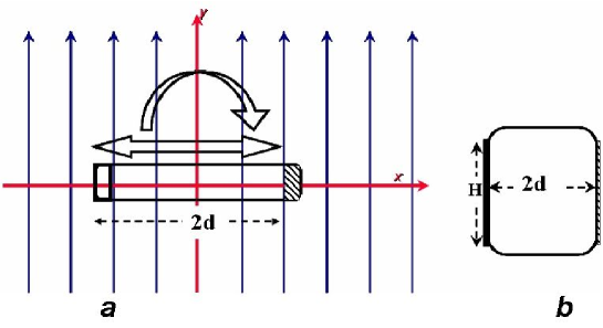
Figure 1: (a) A simple coil, flipped in a dipole field to measure the central field, displaced laterally to measure the field quality. (b) Square coil with a single layer winding insensitive to the sextupole terms when $H=2d$.

The flux picked by the single-turn coil of width $2d$ sketched in fig:flipcoil(a) that is longer than the magnet of length $L$ and that rotates by half a turn is

$$\Psi(\pi)-\Psi(0)=2\cdot\int_{0}^{L}{\int_{-d}^{d}{B_{y}(x)\cdot dx\cdot dl}}\leavevmode\nobreak\ .$$ (1)

By assuming either a perfect dipole, i.e., $B_{y}(x,y)$ constant over the aperture or a coil of width $2d$ small compared to the field errors, i.e., the higher harmonics present in the magnet, the quantities relevant for the particle beam are deduced for the excitation current $I$ in the magnet assumed to be constant during the time to flip the coil:

Dipole strength $$=\left[\int{B_{y}\cdot dl}\right](I)\qquad\text{in\leavevmode\nobreak\ \leavevmode\nobreak\ [T$\cdot$m].}$$ (2)

Transfer function $$=\left[\int{B_{y}\cdot dl}\right](I)/I\qquad\text{in\leavevmode\nobreak\ \leavevmode\nobreak\ [T$\cdot$m{}/{}A].}$$ (3)

The measuring coil has to be longer than the magnet. A rule of thumb says that the coil should extend outside both magnet ends by 2.5 times the aperture. To quantify the validity of this approximation, there is no other way than to perform a $B(z)$ scanning with a Hall plate or to make a full 3D calculation of the stray field in the magnet ends.

0.2.2 Coils displaced horizontally to measure the field quality

The first order imperfections to consider in a resistive magnet are the variation of the vertical field over the aperture width $\Delta B_{y}(x)$. The situation is more complex in superconducting magnets where a non-negligible horizontal field component $B_{x}(x)$ can be present in the horizontal mid-plane. The full 2D complex formalism has then to be applied to describe the field harmonics that can be measured by the rotating coil method covered from sec:Harmcoil onward. An horizontal displacement $\Delta x$ of the coil of fig:flipcoil(a) leads per unit length along the magnet axis to

$$\frac{\Delta B_{y}(x)}{\Delta x}=\frac{\Psi(x+\Delta x)-\Psi(x)}{2d}\leavevmode\nobreak\ .$$ (4)

[b]fig:cnaocurves gives the field quality in the horizontal symmetry plane of 10 dipole magnets for the CNAO facility (sec:CNAO). These curves were measured, for efficiency reasons, in pulsed current mode by 11 different static coils rather than 10 horizontal displacements.

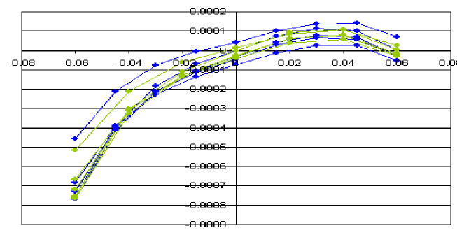
Figure 2: $\Delta B_{y}(x)/\Delta x$ measured on 10 CNAO dipole magnets with the 11-coil fluxmeter

0.2.3 A real coil has finite dimensions for the winding

One way to increase the voltage amplitude at the coil terminals is to increase the width $2d$ therefore picking a vertical field non-constant over this width according to the field quality of the magnet. What is measured is no longer the field at the centre of the coil. The real part of Eq. (LABEL:eq:eqH6) gives

$$B_{y}(x,y)=B_{1}+B_{2}\cdot x+B_{3}\cdot(x^{2}-y2)+...\leavevmode\nobreak\ .$$ (5)

Integrating over the coil width going from $[x-d]$ to $[x+d]$ leads, with the hypothesis of a negligible winding height, to

$$\Psi(x)=B_{1}\cdot 2d+B_{2}\cdot 2dx+B_{3}\cdot(6dx^{2}+2d^{3})+...\leavevmode\nobreak\ .$$ (6)

This equation indicates that a measurement with a half-turn flip is never sensitive to the even harmonics (quadrupole, octupole, etc.) as long as the axis of rotation is centred in the middle of the coil. On the other hand, the sextupole component enters in a dipole strength measurement:

$$\Psi(\pi,x=0)-\Psi(0,x=0)=2.(B_{1}\cdot 2d+B_{3}\cdot 2d^{3})+...\leavevmode\nobreak\ .$$ (7)

All multipole terms enter with different and varying sensitivities when measuring the field quality by a displaced coil:

$$\Psi(x+\delta)-\Psi(x)=B_{2}\cdot 2d\delta+B_{3}\cdot 6d\cdot(2x\delta+\delta^{2})+...\leavevmode\nobreak\ .$$ (8)

Coils with several turns are used to further increase the sensitivity. The winding has then a non-zero cross-section. The coil of fig:flipcoil(b), with coil width equal to the winding height is easily calculated to have no sensitivity to the sextupole $B_{3}$ terms. The issue detailed by Eq. (7) for flip coil measurement is therefore limited to higher orders: starting with the decapole term present in the magnet.

This way of avoiding sensitivity to higher multipole terms was generalized in theory long ago with the fluxball [Brown45]. This fluxball coil, as sketched in fig:fluxball seems difficult to manufacture but picks up a flux equal to the field at the centre of the ball and independent of the spatial harmonics present. A coil approximating this possibility of measuring the field central to a highly sensitive coil probe has been proposed in GreenCAS98.

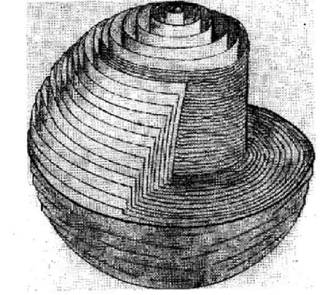
Figure 3: A fluxball, composed of cylindrical windings, measures the field at the central point of the ball

0.2.4 Static coils in pulsed fields

Most accelerator magnets have to be measured in fast current ramping conditions. The coil of fig:flipcoil(b), insensitive in that case to terms lower than the decapole, is an easy tool to use in fixed position in a field pulsed from 0 to nominal value. Modern integrators with large bandwidth and time resolution connected to such a coil can give the full $B_{1}(t)$ curve and measure saturation effects of the iron yoke. Hysteresis and eddy current effects can be separated by measurements at different ramp rates. One precaution deals with the remanent field of the magnet being measured, i.e., the field at zero current value. Three ways can be used to solve it:

• have a bipolar power supply to perform symmetric sweeps from negative to positive maximum current;

• demagnetize the magnet first, with either a bipolar supply or a supply with an inverter;

• measure the remanent field with a flip coil or Hall plates for instance, low accuracy is sufficient in most of the cases.

0.3 Arrays of coils to measure quadrupoles or higher order multipoles

0.3.1 Two-coil array for quadrupole strength and field quality

The measurement of the strength of a quadrupole magnet could be done by the displaced coil method of sec:coils-displaced. High accuracy requires high precision displacement of the coils and the measurement of the field quality, i.e., higher order multipoles, leads to a uselessly complex mathematical treatment. The array of two coils connected in electrical opposition and sketched in fig:quadcoil is often used to give the quadrupole strength by flipping them about their symmetry axis. The coil array, the distance $D$, can be calibrated once in a known quadrupole. The field quality is deduced by displacing, along the $x$ and $y$ axis, the array in a quadrupole in the same way as the the single coil displacement to measure the field quality of a dipole magnet sec:coils-displaced). [b]eq:coilarray1 is valid as long as the two coils have an equal effective surface.

$$B_{1}(x+D)-B_{1}(x-D)=2\cdot D\cdot G(x)\leavevmode\nobreak\ .$$ (9)

The idea of using two coils connected in opposition in order to cancel the contribution of the dipole component is appreciably more effectively used with the rotating coil method (Sections LABEL:sec:dipcomp and LABEL:sec:quadcomp). In that case, the compensation scheme suppresses the main harmonic of the magnet. It is therefore much more powerful for accurate field quality measurements. The rotating coil equipment is more complex to manufacture but is preferred for quadrupole magnets that are straight and have a circular aspect ratio. The present method is, however, mentioned as useful for combined-function magnets and pulsed magnet measurements.

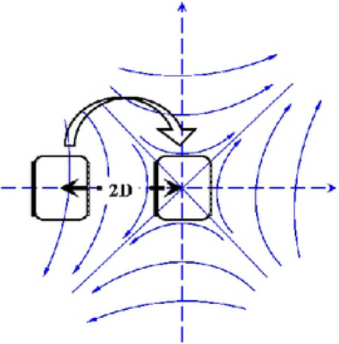
Figure 4: Coil set to measure the gradient and field quality of a quadrupole magnet

0.3.2 The Morgan coil for pulsed magnets

G. H. Morgan [Morgan] proposed a complex coil array that can measure any multipole magnet, or magnet component, in pulsed mode, i.e., with static coil array. Identical coils are located around a cylinder frame with the symmetry to be measured. The number of coils is equal to the multipole order to be measured: three coils for a sextupole, etc.

[b]fig:BNLArray details an array of coils able to measure a large number of harmonics by different connection schemes to put in series the individual coils. Small discrepancies between the individual coils can be eliminated by turning the coil frame at different angular positions. One should not forget that a coil scheme sensitive to a multipole of order $n$ is as well sensitive to order $n\cdot(2m+1)$. Reference [Jain2008] describes the full theory of this technique.

Figure 5: Measuring shaft with 16 individual coils made with printed circuit technology. A large number of harmonics can be measured in pulsed mode by using various connection schemes (courtesy of A. Jain, BNL).

.

0.3.3 A dedicated coil array to measure curved dipoles in pulsed mode: the CNAO fluxmeter

A dedicated array of 11 curved coils has been assembled to measure the CNAO dipole magnets [Rossi2006]. These 1.5 T dipoles have a bending of $22.5^{\degree}$ and operate with a field rise time of 2 seconds. Eddy current effects present in particular in the ends of the magnet yoke have to be taken into account for both the field integral as a function of current and the field quality over the 130 mm useful aperture.

[b]fig:cnaoarray(a) shows the 11 coils fixed on the frame that can be entered from a zero field region into one magnet end to measure the remanent field, or measure in static position during the field ramp [fig:cnaoarray(b)]. A cross-calibration 12th coil can be mounted on top of each individual coil of the fluxmeter. This cross-calibration gave correction factors to equalize the effective width of the 11 coils within $10^{-4}$ relative accuracy.

Note that all correction factors described in sec:realcoil have to be applied to calculate the field errors in terms of multipoles. [b]fig:cnaocurves gives the vertical field component in the horizontal symmetry plane of 10 CNAO dipole magnets measured with this fluxmeter, taking into account these systematic errors.

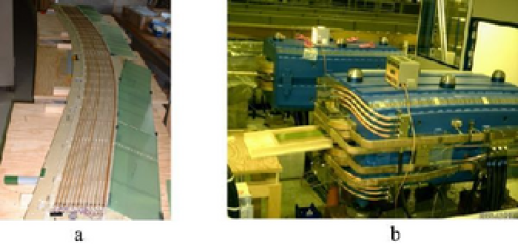
Figure 6: (a) The CNAO fluxmeter with 11 curved coils, (b) inserted in one of the CNAO dipole magnets

0.4 The single stretched wire technique with a dipole magnet

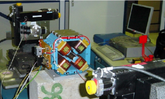
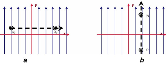
Figure 7: The SSW equipment installed to measure a quadrupole magnet. The wire is displaced in the quadrupole aperture by 2D high-precision stages on both sides.

Figure 8: (a) The single stretched wire displaced horizontally to measure the field integrated over the dipole length. (b) A vertical displacement gives zero signal if displacement and field direction are parallel.

Particle beams are sensitive to field integrated along their trajectory. The SSW (Single Stretched Wire) method consists of a high tensile conducting wire moved inside the magnet aperture by precision displacement tables. CuBe wires 0.1 thick are commonly used. The stages at both sides are assumed to move by precisely the same amount. The return wire is kept fixed, as much as possible in a field-free region. The flux lines crossed during this displacement, $\Psi(x_{1},x_{2})$, and measured by a voltage integrator give the field integrated over the displacement, $d=x_{2}-x_{1}$, and over the SSW length, $L_{\text}{w}$. [b]fig:ssw shows the system developed by FNAL [Dimarco2000] and mounted to measure a quadrupole magnet. When measuring a perfect dipole ($B_{y}=Cst\leavevmode\nobreak\ \leavevmode\nobreak\ ,\leavevmode\nobreak\ \leavevmode\nobreak\ B_{x}=0$) as in fig:sswdipole(a) the integrator gives

$$\Psi(x_{1},x_{2})=\int_{0}^{L}{\int_{x_{1}}^{x_{2}}{B_{y}(x,l)}\cdot dx\cdot dl}=d\cdot\int{B\cdot dl}\leavevmode\nobreak\ .$$ (10)

The measurement accuracy of the dipole strength is linked to the calibration of the integrator gain $(10^{-4}-10^{-5})$ and to the precision of the mechanical displacement. Commercially available stages reach an accuracy better than $10^{-4}=1\Uum\text{/}10\Umm$. This method was cross-checked 30 years ago against NMR mapping and gave agreement within few $10^{-5}$.

Similarly, a vertical displacement in a dipole aligned vertically gives a zero flux variation [see fig:sswdipole(b)]. It is the simplest and most accurate method of finding the field direction of a dipole: accuracies of 0.1 mrad are commonly reached.

This method is simple and efficient to measure the first integral of wigglers and undulators. This first integral value, given by eq:ssw1, corresponds to the angular deflection of the beam and is tuned to be zero in the relevant cross-section of the magnet. It has been complemented by the pulsed wire technique to measure and tune the second field integral value [Ruland1999, Fan2002]. Travelling Hall plate based measurements are nowadays preferred since in addition they give more details on the regularity of the undulator periods.

0.5 Align a quadrupole with the single stretched wire

The single stretched wire technique is relevant to finding the axis, main field direction, and longitudinal position of a quadrupole magnet [Dimarco2000]. These three alignment steps will be treated separately so as to be easily understood. An automated acquisition system is better for iterating changes in the reference position of the wire for both stages according to full measurement cycles until an accurate coincidence between wire and magnet axes is reached.

A pure quadrupolar field is defined by

$$B_{y}=G\cdot x\quad,\quad B_{x}=G\cdot y\leavevmode\nobreak\ .$$ (11)

The magnetic axis is defined by the line where

$$B_{x}=B_{y}=0\leavevmode\nobreak\ .$$ (12)

The main field direction is defined by the symmetry planes:

• $B_{x}=0$ in the horizontal symmetry plane,

• $B_{y}=0$ in the vertical symmetry plane.

Moving a SSW vertically from position $y_{1}$ to position $y_{2}$ [fig:sswquadrupole(a)] gives the measured flux of eq:ssw3, a parabolic dependence. The effective length $L_{\text}{eff}$ hides the integral over the magnet length.

$$\Psi(y_{1},y_{2})=\int_{0}^{L}{\int_{y_{1}}^{y_{2}}{G\cdot y\cdot dy\cdot dl}}=L_{\text}{eff}\cdot\frac{G}{2}\cdot(y_{2}^{2}-y_{1}^{2})\leavevmode\nobreak\ .$$ (13)

A further correction must be applied to take into account the wire sagitta that could reach millimetres for a 10 to 15 m long distance between the stages. The system of fig:ssw incorporates a driver to make the measurement with different wire tensions (fig:tension). The measurement data are extrapolated to infinite tension. This will be detailed in sec:extrapolate since this error source is more detrimental for the measurement of the strength of a quadrupole. To obtain accuracy in the result requires therefore time, even with fully automated equipment and procedures, since loops at different tensions are internal to iteration to align the wire coordinate system to the magnet axis. An accurate measurement of the gradient can only take place after a full alignment procedure.

0.5.1 Align the quadrupole axis and field direction

Figure 9: (a) The single stretched wire displaced vertically in a quadrupole. Two measurements are needed to find the minimum of the parabolic dependency, i.e., the horizontal symmetry plane. (b) The axis and field direction (i.e., tilt of the quadrupole field) are found with eight measurements.

[b]eq:ssw3 tells us that two measurements are needed to find $y_{c}$, minimum of the parabola giving the horizontal plane where the axis is located. The method in use is to measure in an iterative way the fluxes over two equal intervals then displace the central point of the measurement $y_{c}$ until the following condition is reached: