Integrable two-channel $p_{x}+ip_{y}$-wave superfluid model

Abstract

We present a new two-channel integrable model describing a system of spinless fermions interacting through a $p$-wave Feshbach resonance. Unlike the BCS-BEC crossover of the $s$-wave case, the $p$-wave model has a third order quantum phase transition. The critical point coincides with the deconfinement of a single molecule within a BEC of bound dipolar molecules. The exact many-body wavefunction provides a unique perspective of the quantum critical region suggesting that the size of the condensate wavefunction, that diverges logarithmically with the chemical potential, could be used as an experimental indicator of the phase transition.

In recent years $p$-wave paired superfluids have attracted a lot of attention, in part due to their exotic properties Gura1 . Of particular interest is the chiral two-dimensional ($2D$) $p_{x}+ip_{y}$ superfluid of spinless fermions, that supports a topological phase with zero energy Majorana modes Read . The latter are theorized to serve as a basic element for a topological quantum computer Nayak . That exotic superfluid state might be realized in the A1 phase of ³He Volo , in the layered perovskite oxide Sr₂RuO₄ Sarma , and in the Pfaffian quantum Hall state at $\nu=5/2$ filling Moore . Most promising is its realization in a cold gas of fermionic atoms in a single hyperfine state. Indeed, $p$-wave Feshbach resonances have been observed and studied in ⁶Li and ⁴⁰K Fesch with the potential to manipulate the system from the weak (BCS) to the strong (BEC) pairing regime. However, these gases revealed to be unstable due to atom-molecule relaxation processes in which the molecule decays to a deep bound state while the atom escapes with excess energy Levin . Other atomic and molecular gases are now in consideration, as well as different mechanisms to suppress relaxation.

From a theoretical standpoint, despite great efforts to describe these systems, a complete understanding of the BCS-BEC transition and the corresponding phase diagram is still missing. Recently, by means of an exactly solvable $p_{x}+ip_{y}$ pairing model Sierra ; Dunning2010 it was shown that the quantum phase transition (QPT) taking place from weak pairing to strong pairing can be understood as the deconfinement of bound Cooper pairs Romb . In this Letter we introduce an exactly solvable two-channel $p_{x}+ip_{y}$ pairing model with a Feshbach resonance. Our model is exactly solvable in arbitrary dimensions, although we will concentrate on its $2D$ realization. We propose a way to experimentally detect the so-called topological QPT volovik from weak to strong pairing, by measuring a density-density correlation function. This together with the analysis of the size of a Cooper pair in terms of the exact solution allows the characterization of the transition as one of a confinement-deconfinement type without Landau order parameter. Moreover, the transition is shown to be third order in the Ehrenfest classification. Another way to theoretically detect that QPT is by analyzing the behavior of the quantum fidelity $z$ of the ground state wavefunction. Interestingly, the second order derivative of $\ln|z|$ displays a logarithmic singularity at the transition point confirming its third order character.

Consider the $2D$ two-channel $p_{x}+ip_{y}$-wave model

$$H = \sum_{k,k_{x}>0}\frac{|k|^{2}}{2}\left(\hat{n}_{k}+\hat{n}_{-k}\right)+H_{b}$$

$$- g\!\!\!\sum_{k,k_{x}>0}\left[\left(k_{x}+ik_{y}\right)b\,c_{k}^{\dagger}c_{-k}^{\dagger}+\left(k_{x}-ik_{y}\right)b^{\dagger}c_{-k}c_{k}\right],$$

where $c^{\dagger}_{k}$ creates a fermion in mode $k=(k_{x},k_{y})$, $\hat{n}_{k}=c_{k}^{\dagger}c^{\;}_{k}$, $b^{\dagger}$ is a bosonic creation operator, and $H_{b}=\delta\,b^{\dagger}b+g^{2}\,b^{\dagger}b^{\dagger}bb$. Our next goal is to show that this model is a particular realization of a family of exactly-solvable atom-molecule Hamiltonians of physical relevance in the context of cold atom physics.

We start our demonstration by recalling the integrals of motion of the hyperbolic Richardson-Gaudin model Duke1 , which can be generically written as NuclPhysB

$$R_{i} =S_{i}^{z}-$$

$$2\gamma\sum_{j\not=i}\left[\frac{\sqrt{\eta_{i}\eta_{j}}}{\eta_{i}-\eta_{j}}\left(S_{i}^{+}S_{j}^{-}+S_{i}^{-}S_{j}^{+}\right])+\frac{\eta_{i}+\eta_{j}}{\eta_{i}-\eta_{j}}S_{i}^{z}S_{j}^{z}\right],$$

where $S_{i}^{z}$, $S_{i}^{\pm}$, are the three generators of the $SU(2)_{i}$ algebra of mode $i$, $i=0,\cdots,L$, with spin representation $s_{i}$ such that $\langle S_{i}^{2}\rangle=s_{i}(s_{i}+1)$. Therefore, the operators $R_{i}$ contain $L+1$ free parameters $\eta_{i}$ plus the strength of the quadratic term $\gamma$. The integrals of motion (Integrable two-channel $p_{x}+ip_{y}$-wave superfluid model) commute with the $z$ component of the total spin component $S^{z}=\sum_{i=0}^{L}S_{i}^{z}=M-\sum_{i=0}^{L}s_{i}$.

We next single out the copy $i=0$ and consider its large spin $s_{0}$ limit; eventually we are interested in the limit $s_{0}\rightarrow\infty$. The corresponding $SU(2)_{0}$ generators are bosonized by means of the Holstein-Primakoff mapping

$$\!\!\!S_{0}^{z}=b^{\dagger}b-s_{0},\quad S_{0}^{+}=b^{\dagger}\sqrt{2s_{0}-b^{\dagger}b},\quad S_{0}^{-}=(S_{0}^{+})^{\dagger}.$$

In the spin-boson representation the conservation of $S^{z}$ becomes $b^{\dagger}b+\sum_{i=1}^{L}S_{i}^{z}=M-L_{c}/2$, where $L_{c}=2\sum_{i=1}^{L}s_{i}$.

Inserting the boson representation into the integrals of motion and expanding them in terms of $1/s_{0},$ we arrive to the complete set of integrals of motion describing a spin-boson model

$$\mathcal{R}_{0} = H_{b}+\sum_{j}\eta_{j}S_{j}^{z}-g\sum_{j}\sqrt{\eta_{j}}\left(b^{\dagger}S_{j}^{-}+bS_{j}^{+}\right)$$ (3)

$$\mathcal{R}_{i} = \left(\eta_{i}+\frac{\kappa g^{2}}{2}\right)S_{i}^{z}-g^{2}S_{i}^{z}b^{\dagger}b-g\sqrt{\eta_{i}}\left(b^{\dagger}S_{i}^{-}+bS_{i}^{+}\right)$$

$$+ \!\!\!\!\!\!\!\!\!\!g^{2}\sum_{j(\not=i)}\left[\frac{\sqrt{\eta_{i}\eta_{j}}}{\eta_{i}-\eta_{j}}\left(S_{i}^{+}S_{j}^{-}+S_{i}^{-}S_{j}^{+}\right)+\frac{\eta_{i}+\eta_{j}}{\eta_{i}-\eta_{j}}S_{i}^{z}S_{j}^{z}\right],$$

where we took advantage of the freedom to select the values of $\gamma$ and $\eta_{0}$: $\gamma=\frac{1}{2s_{0}}+\frac{\kappa}{4s_{0}^{2}}{\hbox{ and }}\eta_{0}=2g^{2}s_{0}$, so that finite integrals of motion result in the limit $s_{0}\rightarrow\infty$. The detuning parameter $\delta$ in $H_{b}$ is given by $\delta=(L_{c}-2(M-1)-\kappa)g^{2}/2$, with $\kappa$ and $g^{2}$ free parameters.

The corresponding eigenvalues NuclPhysB in this limit are

$$\mathit{r}_{0} = \sum_{\alpha}E_{\alpha}-\sum_{j}\eta_{j}s_{j}$$ (4)

$$\mathit{r}_{i} = s_{i}g^{2}\left(\sum_{j(\not=i)}s_{j}\frac{\eta_{i}+\eta_{j}}{\eta_{i}-\eta_{j}}+\sum_{\alpha}\frac{E_{\alpha}+\eta_{i}}{E_{\alpha}-\eta_{i}}-\frac{\eta_{i}}{g^{2}}-\frac{\kappa}{2}\right).$$

where the set of pair energies (pairons) $E_{\alpha}$ represents a particular solution of the Richardson equations

$$\frac{1}{2g^{2}}+\sum_{i}\frac{s_{i}}{\eta_{i}-E_{\alpha}}-\sum_{\alpha^{\prime}(\not=\alpha)}\frac{1}{E_{\alpha^{\prime}}-E_{\alpha}}=\frac{Q_{o}}{E_{\alpha}},$$ (5)

with $Q_{o}=(M-1)-L_{c}/2+(\delta/2g^{2})$. The exact eigenstates in turn are given by

$$\left|\Psi\right\rangle=\prod\limits_{\alpha=1}^{M}\left(b^{\dagger}+g\sum_{i}\frac{\sqrt{\eta_{i}}}{\eta_{i}-E_{\alpha}}\,S_{i}^{+}\right)\left|0,\nu\right\rangle,$$ (6)

where $\left|0,\nu\right\rangle$ represents the boson vacuum tensor and the state of seniority $\nu$, such that $S^{z}_{i}\left|\nu\right\rangle=-s_{i}\left|\nu\right\rangle$ and $S^{-}_{i}\left|\nu\right\rangle=0$ for all $i$.

This completes the derivation of the integrable spin-boson model defined by the integrals of motion (3), whose eigenvalues and common set of eigenvectors are given by (4) and (6) respectively, expressed in terms of the pair energies $E_{\alpha}$ solutions of the Richardson equations (5).

The connection between the spin-boson model above and the $p_{x}+ip_{y}$ pairing model of Eq. (Integrable two-channel $p_{x}+ip_{y}$-wave superfluid model) is realized by the pair representation of the $SU(2)$ algebra $S_{k}^{z}=\frac{1}{2}\left(\hat{n}_{k}+\hat{n}_{-k}-1\right),~{}S_{k}^{+}=\left(S_{k}^{-}\right)^{\dagger}=(k_{x}+ik_{y})c^{\dagger}_{k}c^{\dagger}_{-k}/\left|k\right|$, where now we consider the mode index to represent momentum $k=(k_{x},k_{y})$. Now $M$ represents the total number of fermionic pairs and bosons and $L_{c}$ is the maximum possible number of fermionic pairs. Inserting this representation in the integral of motion $\mathcal{R}_{0}$ and defining $\eta_{k}=|k|^{2}$ we obtain the Hamiltonian (Integrable two-channel $p_{x}+ip_{y}$-wave superfluid model), $H=\mathcal{R}_{0}$, thus showing that it is exactly solvable. Indeed, any linear combination of the integrals of motion defines an exactly solvable Hamiltonian. In particular, the Hamiltonian studied by Links et al. links2011 , can be obtained from the linear combination $\widetilde{H}=2\sum_{i}\epsilon_{i}\mathcal{R}_{i}$ with $2\epsilon_{i}=1/\eta_{i}$. If $\epsilon_{k}=|k|^{2}/2$, with $0\leqslant k\leqslant k_{\sf cut}$, then the parameters $\eta_{k}$ entering in the Richardson’s equations (5) are defined in the interval $1/|k_{\sf cut}|^{2}=1/(2\omega)\leqslant\eta_{k}\leqslant\infty$. Their exactly solvable model does not display a QPT between the weak and strong pairing phases, because, as stated in Ref. Romb , for the $p_{x}+ip_{y}$ model to display a non-analytic behavior in the continuum limit it is required that one of the parameters $\eta_{k}$ vanishes for a given mode (e.g., $k=0$ mode).

Figure 1: Pairon distribution for $x=-0.1$ (triangles), $x=0.37$ (solid circles) and $x=1.7$ (squares) in a system of $M=10$ pairons, $L_{c}=40$ ($\rho=1/4$), $\lambda=g^{2}L_{c}=1/2$, and $\omega=1$. The open circles represent the five lowest level parameters $\eta_{k}$. The upper inset shows the bosonic, $\rho_{0}$, and fermionic, $\rho-\rho_{0}$, densities for the exact solution (solid line) and the BCS approximation (dashed line). The lower inset displays the exact momentum distribution, $n_{k}$, for the three cases and the BCS approximation in solid lines.

Coming back to the Eqs. (5), in complete analogy with Ref. Romb , we can recognize two special cases. One in which all the pairons $E_{\alpha}$ converge to zero, corresponding to $2Q_{o}+1=M$, and a second case where the first pairon converges to zero, i.e., when $2Q_{o}+1=0$. Defining $x=\delta/(2g^{2}L_{c})$, these two cases correspond to $2x_{\sf MR}=1-(M-1)/L_{c}$ and $2x_{\sf cr}=1-(2M-1)/L_{c}$. The first case defines the so-called Moore-Read line. We will show that the second case signals an interesting third-order QPT.

To get insight into the properties of the different phases we analyze the behavior of the pairons in a finite system. Figure 1 displays the pairon distribution for $x<x_{\sf cr}$ (strong pairing), $x_{\sf cr}<x<x_{\sf MR}$ and $x_{\sf MR}<x$ (weak pairing on both sides of the Moore-Read line) for a system consisting of $M=10$ pairs lying in a disk of radius five units in an otherwise square lattice with $L_{c}=40$ ($\rho\equiv M/L_{c}=1/4$) and $\omega=1$. For $x=1.7$ the system has a fraction of 6 Cooper pairs (complex pairons) and 4 quasi-free pairs states (almost real and positive pairons). Crossing the Moore-Read line, at $x=0.37$, the system is a mixture of 8 Cooper pairs and 2 bound pairs (real an negative pairons). Well inside the strong pairing phase, at $x=-0.1$, all pairs are bound. Therefore, the weak pairing phase is characterized by a mixture of free fermions, Cooper pairs and bound molecules, while the strong pairing phase is a BEC of bound molecules. The upper inset displays the bosonic density, $\rho_{0}=\left\langle b^{\dagger}b\right\rangle/L_{c}$, while the lower inset shows the major rearrangement that takes place in the momentum distribution $n_{k}$ close to $k=0$ between the weak and the strong pairing phases.

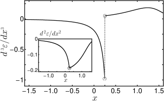
Figure 2: Second (inset) and third-order derivatives of the energy density $\varepsilon$ in the thermodynamic limit ($\rho=1/4,\lambda=1/2$, and $\omega=1$ leading to $x_{\sf cr}=1/4$).

Let us now consider the thermodynamic limit ($L_{c}\rightarrow\infty$ with $\lambda=g^{2}L_{c}$ finite) of this two-channel $p$-wave model. Following the same procedure as in Romb we obtain a pair of couple BCS-like equations for the unknowns $\rho_{0}$ and chemical potential $\mu$

$$x+\rho_{0}-\frac{\mu}{\lambda}=$$ (7)

$$\frac{1}{2\omega}\left[f-|\mu|+\left(\mu-\lambda\rho_{0}\right)\ln\left(\frac{\omega-\mu+\lambda\rho_{0}+f}{\lambda\rho_{0}-\mu+\left|\mu\right|}\right)\right],$$

$$\rho-\rho_{0}=$$ (8)

$$\frac{1}{2}-\frac{1}{2\omega}\left[f-|\mu|-\lambda\rho_{0}\ln\left(\frac{\omega-\mu+\lambda\rho_{0}+f}{\lambda\rho_{0}-\mu+\left|\mu\right|}\right)\right],$$

where $f=\sqrt{2\lambda\omega\rho_{0}+\left(\omega-\mu\right)^{2}}~{}$.

The ground state energy density $\varepsilon=E/L_{c}$ is

$$\varepsilon=\rho(\omega+\mu)+\lambda\rho_{0}x-\left(x-\frac{1}{2}+\rho\right)\frac{\omega\lambda\rho_{0}}{\mu}-\frac{\mu+\left|\mu\right|}{2}.$$

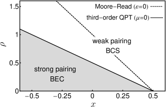
Figure 3: Quantum phase diagram in terms of $\rho$ and $x$, for a fixed value of $\lambda$. Phase boundaries are insensitive to $\lambda$.

If we identify $\lambda\rho_{0}=\Delta^{2}_{\sf BCS}$ and $x=1/2g_{\sf BCS}$, the energy density $\varepsilon$ coincides with the energy density for the one-channel $p_{x}+ip_{y}$ model Romb . Analogously, the right hand sides of Eqs. (7-8) coincide with the corresponding ones in Romb . However, their left hand sides are different due to the existence of two independent parameters $x$ and $\lambda$, or equivalently $\delta$ and $g$. Potential non-analyticities at $\mu=0$ can be attributed to the presence of absolute value of $\mu$ terms. Indeed, from Fig. 2 that shows the second- and third-order derivatives of the energy density with respect to the control parameter $x$, we conclude that the $p$-wave atom-molecule model displays a third-order QPT at the critical value $x_{\sf cr}=\frac{1}{2}-\rho$, coinciding with the limit in which all pairons are real and negative except one that converges to zero, and $\mu=0$. The Moore-Read line corresponds to $x_{\sf MR}=(1-\rho)/2$ and $\mu=\lambda\rho_{0}/2$, leading to $\varepsilon=0$, coinciding with the limit in which all pairons converge to zero. The resulting quantum phase diagram depicted in Fig. 3, depends on the density $\rho$, and on the control parameters $\lambda$ and $x$. However, the phase boundaries are independent of $\lambda$. Thus, our two-channel $p$-wave model extends the one-channel model to: a) $x<0$ due to the possibility of having negative detunings $\delta$, b) $\rho>1$ due to the mixture with a bosonic system, and c) include an extra control parameter $\lambda$.

Since there is no Landau order parameter characterizing this third-order transition, one would like to devise a way to experimentally detect it. In Ref. Romb the root mean square of the condensate wave function was proposed as a possible indicator of that QPT

$$r_{\sf rms}^{2}=\frac{\int|\nabla\phi(k)|^{2}d^{2}k}{\int|\phi(k)|^{2}d^{2}k},$$ (9)

with $\phi(k)\propto\frac{k_{x}+ik_{y}}{\sqrt{(|k|^{2}-a)(|k|^{2}-b)}}$, where $a$ and $b$ are the roots of the polynomial $\xi_{k}^{2}=(\epsilon_{k}-\mu)^{2}+2\lambda\rho_{0}\epsilon_{k}\equiv(\epsilon_{k}-a/2)(\epsilon_{k}-b/2)$. The integral (9) can be obtained analytically. As can be seen in the right inset of Fig. 4, $r_{\sf rms}$ diverges logarithmically at the QPT point as $r_{\sf rms}^{2}\rightarrow-\frac{\ln|\mu/\sqrt{2\omega\lambda\rho_{0}}|}{2\lambda\rho_{0}\ln\left(1+\omega/2\lambda\rho_{0}\right)}$. Making contact with the exact wave function (6) we can immediately associate this divergence to the confinement of the last Cooper pair or, coming from strong pairing, to the deconfinement of a single bound pair within the BEC molecular wave function. Away from the QPT point, $r_{\sf rms}$ diverges again in the extreme weak coupling limit, $x\rightarrow\infty$, in which all pairs are deconfined. The condensate wave function can be related to the density-density correlation function which in coordinate space can be expressed as

$$|\phi(r-r^{\prime})|^{2}=\langle(\hat{n}_{r}-\langle\hat{n}_{r}\rangle)(\hat{n}_{r^{\prime}}-\langle\hat{n}_{r^{\prime}}\rangle)\rangle+|F(r-r^{\prime})|^{2},$$

where $\phi(r-r^{\prime})$ is the condensate wave function in coordinate space, $\hat{n}_{r}=c^{\dagger}_{r}c_{r}$, $\langle\hat{n}_{r}\hat{n}_{r^{\prime}}\rangle$ is the density-density correlation function, and $F(r-r^{\prime})$ is the Fourier transform of the momentum density $\langle\hat{n}_{k}\rangle$. In trapped cold atomic gases, the condensate wave function can be obtained from measurements of the density-density correlations using quantum noise interferometry and the momentum distribution from time-of-flight measurements after opening the trap. Therefore, the root mean square size of the condensate wave function constitutes a unique indicator of the QPT which can be experimentally accessed.

Figure 4: $\chi_{f}/L_{c}$ (see text) as a function of $x$, $\rho=1/4$, $\lambda=1/2$, $\omega=1$ for $\Delta x=10^{-3}$ (dot-dashed) , $5\times 10^{-4}$ (solid), and $10^{-5}$ (dashed). At $x_{\sf cr}=1/4$, as $\Delta x\rightarrow 0$, it diverges logarithmically. At $x=x_{\sf cr}\pm\Delta x$, and finite $\Delta x=5\times 10^{-4}$, the second-order derivative of $\chi$ develops another logarithmic divergence in terms of $\mu$. The root mean square of the Cooper pair size, $r_{\sf rms}$ is shown in the right inset.

The quantum fidelity $z[x,\Delta x]=\langle\Psi(x-\Delta x)|\Psi(x+\Delta x)\rangle$ can also be used as an indicator of QPTs ours1 . The quantity $\chi_{f}=-2\ln|z[x,\Delta x]|/\Delta x^{2}$, which in the limit $\Delta x\rightarrow 0$ is the so-called fidelity susceptibilty, has an essentially different behavior depending on the ground-state overlaps considered. If the overlap is taken between two states belonging to the same phase ($|x-x_{\sf cr}|>\Delta x$), $\chi_{f}/L_{c}$ tends to a value which remains finite in the limit $\Delta x\rightarrow 0$, whereas if the overlap is between two states in different phases ($|x-x_{\sf cr}|\leq\Delta x$) a $\ln\Delta x$ dependence appears. More precisely, $\left.(\chi_{f}/L_{c}\right)|_{x_{\sf cr}}\approx\left.-(d\mu/dx)^{2}\ln(\Delta x)/(\omega\lambda\rho_{0})\right|_{x_{\sf cr}}$. Clearly, when $\Delta x\rightarrow 0$ the fidelity susceptibility develops a logarithmic divergence as a function of $(x-x_{\sf cr})$ similar to that obtained in the one-channel $p_{x}+ip_{y}$ model Dunning2010 .

However, even for $\Delta x$ finite, $\chi_{f}/L_{c}$ shows a non-analytic behavior. When one of the ground-states in $z[x,\Delta x]$ is taken close to the transition point ($x\approx x_{\sf cr}\pm\Delta x$), $\chi_{f}/L_{c}$ can be written as $\left.(\chi_{f}/L_{c})\right|_{x\approx x_{\sf cr}\pm\Delta x}=-\mu_{\mp}^{2}\ln|\mu_{\mp}|/(2\omega\lambda\rho_{0}\Delta x^{2})+\mathcal{O}(\mu_{\mp}^{0})$, with $\mu_{\pm}=\mu(x\pm\Delta x)$. At $x=x_{\sf cr}\pm\Delta x$, where $\mu_{\mp}=\mu(x_{\sf cr})=0$, the previous expression is continuous, but its second-order derivative diverges logarithmically, as shown in Fig. 4. These results should be contrasted with the results obtained for an Ising chain of length $L$ damski , where $\left.(\chi_{I}/L)\right|_{x_{\sf cr}}\approx 1/|\Delta x|$, i.e. power law, and a logarithmic divergence at $x=x_{\sf cr}\pm\Delta x$ appears in the first-order derivative of $\chi_{I}/L$.

In conclusion, we presented a new exactly solvable spin-boson model which has as particular realization the two-channel $p_{x}+ip_{y}$-wave superfluid. We showed that the model has a third order QPT that can be accessed experimentally by measuring the density-density correlation function. The analysis in terms of fidelity provides further evidence of the non-Landau character of the QPT, and its logarithmic singularity indicates that it is of a confinement-deconfinement type, as suggested by the exact wave function.

We acknowledge support from a Marie Curie Action of the European Community Project No. 220335, the Spanish Ministry for Science and Innovation Project No. FIS2009-07277, and the Mexican Secretariat of Public Education Project PROMEP 103.5/09/4482.

References

• (1) V. Gurarie, and L. Radzihovsky, Ann. Phys. 322, 2 (2007).
• (2) N. Read and D. Green, Phys. Rev. B 61, 10267 (2000).
• (3) C. Nayak, et al., Rev. Mod. Phys. 80, 1083 (2008).
• (4) G. E. Volovik, Exotic Properties of Superfluid ${}^{3}He$ (World Scientific, Singapore, 1992).
• (5) S. D. Sarma, C. Nayak, and S. Tewari, Phys. Rev. B 73, 220502(R) (2006).
• (6) G. Moore and N. Read, Nucl. Phys. B 360, 362 (1991).
• (7) C. H. Schunck et al., Phys. Rev. A 71, 045601 (2005); J. P. Gaebler, J. T. Stewart, J. L. Bohn, and D. S. Jin, Phys. Rev. Lett. 98, 200403 (2007).
• (8) J. Levinsen, N. R. Cooper, and V. Gurarie, Phys. Rev. A 78, 063616 (2008).
• (9) M. IbaΓ±ez, J. Links, G. Sierra, and S.-Y. Zhao, Phys. Rev. B 79, 180501 (2009).
• (10) C. Dunning, M. IbaΓ±ez, J. Links, G. Sierra, and S.-Y. Zhao, J. Stat. Mech.: Theory Exp. (2010) P08025.
• (11) S. M. A. Rombouts, J. Dukelsky, and G. Ortiz, Phys. Rev. B 82, 224510 (2010).
• (12) G.Β E. Volovik, Sov. Phys. JETP 67, 1804 (1985).
• (13) J. Dukelsky, C. Esebbag, and P. Schuck, Phys. Rev. Lett. 87, 066403 (2001).
• (14) G. Ortiz, R. Somma, J. Dukelsky, and S. Rombouts, Nucl. Phys. B 707, 421 (2005).
• (15) C. Dunning, P.S. Isaac, J. Links, and S.-Y. Zhao, arXiv:1102.2485.
• (16) For a review see, G. Ortiz in Understanding quantum phase transitions, ed. L. Carr, (CRC Press, Boca Raton, 2010), p. 139, and references therein.
• (17) M. M. Rams and B. Damski, Phys. Rev. Lett. 106, 055701 (2011).