HU-EP-11/19

¹Humboldt-Universität zu Berlin, Institut für Physik,
Newtonstraße 15, D-12489 Berlin, Germany,
²Niels Bohr Institute, Blegdamsvej 17, DK-2100 Copenhagen, Denmark

¹ckalousi@physik.hu-berlin.de, ²dyoung@nbi.dk

Dressed Wilson Loops on $S^{2}$

Chrysostomos Kalousios¹, Donovan Young²

1 Introduction

The Maldacena-Wilson loop [1, 2] has proven to be of pervasive usefulness as an observable in the AdS/CFT correspondence in particular [3], and in the gauge-gravity duality in general. Examples of areas of application include AdS/QCD [4], scattering amplitudes [5], and Dp-brane theories [6, 7, 8]. In Euclidean ${\cal N}=4$ supersymmetric Yang-Mills theory in four dimensions, this non-local, gauge-invariant operator couples both to the gauge field $A_{\mu}(x)$ and to the six real scalar fields $\Phi_{I}(x)$, through the trace of a path-ordered exponential

$$W_{R}(C)=\frac{1}{\dim R(G)}\mathrm{Tr}_{R(G)}{\cal P}\exp\oint d\tau\Bigl{(}i\dot{x}^{\mu}(\tau)A_{\mu}+|\dot{x}(\tau)|\Theta^{I}(\tau)\Phi_{I}\Bigr{)},$$ (1)

where the gauge group is denoted by $G$, $R$ denotes a representation of $G$, and the path $C$ is defined by a closed contour $\{x^{\mu}(\tau),\Theta^{I}(\tau)\}$, where $\Theta^{I}(\tau)\Theta^{I}(\tau)=1$, and so $\Theta^{I}(\tau)$ defines a closed contour on $S^{5}$. The Wilson loop defined in this manner enjoys local supersymmetry, and for contours free of cusps, the scalar coupling removes would-be UV divergences at coincident points along $C$. For particular choices of $\{x^{\mu}(\tau),\Theta^{I}(\tau)\}$, the supersymmetry can be enlarged to a global symmetry of the operator, which leads to great simplifications in the calculation of correlation functions, and in many cases, to results valid for all values of the coupling constant $g_{\text{YM}}$ and the gauge group rank (e.g. $N$ for $G=SU(N)$, which will be the gauge group of interest in what follows).

The AdS/CFT dictionary entry for this object is elegant and simple: the contour $x^{\mu}(\tau)$ resides on the boundary of $AdS_{5}$ and provides a boundary condition for open strings , $\Theta^{I}(\tau)$ provides a similar boundary condition on $S^{5}$. At large $N$ and $\lambda=g^{2}_{\text{YM}}N$, and for $R$ of rank ${\cal O}(1)$, the string worldsheet is classical and describes a minimal surface in $AdS_{5}\times S^{5}$ [17]. The area of this minimal surface is related to the logarithm of the expectation value of the Wilson loop $\langle W_{R}(C)\rangle$. In this way we have replaced the problem of the strong coupling behaviour of $W_{R}(C)$ by one of the most famous problems of the calculus of variations, the Plateau problem, albeit in a curved product space. Moving away from the classical limit, $1/\sqrt{\lambda}$ corrections to $\langle W_{R}(C)\rangle$ may be calculated via semi-classical fluctuation determinants [19, 20, 21, 22, 23, 24, 25, 26, 27, 28].

The simplest Wilson loops (1) have

$$\Theta^{I}(\tau)=M^{I}_{\mu}\,\frac{\dot{x}^{\mu}(\tau)}{|\dot{x}(\tau)|},\qquad M^{I}_{\mu}M^{I}_{\nu}=\delta_{\mu\nu},$$ (2)

and were discovered by Zarembo in [29]. If the curve $x^{\mu}(\tau)$ lies in $\mathbb{R}^{n}$, these Wilson loops are $(1/2)^{n}$-BPS. They have trivial expectation value $\langle W\rangle=1$, to all orders of perturbation theory [30, 31, 32]. The next-to-simplest Wilson loop (1) is the 1/2-BPS circle with contour $\{(\cos\tau,\sin\tau,0,0),\Theta^{I}=\text{const.}\}$ whose dynamics are captured by a Hermitian matrix model [33, 34, 35], exact for all values of $N$ and $\lambda$. Recently, these two examples of Wilson loops were shown to arise from a larger class of generically 1/16-BPS Wilson loops with $x^{\mu}(\tau)\subset S^{3}$, and with scalar coupling given by [36, 37, 38, 39]

$$\Theta^{I}(\tau)=\frac{1}{|\dot{x}|}\sigma^{i}_{\mu\nu}x^{\mu}\dot{x}^{\nu}M_{i}^{I},\qquad M_{i}^{I}M_{j}^{I}=\delta_{ij},$$ (3)

where the tensor $\sigma^{i}_{\mu\nu}$ is defined via the projection of the Lorentz generators in the anti-chiral spinor representation ($\gamma_{\mu\nu}$) onto the Pauli matrices $\tau^{i}$

$$\frac{1}{2}(1-\gamma^{5})\gamma_{\mu\nu}=i\sigma^{i}_{\mu\nu}\tau_{i}.$$ (4)

In the special case when $x^{4}(\tau)=0$, the contour $\vec{x}(\tau)$ resides on a great $S^{2}\subset S^{3}$, the Wilson loops are 1/8-BPS, and $|\dot{\vec{x}}|\Theta^{I}=(\vec{x}\times\dot{\vec{x}},0,0,0)$. Incredibly, these 1/8-BPS loops on $S^{2}$ appear to be captured exactly by the zero-instanton sector of pure Yang-Mills in two-dimensions [40, 41, 42, 43, 44, 45, 46], and therefore by a matrix model. The result for single Wilson loop VEV’s is

$$\langle W\rangle=\frac{1}{N}L_{N-1}^{1}\left(-g_{\text{YM}}^{2}\frac{A_{1}A_{2}}{A^{2}}\right)\exp\left(\frac{g_{\text{YM}}^{2}}{2}\frac{A_{1}A_{2}}{A^{2}}\right),$$ (5)

where $A_{1}$ is the area on $S^{2}$ enclosed by $\vec{x}(\tau)$ and $A_{2}=A-A_{1}$, where $A$ is the total sphere area. When $\vec{x}(\tau)=(\cos\tau,\sin\tau,0)$ one recovers the 1/2-BPS circle and the associated result from the Hermitian matrix model. The limit of a latitude shrinking to zero size at the north pole gives a Zarembo circle, and $\langle W\rangle=1$.

At strong coupling and large-$N$, the 1/8-BPS Wilson loops on $S^{2}$ enjoy a description which is a generalization of the calibrated surfaces technique originally applied to the Zarembo loops at strong coupling in [47]. In particular, the problem of finding classical string solutions of minimal area which end on the 1/8-BPS contours can be reduced to a sigma-model on $S^{3}$ [46]. The procedure is non-trivial however, and not every solution of the sigma-model provides a Wilson loop. Indeed, there were originally only two solutions known, and these were obtained without recourse to the sigma-model: the latitude and the loop formed by two longitudes (i.e. an “orange-wedge”) [39]. The sigma-model allowed a coincident latitude-latitude solution, and an approximate perturbed latitude solution to be found [46]. In the present paper, we will use the dressing method on the longitude solution to find new solutions, whose boundary curves are non-trivial shapes on $S^{2}$. In so-doing we can verify that the regularized area of the worldsheet is in accordance with (5).

This paper is organized as follows. We begin with a review of the pseudo-holomorphicity equations in section 2. In section 3 we review the dressing method and show how the longitude solution is obtained by dressing. We continue in section 4 with a presentation of new solutions obtained by dressing the longitude solution. We conclude in section 5 with a discussion.

2 Pseudo-holomorphicity equations and sigma-model on $S^{3}$

The 1/8-BPS Wilson loops on $S^{2}$ couple to three of the six scalar fields of ${\cal N}=4$ SYM $\vec{\Phi}$

$$W=\frac{1}{N}\mathrm{Tr}\,{\cal P}\exp\oint d\tau\left(i\dot{x}^{\mu}A_{\mu}+(\vec{x}\times\dot{\vec{x}})\cdot\vec{\Phi}\right),$$ (6)

where

$$x^{\mu}=(\vec{x},0),\qquad\vec{x}^{2}=1.$$ (7)

The string duals of these Wilson loops are contained in an $AdS_{4}\times S^{2}$ subspace of $AdS_{5}\times S^{5}$. We write the metric of this subspace as

$$ds^{2}=\frac{1}{z^{2}}dx^{i}dx^{i}+z^{2}dy^{i}dy^{i},\qquad z^{2}=\frac{1}{y^{i}y^{i}},$$ (8)

where $i=1,\ldots,3$, so that $\vec{\theta}\equiv z\vec{y}$ are embedding coordinates for $S^{2}$.

The worldsheets defined by $\{\vec{x}(\sigma,\tau),\,\vec{y}(\sigma,\tau),\,z(\sigma,\tau)\}$ obey first order differential equations (“pseudo-holomorphicity equations”) arising from supersymmetry and some further non-differential constraints [46]. These are as follows

$$\begin{split}\vec{x}^{2}+z^{2}=1,\qquad\vec{x}\cdot\vec{y}=C=\text{const.},\qquad z^{2}\partial_{\alpha}(\vec{x}\times\vec{y})=\epsilon_{\alpha\beta}\partial_{\beta}\vec{x}.\end{split}$$ (9)

It is these relations which allow the problem of finding solutions to be reduced to an auxiliary sigma model on $S^{3}$, supplemented with non-trivial added constraints. One defines the following 4-vector

$$\xi^{A}=(\vec{\xi},\xi^{4}),\qquad\vec{\xi}=z\vec{y}\times\vec{x},\qquad\xi^{4}=\sqrt{1+C^{2}}z.$$ (10)

Using the first two relations of (9), one may show that $\xi^{A}\xi^{A}=1$, and $\xi^{A}$ is therefore contained in an $S^{3}$. Further, by operating $\partial^{2}$ upon $\xi^{A}\xi^{A}$, one obtains

$$\partial^{2}\xi^{A}+\xi^{A}\partial_{\alpha}\xi^{B}\partial_{\alpha}\xi^{B}=0,$$ (11)

which are the equations of motion of the sigma model

$$S=\frac{1}{2}\int d^{2}\sigma\left(\partial_{\alpha}\xi^{A}\partial_{\alpha}\xi^{A}+\Lambda(\xi^{A}\xi^{A}-1)\right).$$ (12)

The last relation in (9) allows one to integrate a solution to the sigma-model in order to obtain $\vec{x}$

$$\partial_{\alpha}\vec{x}=\frac{1}{\sqrt{1+C^{2}}}\epsilon_{\alpha\beta}\left(\xi^{4}\partial_{\beta}\vec{\xi}-\vec{\xi}\partial_{\beta}\xi^{4}\right).$$ (13)

The non-differential constraints can be used to show that

$$\vec{y}=\frac{1}{1-z^{2}}\left(\frac{\vec{x}\times\vec{\xi}}{z}+C\vec{x}\right),$$ (14)

which gives $\vec{y}$ once $\vec{x}$ is known, but only if one ensures that

$$\vec{\xi}\cdot\vec{x}=0,\qquad\vec{x}^{2}+\frac{1}{\vec{y}^{2}}=1,$$ (15)

which are necessary in order to be consistent with (10). These additional constraints greatly constrain the number of solutions to the sigma-model which actually correspond to Wilson loop surfaces. The boundary of the string needs to end on the boundary of $AdS_{5}$ along the Wilson loop contour. This is ensured by the following boundary conditions on $\xi^{A}$

$$\xi^{4}|_{\partial}=0,\qquad\vec{\xi}|_{\partial}=\left.\frac{\dot{\vec{x}}}{|\dot{\vec{x}}|}\right|_{\partial},$$ (16)

where the dot denotes the derivative along the boundary curve.

The regularized area of the worldsheet has a simplified form owing to the pseudo-holomorphicity equations [46]

$$S_{\text{reg.}}=\frac{\sqrt{\lambda}}{4\pi}\int d^{2}\sigma\left(\partial_{a}\vec{\theta}\cdot\partial^{a}\vec{\theta}+\frac{1}{z}\nabla^{2}z\right),$$ (17)

and was shown to be invariant under area-preserving diffeomorphisms, from which one can use known solutions to fix the answer to the result expected from (5), i.e.

$$S_{\text{reg.}}=-\frac{\sqrt{\lambda}}{2\pi}\sqrt{A_{1}A_{2}},$$ (18)

where we remind the reader that $A_{1}$ is the area on $S^{2}$ enclosed by the Wilson loop, and $A_{2}$ is the conjugate area. A corollary of that same analysis showed that

$$C=\pm\frac{A_{2}-A_{1}}{2\sqrt{A_{1}A_{2}}}.$$ (19)

where the $\pm$ refer to the stable/unstable conjugate wrappings of the $S^{2}\subset S^{5}$, see [46] for a discussion. In the body of the paper we will always give the stable solution.

There are two canonical solutions known from the literature. They are the previously mentioned latitude and longitude solutions. The latitude solution is given by

$$\begin{split}&\vec{x}=\sin\theta_{0}\left(\frac{\cos\tau}{\cosh\sigma},\frac{\sin\tau}{\cosh\sigma},\cot\theta_{0}\right),\quad z=\sin\theta_{0}\tanh\sigma,\quad C=\pm\cot\theta_{0},\\ &\xi^{A}=\left(-\frac{\sin\tau}{\cosh\sigma},\frac{\cos\tau}{\cosh\sigma},0,\tanh\sigma\right),\quad\sigma\in[0,\infty],\quad\tau\in[0,2\pi],\end{split}$$ (20)

and $\vec{y}$ is given by (14). This solution is shown in figure 1. The boundary curve $\vec{x}|_{z=0}$ is a latitude at polar angle $\theta_{0}$.

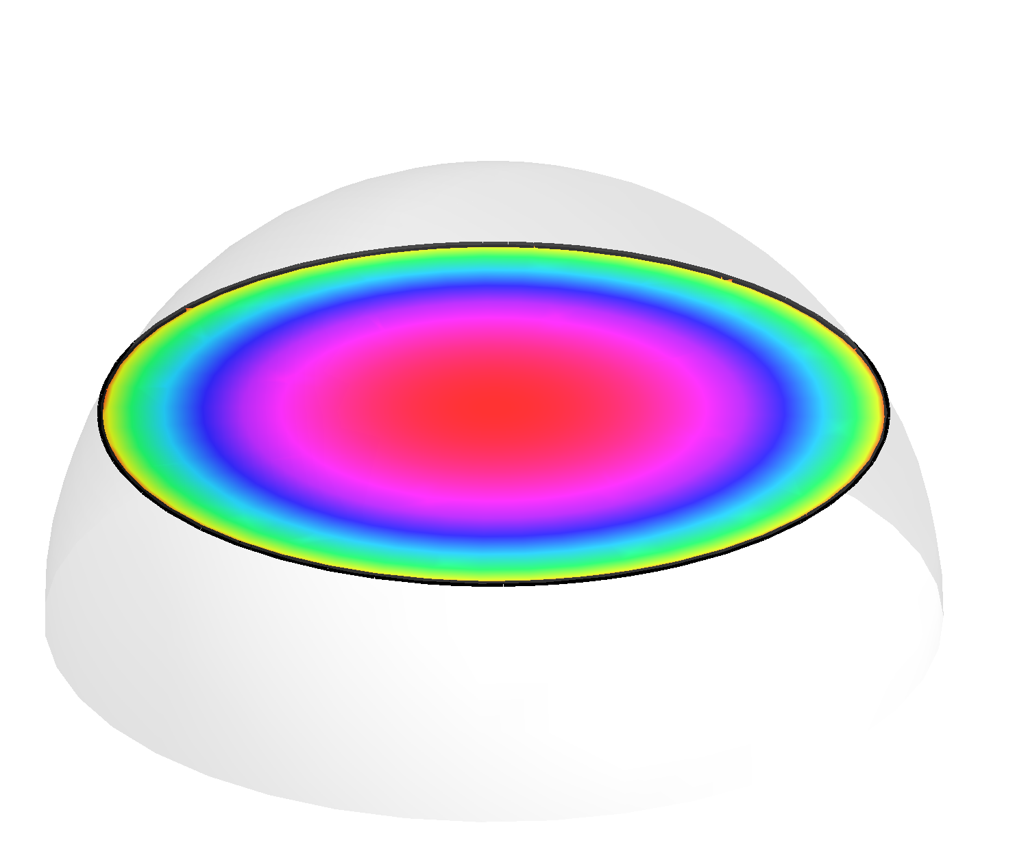
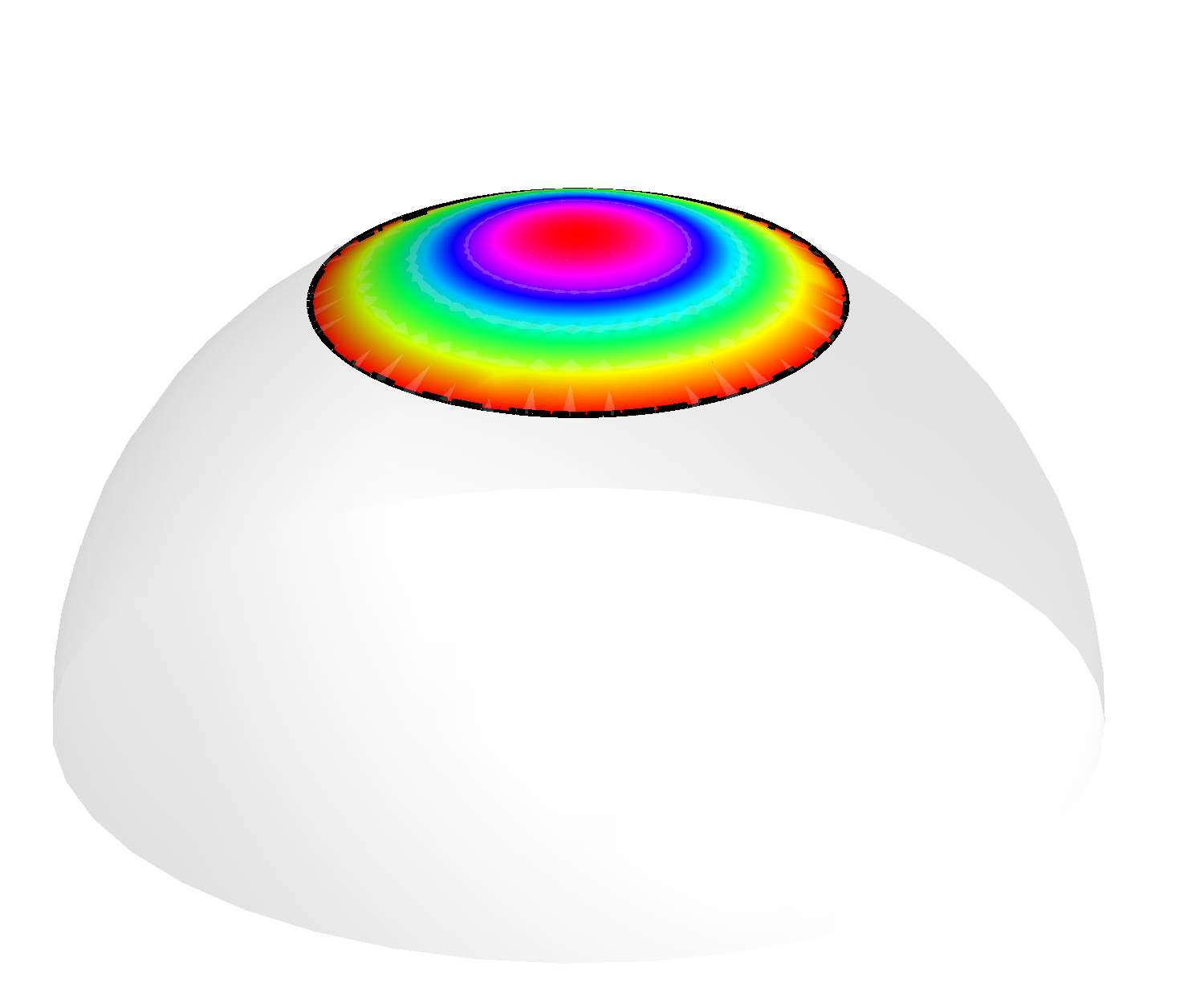
Figure 1: The latitude solution, from left to right: the surface $\vec{x}(\sigma,\tau)$ - its boundary (black curve) lies on the unit $S^{2}$ (shown in gray) $\subset\partial AdS_{5}$; the surface $\vec{\theta}(\sigma,\tau)$ - lying entirely on the unit $S^{2}\subset S^{5}$. The two surfaces are coloured according to the value of the $AdS_{5}$ $z$-coordinate, i.e. by $z(\sigma,\tau)$, whose scale is given in the last plot.

The longitude solution is given by

$$\begin{split}&\vec{x}=\left(\frac{a\sin a\sigma\sin\sigma+\cos a\sigma\cos\sigma}{\cosh\sqrt{1-a^{2}}\tau},\frac{a\cos a\sigma\sin\sigma-\sin a\sigma\cos\sigma}{\cosh\sqrt{1-a^{2}}\tau},-\tanh\sqrt{1-a^{2}}\tau\right),\\ &z=\frac{\sqrt{1-a^{2}}\sin\sigma}{\cosh\sqrt{1-a^{2}}\tau},\quad C=\frac{a}{\sqrt{1-a^{2}}},\quad\sigma\in[0,\pi],\quad\tau\in[-\infty,\infty],\\ &\xi^{A}=\tanh\sqrt{1-a^{2}}\tau\left(-\cos a\sigma,\sin a\sigma,-\frac{\cos\sigma}{\sinh\sqrt{1-a^{2}}\tau},\frac{\sin\sigma}{\sinh\sqrt{1-a^{2}}\tau}\right),\end{split}$$ (21)

which is shown in figure 2. The boundary curve $\vec{x}|_{z=0}$ is given by two longitudes with opening angle $(1-a)\pi$. We will see that the new solutions of section 4 degenerate to this solution in a particular limit. The longitude solution may be obtained by dressing the “vacuum” solution $\xi^{A}=(\sin\tau,\cos\tau,0,0)$ once, as we will show in the next section. The new solutions presented in section 4 are obtained by dressing the vacuum twice, i.e. by dressing the longitude solution.

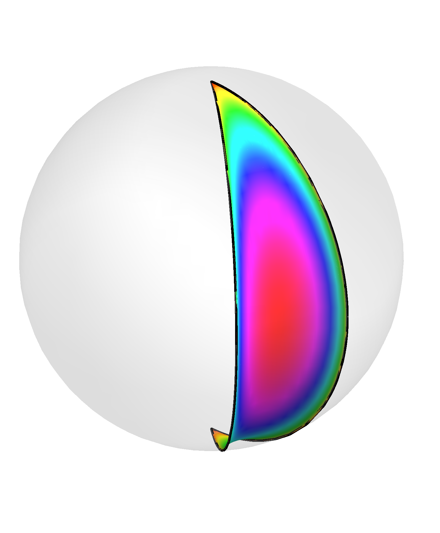
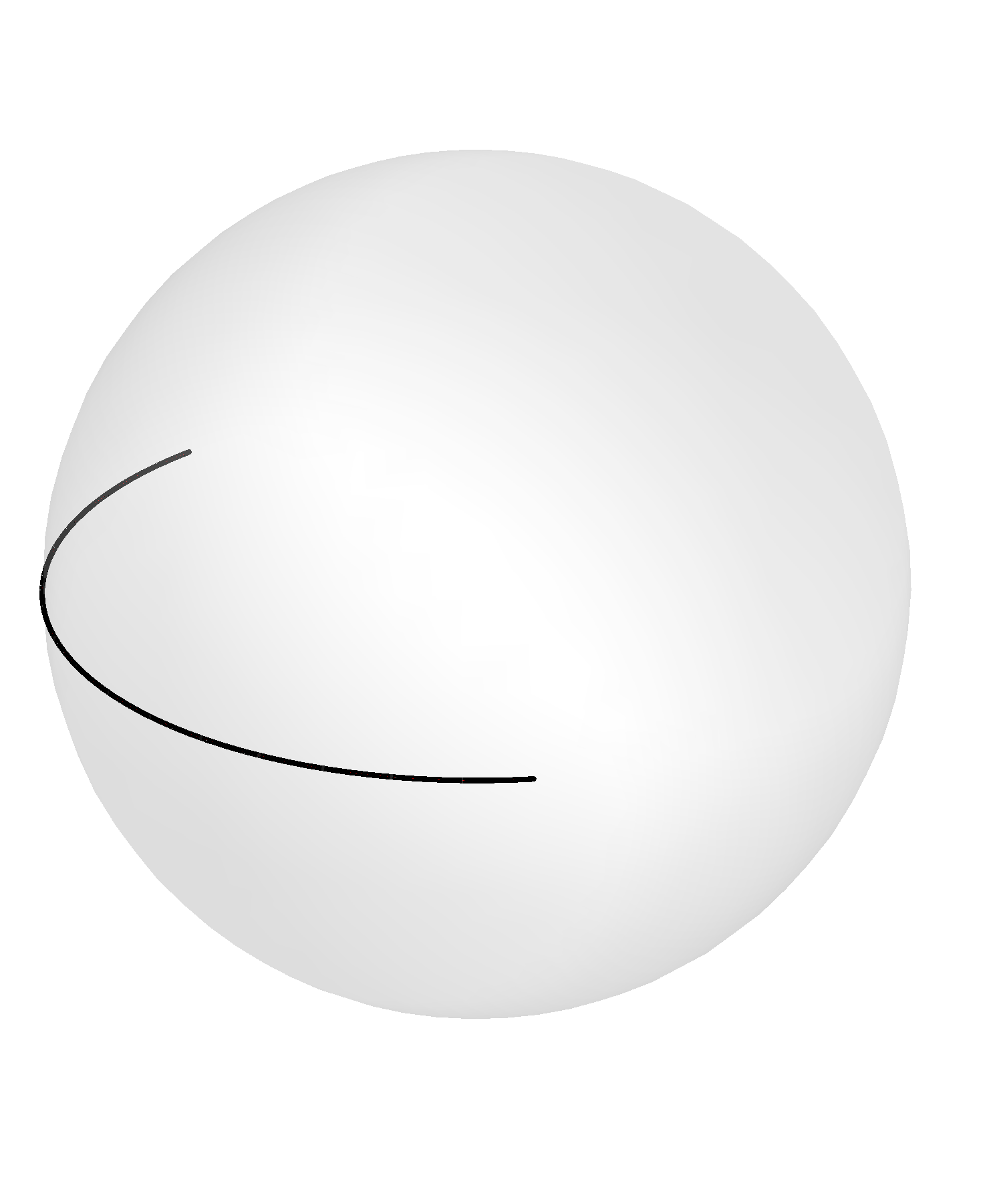
Figure 2: The longitudes solution, from left to right: the surface $\vec{x}(\sigma,\tau)$ - its boundary (black curve) lies on the unit $S^{2}$ (shown in gray) $\subset\partial AdS_{5}$; the surface $\vec{\theta}(\sigma,\tau)$ - lying entirely on the unit $S^{2}\subset S^{5}$. The two surfaces are coloured according to the value of the $AdS_{5}$ $z$-coordinate, i.e. by $z(\sigma,\tau)$, whose scale is given in the last plot.

3 Dressing method

We use the dressing method [48] for the $SU(2)$ sigma model to construct strings that live in $S^{3}$ and have Euclidean worldsheet. Let $\xi^{A}$ be the spacetime components of the string. We consider the element

$$g=\begin{pmatrix}\xi^{1}+i\xi^{2}&-i(\xi^{3}+i\xi^{4})\\ -i(\xi^{3}-i\xi^{4})&\xi^{1}-i\xi^{2}\end{pmatrix}\in SU(2)$$ (22)

and as vacuum we take

$$\xi^{A}=(\sin\tau,~{}\cos\tau,~{}0,~{}0)^{\rm T}.$$ (23)

Going to lightcone coordinates $z_{\pm}=(\sigma\pm i\tau)/2$ we seek a solution to the system of equations

$$\partial_{\pm}\Psi(\lambda)=\frac{\partial_{\pm}gg^{-1}}{1\pm i\lambda}\Psi(\lambda)$$ (24)

subject to the initial condition $\Psi(0)=g$ and the coset constraint $\Psi(\bar{\lambda})^{\dagger}\Psi(\lambda)=I$. We find

$$\Psi(\lambda)=\begin{pmatrix}ie^{-if(\lambda)}&0\cr 0&-ie^{if(\lambda)}\end{pmatrix},\quad f(\lambda)=\frac{\lambda\sigma+\tau}{1+\lambda^{2}}.$$ (25)

The general $N$-soliton solution for the $SU(n)$ sigma model has been constructed in [49] (see also [50, 51, 52]). Here we are interested in the special case $n=2$ and we are focusing only on 1- and 2-soliton solutions, which can be expressed respectively as

$$g_{1}=\sqrt{\frac{\lambda_{1}}{\bar{\lambda}_{1}}}\frac{(\alpha_{11}I_{2\times 2}+h_{1}h_{1}^{\dagger})g_{0}}{\alpha_{11}}$$ (26)

and

$$g_{2}=\sqrt{\frac{\lambda_{1}\lambda_{2}}{\bar{\lambda}_{1}\bar{\lambda}_{2}}}\frac{\left((\alpha_{11}\alpha_{22}-\alpha_{12}\alpha_{21})I_{2\times 2}+\alpha_{22}h_{1}h_{1}^{\dagger}+\alpha_{11}h_{2}h_{2}^{\dagger}-\alpha_{12}h_{1}h_{2}^{\dagger}-\alpha_{21}h_{2}h_{1}^{\dagger}\right)g_{0}}{\alpha_{11}\alpha_{22}-\alpha_{12}\alpha_{21}}.$$ (27)

In the above

$$h_{i}=\Psi(\bar{\lambda}_{i})e_{i},\quad\beta_{ij}=h_{i}^{\dagger}h_{j},\quad\alpha_{ij}=-\frac{\lambda_{i}\beta_{ij}}{\lambda_{i}-\bar{\lambda}_{j}}.$$ (28)

The arbitrary complex vectors $e_{i}$ are called polarization vectors and the complex numbers $\lambda_{i}$ are the spectral parameters of the problem. Once a dressed solution is found, one must then integrate (13) and impose the constraints (9) and (15) to find a Wilson loop solution. In general it is not possible to satisfy these constraints. We have found a two-parameter family of solutions which do lead to Wilson loops, and these are presented in section 4.

3.1 Longitude from dressing

We can reproduce the known longitude solution (LABEL:long) from (26). We choose the polarization vector to be $e_{1}=(1+i,\,1+i)^{\rm T}$ and the spectral parameter $\lambda_{1}=\sqrt{\frac{1+a}{1-a}}\,i$, $|a|<1$. Then we can easily see that the sigma model solution agrees with (LABEL:long).

4 Petal solutions

The twice-dressed vacuum (27) leads to a new two-parameter family of string worldsheets dual to 1/8-BPS Wilson loops. We take the spectral parameters to have only imaginary parts, namely we take $\lambda_{1}=b\,i,~{}\lambda_{2}=i/b$. We choose the polarization vectors to be $e_{1}=(i,~{}-i)^{\rm T},~{}e_{2}=(a\,i,~{}i)^{\rm T}$. The conditions (9) and (15) fix $a$ and the solution is as follows

$$\begin{split}&\vec{x}=\left(\frac{N_{1}}{D},\frac{N_{2}}{D},\frac{N_{3}}{D}+1\right),\quad\xi^{A}=(\vec{\xi},\xi^{4})=\frac{b\sqrt{1+C^{2}}}{D}(Z_{1},Z_{2},Z_{3},Z_{4}),\\ &z=\frac{\xi^{4}}{\sqrt{1+C^{2}}},\quad a=-\frac{1+b^{2}-2b\sqrt{1+C^{2}}}{1+b^{2}+2b\sqrt{1+C^{2}}},\quad\sigma\in[\sigma_{0},\infty],\quad\tau\in\left[0,\pi\frac{b^{2}-1}{b^{2}+1}\right],\end{split}$$ (29)

where $\vec{y}$ is given by (14), $\sigma_{0}$ is given by (32), and where

$$\begin{split}&N_{1}=-(1+a)(b^{4}-1)e^{2b\sigma/(b^{2}-1)}\Bigl{(}a+e^{4b\sigma/(b^{2}-1)}\Bigr{)}\Bigl{(}\sin\frac{2b^{2}\tau}{1-b^{2}}+b^{2}\sin\frac{2\tau}{b^{2}-1}\Bigr{)},\\ &N_{2}=(1+a)(b^{4}-1)e^{2b\sigma/(b^{2}-1)}\Bigl{(}a+e^{4b\sigma/(b^{2}-1)}\Bigr{)}\Bigl{(}\cos\frac{2b^{2}\tau}{1-b^{2}}+b^{2}\cos\frac{2\tau}{b^{2}-1}\Bigr{)},\\ &N_{3}=-(1-a^{2})(1-b^{2})^{2}(1+b^{2})e^{4b\sigma/(b^{2}-1)},\\ &D=b\sqrt{1+C^{2}}\Biggl{[}(1+b^{2})^{2}\left(a^{2}+e^{8b\sigma/(b^{2}-1)}\right)\\ &\qquad+e^{4b\sigma/(b^{2}-1)}\left((1+a^{2})(1-b^{2})^{2}+8ab^{2}\cos\,2\frac{b^{2}+1}{b^{2}-1}\tau\right)\Biggr{]},\end{split}$$ (30)

and where

$$\begin{split}&Z_{1}=(1+b^{2})^{2}\left(a^{2}+e^{8b\sigma/(b^{2}-1)}\right)\sin\tau\\ &\qquad-e^{4b\sigma/(b^{2}-1)}\left((1+a^{2})(1-b^{2})^{2}\sin\tau+4a\left(b^{4}\sin\,\frac{b^{2}+3}{b^{2}-1}\tau+\sin\,\frac{3b^{2}+1}{1-b^{2}}\tau\right)\right),\\ &Z_{2}=(1+b^{2})^{2}\left(a^{2}+e^{8b\sigma/(b^{2}-1)}\right)\cos\tau\\ &\qquad-e^{4b\sigma/(b^{2}-1)}\left((1+a^{2})(1-b^{2})^{2}\cos\tau-4a\left(b^{4}\cos\,\frac{b^{2}+3}{b^{2}-1}\tau+\cos\,\frac{3b^{2}+1}{1-b^{2}}\tau\right)\right),\\ &Z_{3}=-2(1-a)(b^{4}-1)e^{2b\sigma/(b^{2}-1)}\left(a+e^{4b\sigma/(b^{2}-1)}\right)\cos\,\frac{b^{2}+1}{b^{2}-1}\tau,\\ &Z_{4}=2(1+a)(b^{4}-1)e^{2b\sigma/(b^{2}-1)}\left(-a+e^{4b\sigma/(b^{2}-1)}\right)\sin\,\frac{b^{2}+1}{b^{2}-1}\tau.\end{split}$$ (31)

The boundary curve $\vec{x}|_{z=0}$ consists of two longitudes emanating from the north pole, given by $\tau=0$, $\pi(b^{2}-1)/(b^{2}+1)$ and $\sigma\in[\sigma_{0},\infty]$, and a curve connecting their endpoints, given by $\sigma=\sigma_{0}$ and $\tau\in[0,\,\pi(b^{2}-1)/(b^{2}+1)]$, where

$$\sigma_{0}=\frac{(b^{2}-1)}{4b}\log a.$$ (32)

We note that $b$ and $C$ must be chosen so that $a>0$, i.e.

$$\sqrt{1+C^{2}}-C<b<\sqrt{1+C^{2}}+C.$$ (33)

At the special values $b=\sqrt{1+C^{2}}\pm C$ the solution degenerates to the longitude solution (LABEL:long).

The corresponding boundary $\vec{\theta}|_{z=0}=z\vec{y}|_{z=0}$ consists of a curve ending at two points (these points are dual to the longitudes of $\vec{x}|_{z=0}$) and then connected by a longitude (a piece of the equator in this case), which is dual to the point of $\vec{x}|_{z=0}$ at the north pole, i.e. at $\sigma=\infty$. The petal solution is shown in figure 3 for $b=2$ and $C=\sqrt{21}/2$. The parameter $C$ controls the extent to which the “petal” described by $\vec{x}|_{z=0}$ descends away from the north pole. Specifically, the longitudes extend from $x_{3}=1$ (i.e. the north pole) down to $x_{3}=1-(b^{2}-1)^{2}/(2b^{2}C^{2})$. The parameter $b$ controls the opening angle of the longitudes, given by $\pi(b^{2}-1)/(b^{2}+1)$. Several examples of boundary curves are given in figure 4.

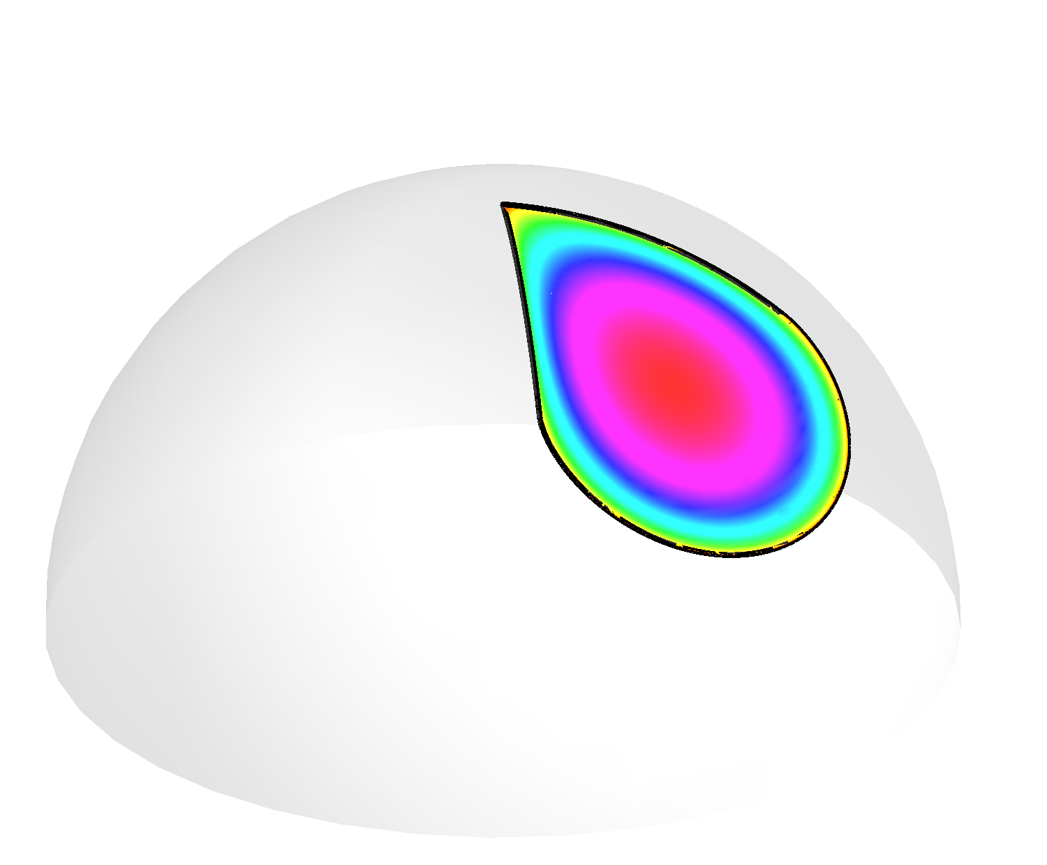
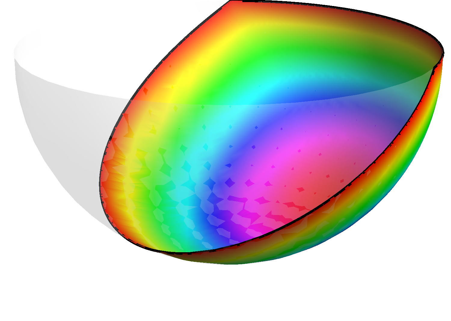
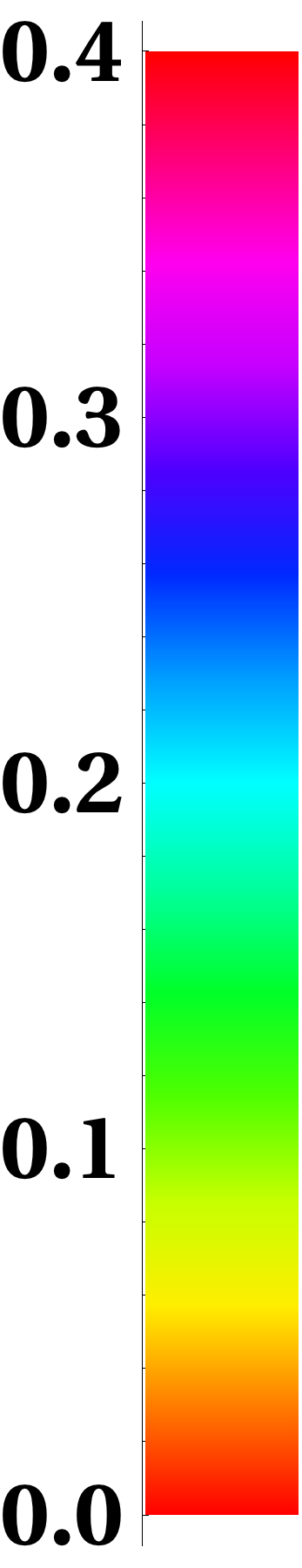
Figure 3: The “petal” solution for $b=2$ and $C=\sqrt{21}/2$, from left to right: the surface $\vec{x}(\sigma,\tau)$ - its boundary (black curve) lies on the unit $S^{2}$ (shown in gray) $\subset\partial AdS_{5}$; the surface $\vec{\theta}(\sigma,\tau)$ - lying entirely on the unit $S^{2}\subset S^{5}$. The two surfaces are coloured according to the value of the $AdS_{5}$ $z$-coordinate, i.e. by $z(\sigma,\tau)$, whose scale is given in the last plot.

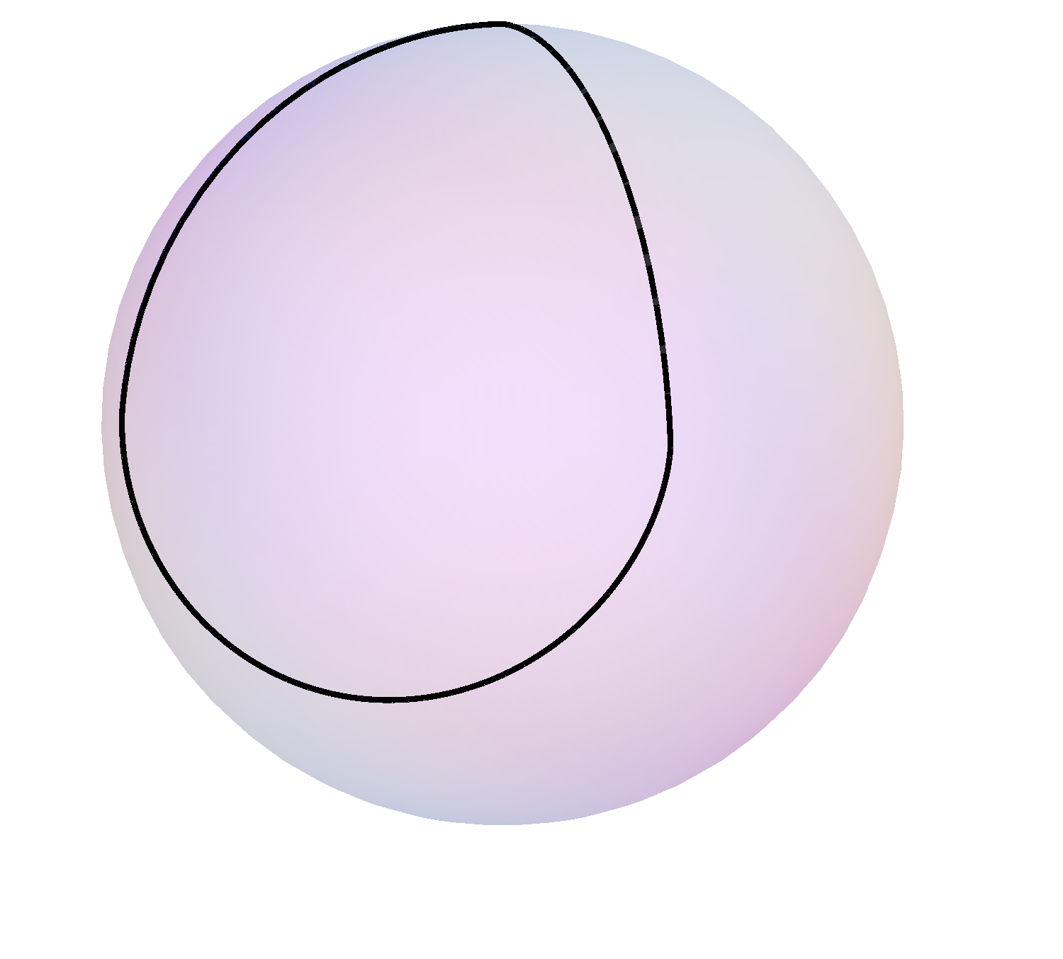
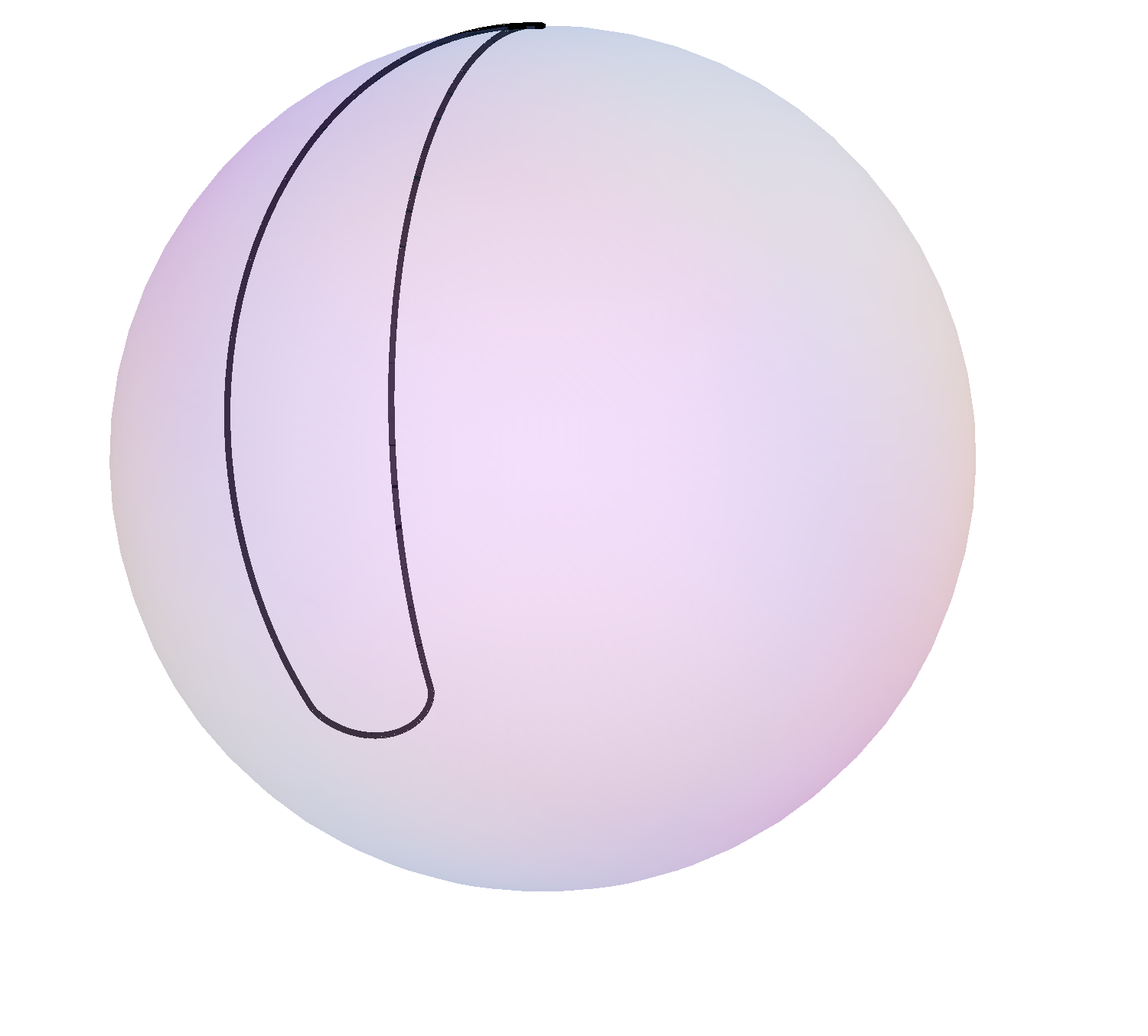
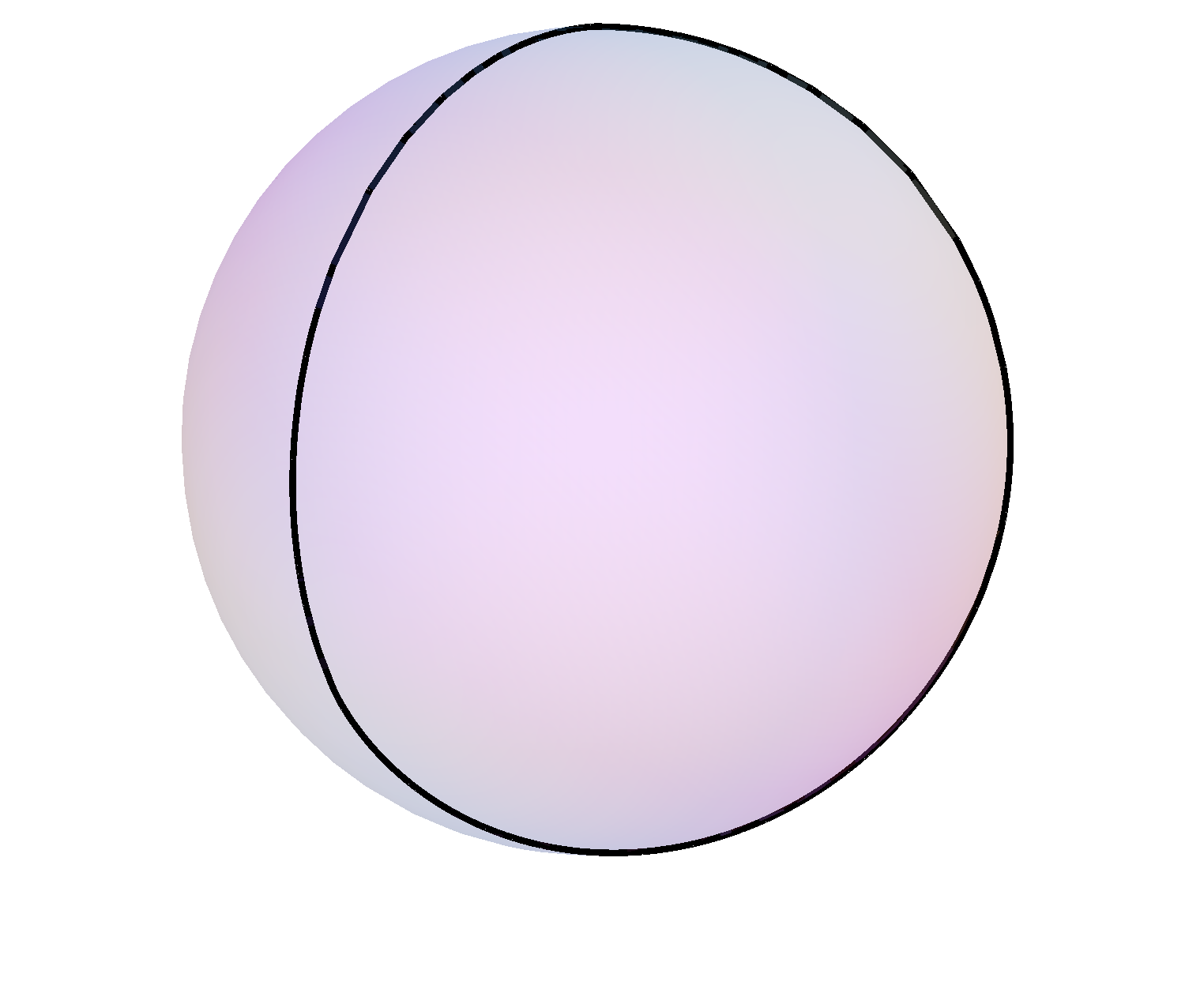
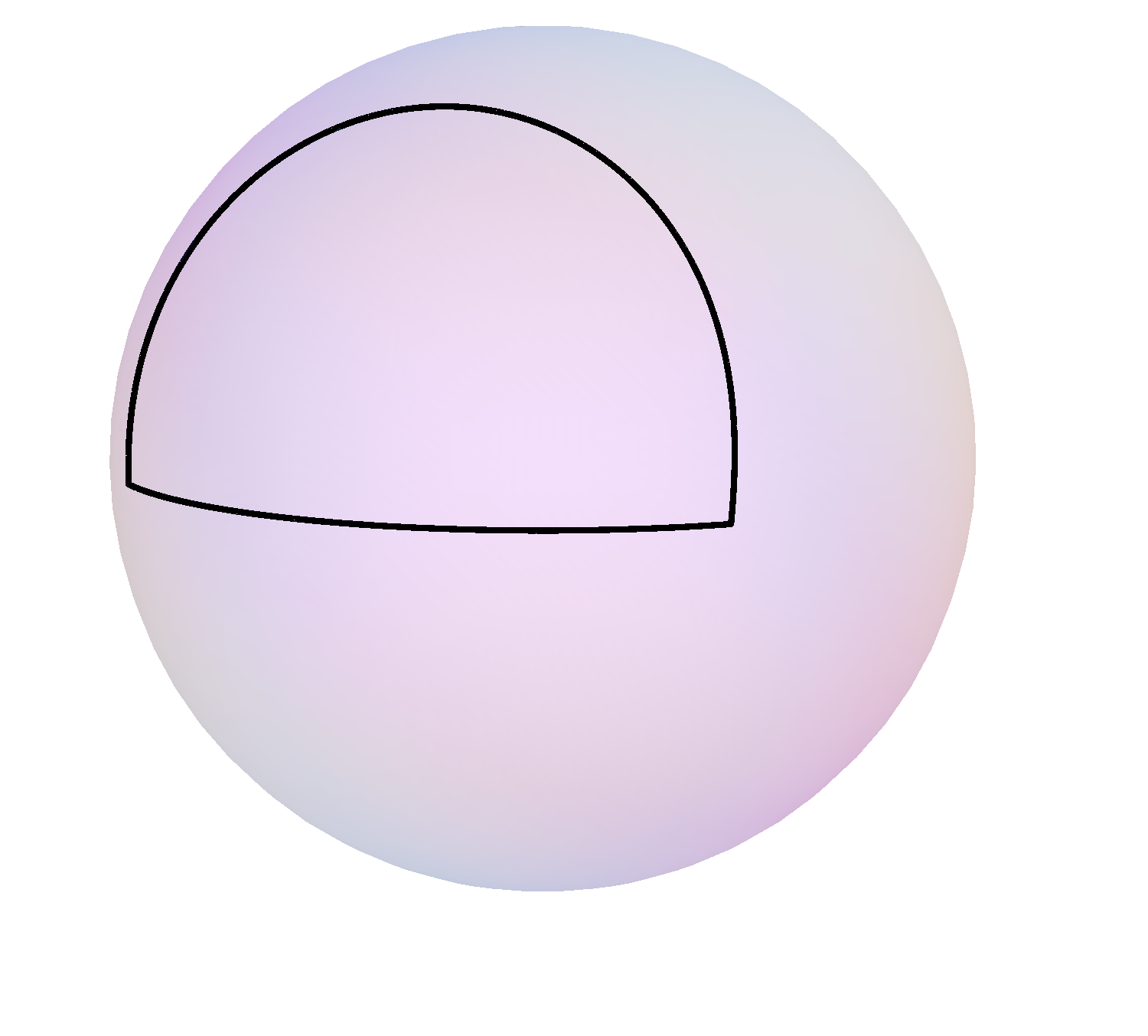
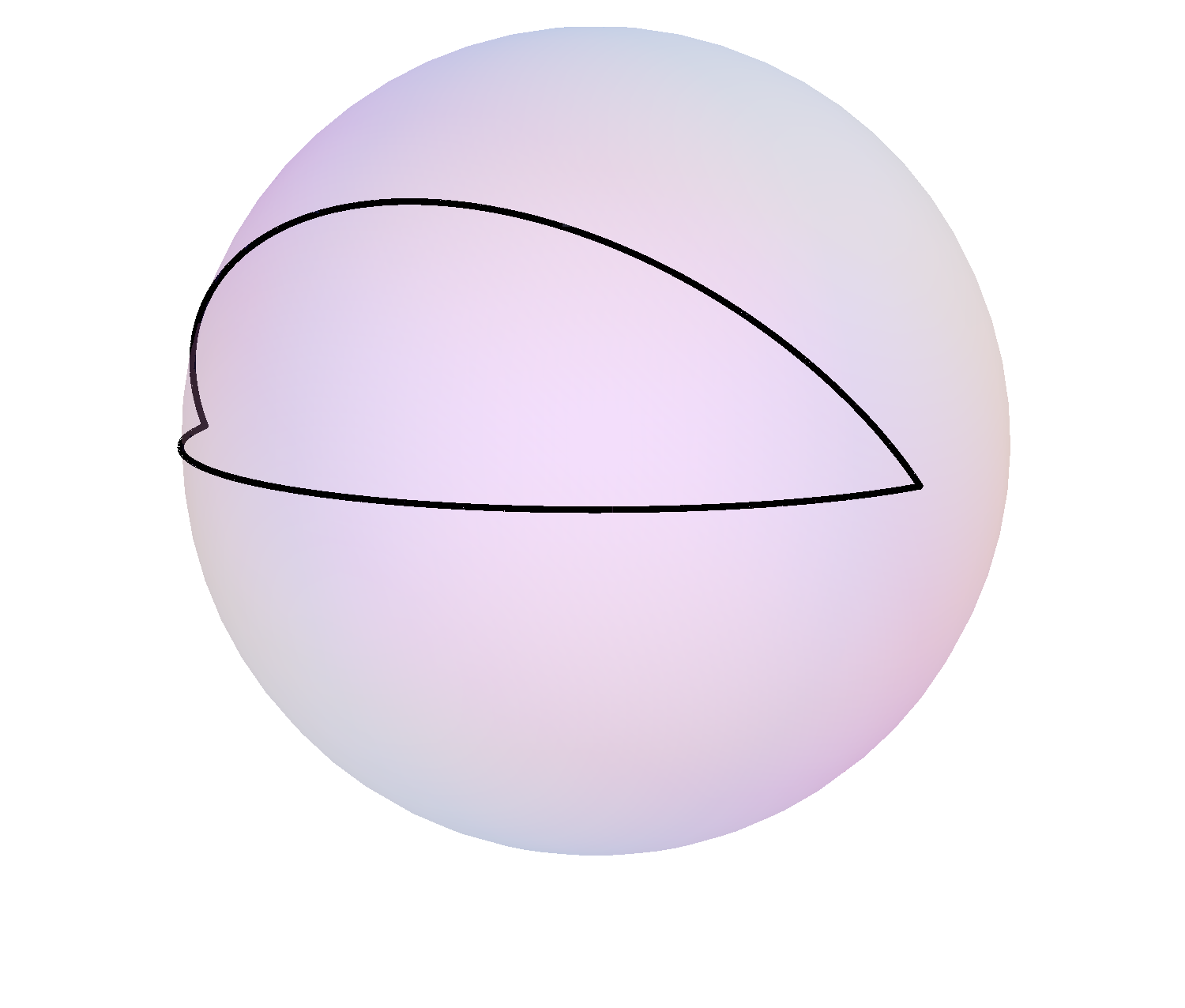
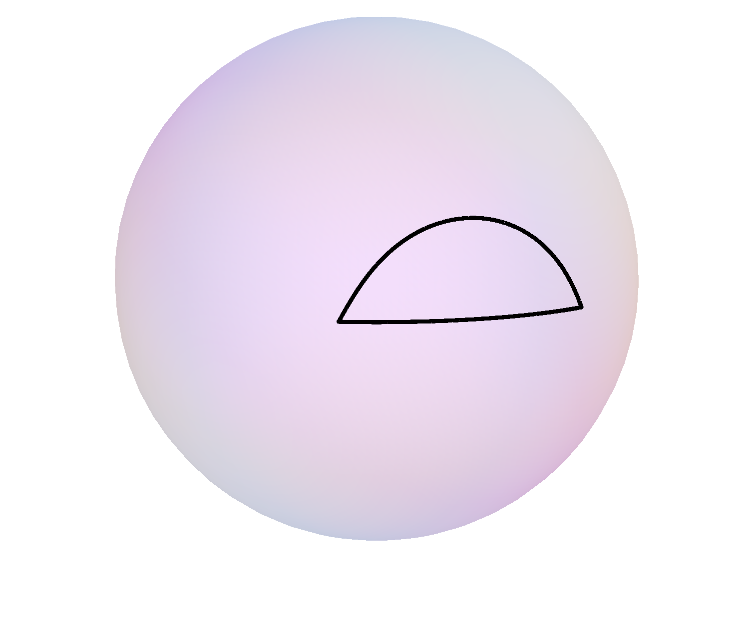
Figure 4: Boundary curves for the petal solution. On the top row $\vec{x}|_{z=0}$ is plotted with $C=0.87$, $1.7$, $0.37$ and $b=0.57$, $3.41$, $1.37$ from left to right respectively. On the bottom row the curves on $S^{5}$, i.e. $\vec{\theta}|_{z=0}$ are given.

4.1 Area enclosed by $\vec{x}|_{z=0}$

It is a simple matter to evaluate the area on $S^{2}$ contained by the boundary curve $\vec{x}|_{z=0}$, since two of the boundaries are longitudes. Using standard spherical polar coordinates

$$\vec{x}|_{z=0}=(\sin\vartheta\cos\varphi,\sin\vartheta\sin\varphi,\cos\vartheta),$$ (34)

the area is given by

$$A_{1}=\int_{0}^{\pi\frac{b^{2}-1}{b^{2}+1}}d\tau\,\dot{\varphi}(\tau)\left(1-\cos\vartheta(\tau)\right),$$ (35)

where $(\vartheta(\tau),\varphi(\tau))$ describes the curve connecting the two longitudes. One finds

$$\begin{split}A_{1}=-&\int_{0}^{\pi\frac{b^{2}-1}{b^{2}+1}}d\tau\,\frac{4(b^{4}-1)^{2}\sin^{2}\,\frac{b^{2}+1}{b^{2}-1}\tau}{\left(1+b^{4}+2b^{2}\cos\,2\frac{b^{2}+1}{b^{2}-1}\tau\right)}\\ &\times\frac{1}{\Bigl{[}(b^{2}-1)^{2}+2(1+b^{4})C^{2}-(1+b^{4}-2b^{2}(1+2C^{2}))\cos\,2\frac{b^{2}+1}{b^{2}-1}\tau\Bigr{]}},\end{split}$$ (36)

which is remarkably free of dependence on $b$, and evaluates to

$$A_{1}=2\pi\left(1-\frac{C}{\sqrt{1+C^{2}}}\right).$$ (37)

We may then verify (19), i.e.

$$\frac{4\pi-2A_{1}}{2\sqrt{(4\pi-A_{1})A_{1}}}=C.$$ (38)

4.2 Regularized area of the worldsheet

According to (18) and (19) we expect that

$$S_{\text{reg.}}=\frac{\sqrt{\lambda}}{4\pi}\int d^{2}\sigma\left(\partial_{a}\vec{\theta}\cdot\partial^{a}\vec{\theta}+\frac{1}{z}\nabla^{2}z\right)=-\frac{\sqrt{\lambda}}{\sqrt{1+C^{2}}}.$$ (39)

Owing to the complexity of $\vec{\theta}(\sigma,\tau)$, the integral is very hard to evaluate in a closed form. However numerical integration works very well if the $b$ parameter is chosen appropriately. We have verified (39) over a wide selection of parameters using numerical integration and have verified it with $10^{-6}$ percent-error accuracy.

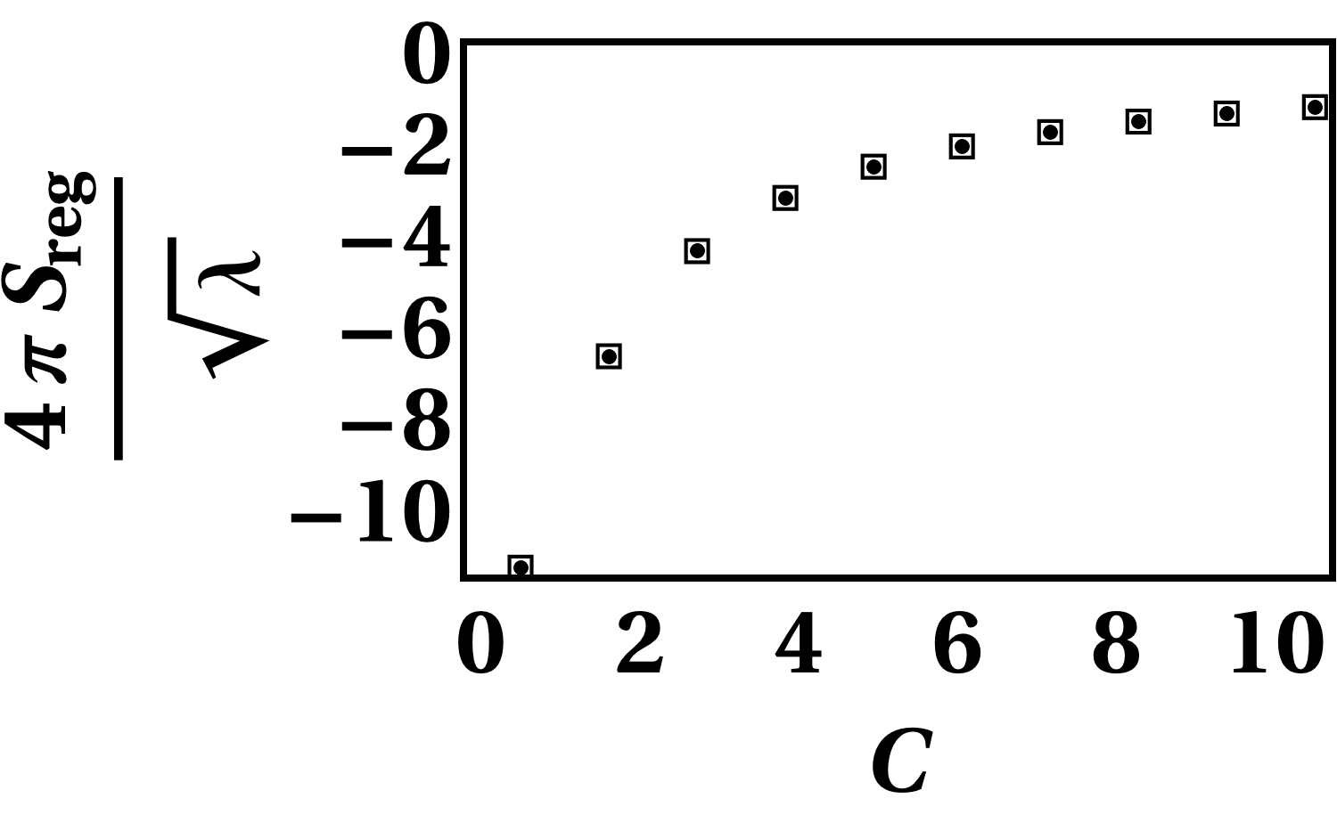
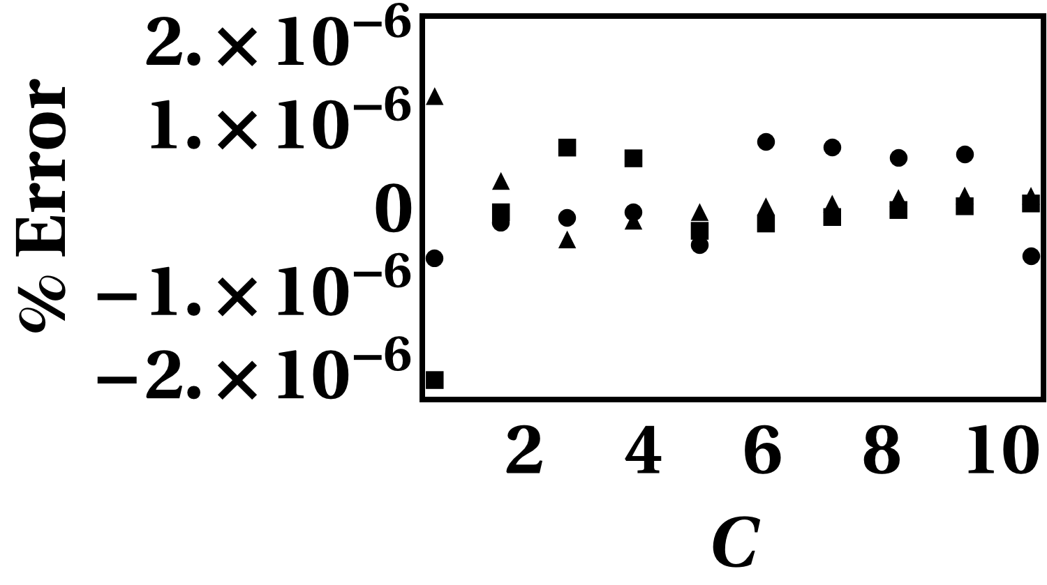
Figure 5: Results from numerical integration of (39). On the left boxes are the prediction given on the RHS of (39) while the dots are the results of numerical integration of the LHS. Each data point represents three numerical integrations where $b$ is set to $\sqrt{1+C^{2}}$ and $\sqrt{1+C^{2}}\pm 3C/5$. The data are not distinguishable by their $b$ values in the plot, i.e. they lie atop one another. The percent error, defined in the text below, is given in the plot on the right: squares indicate $b=\sqrt{1+C^{2}}$, circles $b=\sqrt{1+C^{2}}-3C/5$, and triangles $b=\sqrt{1+C^{2}}+3C/5$.

In figure 5 we show the results of numerical integration performed using the Cuba package [53] for a range of values of $C$, and for each range three representative values of $b$: $\sqrt{1+C^{2}}$ and $\sqrt{1+C^{2}}\pm 3C/5$. In the plot on the left the boxes are the predicted value from the RHS of (39) while the dots are the result of numerical integration of the LHS (the data for each choice of $b$ lie atop one another). The percent error defined as the difference between prediction and numerical integration, divided by prediction, and multiplied by $100$, are also plotted.

5 Discussion

Despite the mapping of the problem of finding string worldsheets corresponding to 1/8-BPS Wilson loops on $S^{2}$ in ${\cal N}=4$ SYM to an auxiliary $\sigma$-model on $S^{3}$, finding explicit solutions is non-trivial. The reason is that the additional constraints (15) greatly constrain the solutions to the $\sigma$-model which correspond to Wilson loops. In this paper we have found a two-parameter family of solutions obtained by using the dressing method on the known longitude solution.

It would be interesting to try the dressing method on different starting solutions, such as the latitude solution, and also to try dressing multiple times. Of course, it would also be very beneficial to attempt to impose the additional constraints in a systematic way, but this seems very difficult.

References

- [1] J. M. Maldacena, “Wilson loops in large N field theories,” Phys.Rev.Lett. 80 (1998) 4859–4862, arXiv:hep-th/9803002 [hep-th].
- [2] S.-J. Rey and J.-T. Yee, “Macroscopic strings as heavy quarks in large N gauge theory and anti-de Sitter supergravity,” Eur.Phys.J. C22 (2001) 379–394, arXiv:hep-th/9803001 [hep-th].
- [3] C. Kristjansen, “Review of AdS/CFT Integrability, Chapter IV.1: Aspects of Non-Planarity,” arXiv:1012.3997 [hep-th].
- [4] J. Casalderrey-Solana, H. Liu, D. Mateos, K. Rajagopal, and U. A. Wiedemann, “Gauge/String Duality, Hot QCD and Heavy Ion Collisions,” arXiv:1101.0618 [hep-th].
- [5] L. F. Alday, “Review of AdS/CFT Integrability, Chapter V.3: Scattering Amplitudes at Strong Coupling,” arXiv:1012.4003 [hep-th].
- [6] A. Brandhuber, N. Itzhaki, J. Sonnenschein, and S. Yankielowicz, “Wilson loops in the large N limit at finite temperature,” Phys.Lett. B434 (1998) 36–40, arXiv:hep-th/9803137 [hep-th].
- [7] A. Agarwal and D. Young, “Supersymmetric Wilson Loops in Diverse Dimensions,” JHEP 0906 (2009) 063, arXiv:0904.0455 [hep-th].
- [8] S. Chakraborty and S. Roy, “Wilson loops in (p+1)-dimensional Yang-Mills theories using gravity/gauge theory correspondence,” arXiv:1103.1248 [hep-th].
- [9] N. Drukker and B. Fiol, “All-genus calculation of Wilson loops using D-branes,” JHEP 0502 (2005) 010, arXiv:hep-th/0501109 [hep-th].
- [10] J. Gomis and F. Passerini, “Holographic Wilson Loops,” JHEP 0608 (2006) 074, arXiv:hep-th/0604007 [hep-th].
- [11] J. Gomis and F. Passerini, “Wilson Loops as D3-Branes,” JHEP 0701 (2007) 097, arXiv:hep-th/0612022 [hep-th].
- [12] S. A. Hartnoll and S. Kumar, “Higher rank Wilson loops from a matrix model,” JHEP 0608 (2006) 026, arXiv:hep-th/0605027 [hep-th].
- [13] S. A. Hartnoll, “Two universal results for Wilson loops at strong coupling,” Phys.Rev. D74 (2006) 066006, arXiv:hep-th/0606178 [hep-th].
- [14] S. Yamaguchi, “Wilson loops of anti-symmetric representation and D5-branes,” JHEP 0605 (2006) 037, arXiv:hep-th/0603208 [hep-th].
- [15] S. Yamaguchi, “Bubbling geometries for half BPS Wilson lines,” Int.J.Mod.Phys. A22 (2007) 1353–1374, arXiv:hep-th/0601089 [hep-th].
- [16] O. Lunin, “On gravitational description of Wilson lines,” JHEP 0606 (2006) 026, arXiv:hep-th/0604133 [hep-th].
- [17] N. Drukker, D. J. Gross, and H. Ooguri, “Wilson loops and minimal surfaces,” Phys.Rev. D60 (1999) 125006, arXiv:hep-th/9904191 [hep-th].
- [18] R. Ishizeki, M. Kruczenski, and S. Ziama, “Notes on Euclidean Wilson loops and Riemann Theta functions,” arXiv:1104.3567 [hep-th].
- [19] J. Greensite and P. Olesen, “Remarks on the heavy quark potential in the supergravity approach,” JHEP 9808 (1998) 009, arXiv:hep-th/9806235 [hep-th].
- [20] Y. Kinar, E. Schreiber, J. Sonnenschein, and N. Weiss, “Quantum fluctuations of Wilson loops from string models,” Nucl.Phys. B583 (2000) 76–104, arXiv:hep-th/9911123 [hep-th].
- [21] S. Forste, D. Ghoshal, and S. Theisen, “Stringy corrections to the Wilson loop in N=4 superYang-Mills theory,” JHEP 9908 (1999) 013, arXiv:hep-th/9903042 [hep-th].
- [22] N. Drukker, D. J. Gross, and A. A. Tseytlin, “Green-Schwarz string in AdS(5) x S**5: Semiclassical partition function,” JHEP 0004 (2000) 021, arXiv:hep-th/0001204 [hep-th].
- [23] M. Kruczenski, R. Roiban, A. Tirziu, and A. A. Tseytlin, “Strong-coupling expansion of cusp anomaly and gluon amplitudes from quantum open strings in AdS(5) x S**5,” Nucl.Phys. B791 (2008) 93–124, arXiv:0707.4254 [hep-th].
- [24] R. Roiban and A. A. Tseytlin, “Strong-coupling expansion of cusp anomaly from quantum superstring,” JHEP 0711 (2007) 016, arXiv:0709.0681 [hep-th].
- [25] M. Kruczenski and A. Tirziu, “Matching the circular Wilson loop with dual open string solution at 1-loop in strong coupling,” JHEP 0805 (2008) 064, arXiv:0803.0315 [hep-th].
- [26] S.-x. Chu, D. Hou, and H.-c. Ren, “The Subleading Term of the Strong Coupling Expansion of the Heavy-Quark Potential in a N=4 Super Yang-Mills Vacuum,” JHEP 0908 (2009) 004, arXiv:0905.1874 [hep-ph].
- [27] V. Forini, “Quark-antiquark potential in AdS at one loop,” JHEP 1011 (2010) 079, arXiv:1009.3939 [hep-th].
- [28] A. Faraggi and L. A. Zayas, “The Spectrum of Excitations of Holographic Wilson Loops,” arXiv:1101.5145 [hep-th].
- [29] K. Zarembo, “Supersymmetric Wilson loops,” Nucl.Phys. B643 (2002) 157–171, arXiv:hep-th/0205160 [hep-th].
- [30] Z. Guralnik and B. Kulik, “Properties of chiral Wilson loops,” JHEP 0401 (2004) 065, arXiv:hep-th/0309118 [hep-th].
- [31] Z. Guralnik, S. Kovacs, and B. Kulik, “Less is more: Non-renormalization theorems from lower dimensional superspace,” Int.J.Mod.Phys. A20 (2005) 4546–4553, arXiv:hep-th/0409091 [hep-th].
- [32] A. Kapustin and E. Witten, “Electric-Magnetic Duality And The Geometric Langlands Program,” arXiv:hep-th/0604151 [hep-th].
- [33] J. Erickson, G. Semenoff, and K. Zarembo, “Wilson loops in N=4 supersymmetric Yang-Mills theory,” Nucl.Phys. B582 (2000) 155–175, arXiv:hep-th/0003055 [hep-th].
- [34] N. Drukker and D. J. Gross, “An Exact prediction of N=4 SUSYM theory for string theory,” J.Math.Phys. 42 (2001) 2896–2914, arXiv:hep-th/0010274 [hep-th].
- [35] V. Pestun, “Localization of gauge theory on a four-sphere and supersymmetric Wilson loops,” arXiv:0712.2824 [hep-th].
- [36] N. Drukker, “1/4 BPS circular loops, unstable world-sheet instantons and the matrix model,” JHEP 0609 (2006) 004, arXiv:hep-th/0605151 [hep-th].
- [37] N. Drukker, S. Giombi, R. Ricci, and D. Trancanelli, “More supersymmetric Wilson loops,” Phys.Rev. D76 (2007) 107703, arXiv:0704.2237 [hep-th].
- [38] N. Drukker, S. Giombi, R. Ricci, and D. Trancanelli, “Wilson loops: From four-dimensional SYM to two-dimensional YM,” Phys.Rev. D77 (2008) 047901, arXiv:0707.2699 [hep-th].
- [39] N. Drukker, S. Giombi, R. Ricci, and D. Trancanelli, “Supersymmetric Wilson loops on S**3,” JHEP 0805 (2008) 017, arXiv:0711.3226 [hep-th].
- [40] A. Bassetto, L. Griguolo, F. Pucci, and D. Seminara, “Supersymmetric Wilson loops at two loops,” JHEP 0806 (2008) 083, arXiv:0804.3973 [hep-th].
- [41] D. Young, “BPS Wilson Loops on S**2 at Higher Loops,” JHEP 0805 (2008) 077, arXiv:0804.4098 [hep-th].
- [42] A. Bassetto, L. Griguolo, F. Pucci, D. Seminara, S. Thambyahpillai, et al., “Correlators of supersymmetric Wilson-loops, protected operators and matrix models in N=4 SYM,” JHEP 0908 (2009) 061, arXiv:0905.1943 [hep-th].
- [43] A. Bassetto, L. Griguolo, F. Pucci, D. Seminara, S. Thambyahpillai, et al., “Correlators of supersymmetric Wilson loops at weak and strong coupling,” JHEP 1003 (2010) 038, arXiv:0912.5440 [hep-th].
- [44] S. Giombi and V. Pestun, “Correlators of local operators and 1/8 BPS Wilson loops on S**2 from 2d YM and matrix models,” JHEP 1010 (2010) 033, arXiv:0906.1572 [hep-th].
- [45] V. Pestun, “Localization of the four-dimensional N=4 SYM to a two-sphere and 1/8 BPS Wilson loops,” arXiv:0906.0638 [hep-th].
- [46] S. Giombi, V. Pestun, and R. Ricci, “Notes on supersymmetric Wilson loops on a two-sphere,” JHEP 07 (2010) 088, arXiv:0905.0665 [hep-th].
- [47] A. Dymarsky, S. S. Gubser, Z. Guralnik, and J. M. Maldacena, “Calibrated surfaces and supersymmetric Wilson loops,” JHEP 0609 (2006) 057, arXiv:hep-th/0604058 [hep-th].
- [48] V. E. Zakharov and A. V. Mikhailov, “Relativistically Invariant Two-Dimensional Models in Field Theory Integrable by the Inverse Problem Technique. (In Russian),” Sov. Phys. JETP 47 (1978) 1017–1027.
- [49] C. Kalousios and G. Papathanasiou, “Giant Magnons in Symmetric Spaces: Explicit -soliton solutions for , and ,” JHEP 07 (2010) 068, arXiv:1005.1066 [hep-th].
- [50] J. P. Harnad, Y. Saint Aubin, and S. Shnider, “Superposition of solutions to Bäcklund transformations for the principal sigma model,” J. Math. Phys. 25 (1984) 368.
- [51] M. Spradlin and A. Volovich, “Dressing the Giant Magnon,” JHEP 0610 (2006) 012, arXiv:hep-th/0607009 [hep-th].
- [52] C. Kalousios, G. Papathanasiou, and A. Volovich, “Exact solutions for N-magnon scattering,” JHEP 0808 (2008) 095, arXiv:0806.2466 [hep-th].
- [53] T. Hahn, “CUBA: A library for multidimensional numerical integration,” Comput. Phys. Commun. 168 (2005) 78–95, arXiv:hep-ph/0404043.