Universality in Fluid Domain Coarsening: The case of vapor-liquid transition

Abstract

Domain growth during the kinetics of phase separation is studied following vapor-liquid transition in a single component Lennard-Jones fluid. Results are analyzed after appropriately mapping the continuum snapshots obtained from extensive molecular dynamics simulations to a simple cubic lattice. For near critical quench interconnected domain morphology is observed. A brief period of slow diffusive growth is followed by a linear viscous hydrodynamic growth that lasts for an extended period of time. This result is in contradiction with earlier inclusive reports of late time growth exponent $1/2$ that questions the uniqueness of the non-equilibrium universality for liquid-liquid and vapor-liquid transitions.

I Introduction

Understanding non-equilibrium evolution during the phase separation in a system is of fundamental importance BRAY ; HAASEN ; WADHAWAN ; JONES and of much research interest, both theoretically and experimentally HORBACH ; DAS ; DAS_PURI ; MITCHELL ; BUCIOR ; YELASH ; HORE ; MAJUMDER ; KENDON ; THAKRE ; KABREDE ; DAS2 ; BLONDIAUS ; LIU ; AHMAD ; SICILIA ; KHANNA ; ZANNETTI . Upon quenching from a high temperature homogeneous state to a temperature below the critical point, the system becomes unstable to fluctuations and starts phase separating with the formation and usually nonlinear growth of particle rich and particle depleted domains. Such coarsening is a scaling phenomenon STAUFFER , e.g., the shape functions characterizing the morphology obey the scaling relations BRAY ; HAASEN ; WADHAWAN ; SICILIA ; STAUFFER

$$C(r,t) \equiv \tilde{C}(r/\ell(t)),$$ (1)

$$S(k,t) \equiv \ell(t)^{d}\tilde{S}(k\ell(t)),$$ (2)

$$P(\ell_{d},t) \equiv \ell(t)^{-1}\tilde{P}[\ell_{d}/\ell(t)],$$ (3)

where $C(r,t)$, $S(k,t)$ and $P(\ell_{d},t)$ are respectively the two-point equal-time correlation function, structure factor and domain size distribution function. In Eqs. (1-3) $\tilde{C}(x)$, $\tilde{S}(y)$ and $\tilde{P}(z)$ are the master functions independent of time ($t$)-dependent average domain-size $\ell(t)$ that typically grows in a power law manner

$$\ell(t)\sim t^{\alpha}.$$ (4)

The growth exponent $\alpha$, in Eq. (4), depends upon the transport mechanism driving the phase separation. For diffusive dynamics, associating the domain growth with the chemical potential gradient as

$$\frac{d\ell(t)}{dt}\sim\lvert\overrightarrow{\nabla}\mu\lvert\sim\frac{\gamma}{\ell(t)^{2}},$$ (5)

$\gamma$ being the inter-facial tension, one obtains $\alpha=1/3$. This is referred to as the Lifshitz-Slyozov LIFSHITZ (LS) law. While LS law is the only expected behavior for phase separating solid mixtures, one expects much faster growth, at large length scales, for fluids and polymers, where hydrodynamics is important. Compared to the kinetics in vapor-liquid phase separation, domain coarsening in binary fluids received much more attention HORBACH ; DAS ; DAS_PURI ; HORE ; KENDON ; THAKRE ; AHMAD ; SHINOZAKI ; DUNWEG ; MA ; TOXVAERD where following consensus for the behavior of late stage growth SIGGIA ; FURUKAWA ; FURUKAWA1 ; ONUKI has been reached in $d=3$. Considering a balance between the surface energy density $(\gamma/\ell(t))$ and the viscous stress ($6\pi\eta v_{\ell}/\ell(t)$, $v_{\ell}$ being the interface velocity and $\eta$ the shear viscosity) for an interconnected domain structure, one can write

$$\frac{d\ell(t)}{dt}=v_{\ell}=\frac{\gamma}{\eta}.$$ (6)

Solution of Eq. (6) predicts a linear growth ($\alpha=1$), a picture that holds for low Reynolds number. However, for $\ell(t)\gg\ell_{in}(=\eta^{2}/(\rho\gamma)$, $\rho$ being the density), the inertial length, the surface energy density is balanced by kinetic energy density $\rho v_{\ell}^{2}$, so that

$$\frac{d\ell(t)}{dt}\sim\frac{1}{\ell(t)^{1/2}},$$ (7)

giving $\alpha=2/3$. Note that $\alpha=1$ is referred to as the viscous hydrodynamic growth and $\alpha=2/3$ as inertial hydrodynamic growth. While crossover from diffusive to viscous hydrodynamic regime was observed in molecular dynamics (MD) simulations AHMAD ; TOXVAERD and experiments CHOU ; WONG ; BATES , both viscous and inertial growths were observed in lattice-Boltzmann simulations WADHAWAN .

While non-equilibrium universality for vapor-liquid phase separation is expected to be the same as the liquid-liquid, rare inclusive MD simulations that exist KABREDE ; ABRAHAM ; KOCH ; YAMAMOTO ; NAKANISHI for the vapor-liquid transition report an exponent $\alpha=1/2$ for late time domain coarsening. Thus, even though our recent focus has turned to systems with realistic interactions and physical boundary conditions HORBACH ; DAS ; DAS_PURI ; MITCHELL ; BUCIOR ; YELASH ; HORE , our basic knowledge and understanding of segregation kinetics in bulk fluids still remains a challenge. In this letter, we present results from large scale MD simulations for kinetics of vapor-liquid phase separation in a single-component Lennard-Jones (LJ) fluid. This work reports first observation of viscous hydrodynamic growth via MD simulation, thus computationally confirming that the non-equilibrium universality class of vapor-liquid and liquid-liquid phase separation is indeed the same as in the case of equilibrium critical phenomena for both static and dynamic properties.

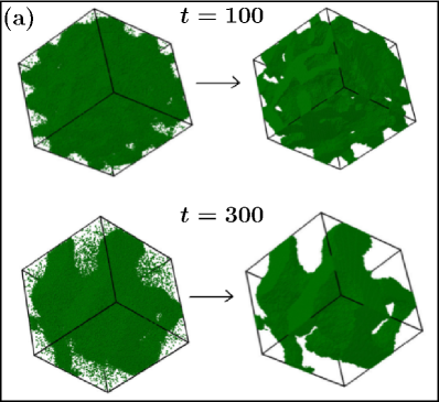
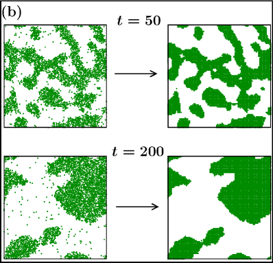
Figure 1: (a) Left frames show the $3-d$ snapshots during evolution of the vapor-liquid phase separation in a simple Lennard-Jones system, at two different times, as indicated. The total density was set to $0.3$ that gives interconnected domain morphology,as seen. The simulation was performed after quenching a homogeneous system prepared at a high temperature to a temperature $T=0.7$. The right panel corresponds to the same snapshots, but after removing the noise (see text for details) to obtain a pure domain morphology. (b) Cross-sectional view of the same system in $xy$ plane at two other times. Here also the left frames show the original snapshots and the right ones show the same after removing noise.

II Model and Method

We consider a model where particles interact via

$$V(r_{ij})=U(r_{ij})-U(r_{c})-(r_{ij}-r_{c})\left(\frac{dU(r_{ij})}{dr_{ij}}\right)_{r_{ij}=r_{c}},$$ (8)

with

$$U(r_{ij})=4\epsilon\left[\left(\frac{\sigma}{r_{ij}}\right)^{12}-\left(\frac{\sigma}{r_{ij}}\right)^{6}\right]$$ (9)

being the standard LJ potential. In Eqs. (8) and (9) $r_{ij}$ is the scalar distance between the $i$th and $j$th particles, $\sigma$ is the particle diameter and $\epsilon$ is the interaction strength. The cut-off and shifting of the potential at $r_{c}$ was used to faclitate faster computation. Further, introduction of the third term Allen on the right hand side ensures that both the effective potential and force are continuous at $r_{c}$ which was set to $2.5\sigma$. All particles were assigned equal mass $m$. For the sake of convenience, below we set $m,~{}\sigma,~{}\epsilon$ and $k_{B}$ to unity.

The phase-diagram of the model without the force-correction term is known Smit , the critical temperature ($T_{c}$) and critical density ($\rho_{c}$) being $1.085\pm 0.005$ and $0.317\pm 0.006$ respectively. It is understood, of course, that the introduction of force-correction will somewhat change the value of $T_{c}$, which, from our experience Das_Horbach ; Das_Fisher ; Sutapa with a similar model that was used to study phase-separation in binary mixture, could be approximately $10\%$ lower. In this work we have chosen the temperature low enough so that even without the complete knowledge of the critical parameters, we are safely below the co-existence curve, as is also clear from the nice phase-separating domain pattern shown in Fig. 1. The interconnected nature of the morphology also ensures that our choice of overall density ($\rho$) is close to the critical value. In a future correspondence, of course, we will undertake the understanding of the phase behavior of this model in conjunction with the presentation of detailed results on the phase-separation kinetics at various temperatures and densities.

A total $265421$ particles were confined in a periodic $3$-dimensional box of linear dimension $L=96$. Thus we worked with a density $\rho=0.3$. The MD runs were performed using the Verlet velocity algorithm FRENKEL ; Allen with an integration time step of $\Delta t=0.005\tau$, $\tau=(m\sigma^{2}/\epsilon)^{1/2}=1$. The temperature $T$ was controlled by using a Nosé-Hoover thermostat (NHT) FRENKEL , which is known to preserve hydrodynamics well. At $t=0$ homogeneous initial configurations, prepared by equilibrating the system at $T=5$, were quenched to $T<T_{c}$. All the results were obtained by averaging over $5$ independent runs at a quench temperature $T=0.7$.

The left frames of Fig. 1(a) are typical $3$-dimensional evolution pictures from two different times where the black dots represent a particle. They demonstrate nice interconnected structure of segregating domains growing with time. The average density of liquid and vapor domains are respectively $0.72$ and $0.02$. A direct method to characterize the structure is to calculate the radial distribution function, $g(r)$, from these continuum configurations. However, we are interested in looking at $C(r,t)$, its Fourier transform $S(k,t)$ and $P(\ell_{d},t)$ which have been more standard tools in the study of phase ordering dynamics. To facilitate the calculation of latter quantities, we map the continuum snapshots to a lattice one in such a way that a pure domain structure is obtained where all lattice sites inside a liquid domain have occupancy one while sites inside the vapor domain have occupancy zero. An appropriate renormalization procedure MAJUMDER ; DAS2 ; AHMAD is applied for this noise removal exercise. We further map this system into spin-$1/2$ Ising system where an occupied lattice site has spin value $S_{i}=1$ and for a vacant site $S_{i}=-1$. The right frames in Fig. 1(a) show such mapped configurations. In Fig. 1(b) we demonstrate similar exercise by showing cross-sectional views at two other times. Which may be difficult to appreciate from the $3-d$ snapshots, these $2-d$ pictures clearly show that no significant structural change has occurred during this transformation that can hamper the analysis. Also during the entire duration of study, we find that the composition of up and down spins remains conserved within a tolerable limit of $5\%$ fluctuations.

From the mapped configurations, the correlation function $C(r)$ is calculated as

$$C(r,t)=\langle S_{i}S_{j}\rangle~{}-~{}\langle S_{i}\rangle^{2},$$ (10)

where the angular brackets stand for statistical averaging. The average domain size $\ell(t)$ from the decay of $C(r,t)$ was estimated as

$$C(r=\ell(t),t)=h,$$ (11)

where $h$ was set to the first zero of $C(r,t)$. Other methods employed for the calculation of $\ell(t)$ are

$$\ell(t)=\frac{1}{\int dk~{}kS(k)}$$ (12)

and

$$\ell(t)=\int d\ell_{d}\ell_{d}P(\ell_{d},t).$$ (13)

In Eqs. (12) and (13), it is assumed that $S(k,t)$ and $P(\ell_{d},t$) are appropriately normalized. In Eq. (13), $\ell_{d}$ is obtained from the separation between two successive domain interfaces in $x-$, $y-$ or $z-$ directions.

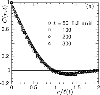
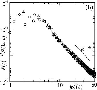
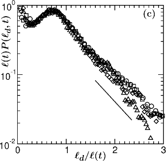
Figure 2: Scaling plot of (a) $C(r,t)$ vs $r/\ell(t)$ (b) $\ell(t)^{-d}S(k,t)$ vs $k\ell(t)$ and (c) $\ell(t)P(\ell_{d},t)$ vs $\ell_{d}/\ell(t)$ where data from four different times, as indicated, have been collapsed. All quantities were calculated from noise-free domain structures. The continuous line in (b) corresponds to the Porod law while the one in (c) represents an exponential decay of the tail.

III Results

In Fig. 2(a), we present the scaling plot of $C(r,t)$ vs. $r/\ell(t)$ for which four different times were chosen, as indicated on the figure. While collapse of data from the earliest time with the other ones is not good, excellent data collapse with three later times is indicative that a scaling regime is reached. In Fig. 2(b) we show the scaling behavior of $S(k,t)$ on a log-log plot. The parallel nature of the tail region to the continuous line confirms consistency with the Porod law POROD ; OONO_PURI . Fig. 2(c) shows the scaling plot of $P(\ell_{d},t)$ on a semi-log plot where the linear behavior of the tail region is consistent with an exponential decay DAS2 ; SICILIA . Note that in all the cases, $\ell(t)$ used was obtained from Eq. (13). The nice data collapse obtained in all the quantities by using $\ell(t)$ from a single measure speaks about the consistency of different methods. Henceforth all the results for $\ell(t)$ will be presented after calculating via Eq. (13).

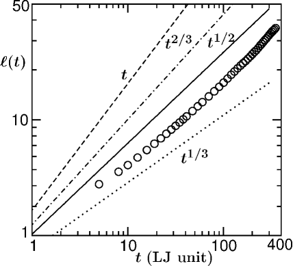
Figure 3: Plot of $\ell(t)$ vs $t$ on a log-scale. All data were obtained after removing the noise as described in the text. Here different lines correspond to growth laws $\ell(t)\sim t^{1/3},~{}t^{1/2},~{}t^{2/3}$ and $t$, as indicated.

Coming to the central objective of the paper, viz., quantifying the dynamics, in Fig. 3 we present plot of $\ell(t)$ vs. $t$ on a log scale. There various lines correspond to various growth laws in domain coarsening problem. While the early time data is more consistent with a diffusive growth ($\alpha=1/3$), there appears a gradual crossover to a faster growth. The intermediate time data, of course, look consistent with $t^{1/2}$ as reported in previous works KABREDE ; ABRAHAM ; KOCH ; YAMAMOTO ; NAKANISHI and at a later time there seems to be a further crossover. However, due to large offset at the crossover region(s), which will be clearer from further analysis and discussions, we warn the reader not to take this conclusion seriously. For similar reasons, an apparently $t^{1/3}$ looking behavior during early time should also not be taken seriously. In fact, due to this and other practical difficulties, it is advisable not to reach a firm conclusion from looking at the behavior on a log-scale (which, of course, is a standard practice followed in the literature), unless one has results over several decades in time and length.

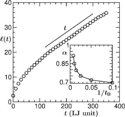
Figure 4: Plot of $\ell(t)$ vs $t$ on a linear scale. All data were obtained after removing the noise as described in the text. The solid line corresponds to the expected linear growth in the viscous hydrodynamic regime. Inset: Plot of the growth exponent $\alpha$, as a function of $1/t_{0}$, obtained by fitting the data in (a) to the form (14) in the range [$t_{0}$,$350$].

Fig. 4 shows a plot of $\ell(t)$ vs $t$ on a linear scale where the data starting from $t\simeq 100$ look quite linear all the way till the end. The deviation from this linear behavior at early time ($t<100$) could be attributed to slower diffusive growth, as discussed above. A fitting to the form,

$$\ell(t)=A+Bt^{\alpha},$$ (14)

however, in the range $t~{}\epsilon~{}[0,100]$ gives $\alpha=0.66$. Since this diffusive regime is short lived and also accompanied by gradual crossover to a faster growth regime, it is in fact not practical to search for growth exponent $\alpha=1/3$ in this region. On the other hand, a similar fitting to the range $t~{}\epsilon~{}[100,350]$ gives $\alpha\simeq 0.9$, quite consistent with the predictions for viscous hydrodynamic growth. Note that for $t>350$ one hits the finite-size effects for the system size used in this work. In the inset of Fig. 4 we present plot of the exponent $\alpha$ as a function of $1/t_{0}$ obtained by fitting the data to the form (14) in the range [$t_{0}$,$350$]. This exercise conclusively says that the exponent at late time certainly is larger than $1/2$ which was reported earlier. Even though in the main frame of Fig. 4 one sees a linear behavior for an extended period of time, for the sake of completeness and to further strengthen our claim we take the following route which, in addition to being a nice exercise, could be useful for other complex situations.

In Fig. 5 we present a plot of instantaneous exponent $\alpha_{i}$ calculated as HUSE

$$\alpha_{i}=\frac{d[\ln\ell(t)]}{d[\ln t]},$$ (15)

vs $1/\ell(t)$. Due to the off-set ($\ell_{0}$) at $t=0$, as discussed in the context of Fig. 3, $\alpha_{i}$ is less than unity for the whole range. However it seems to be approaching unity in a non-linear fashion. The dashed line there with an arrow at the end serves as a guide to the eyes. The lower part in this figure represents the corresponding result obtained from MD simulation by using Andersen thermostat (AT) FRENKEL . Due to the stochastic nature of this thermalization algorithm, it is expected that a diffusive growth will be seen for all time and lengthscales and indeed is seen. There the dashed line has the form MAJUMDER

$$\alpha_{i}=\frac{1}{3}\left[1-\frac{\ell_{0}}{\ell(t)}\right],$$ (16)

which says that the observation of $\alpha<1/3$ for finite domain lengths is a mathematical artifact coming due to non-zero value of $\ell_{0}$ and does not necessarily mean that the actual exponent is not $1/3$ at early time. Coming to the point of hydrodynamic preserving capability of NHT, of course, much better thermostats are available these days. However, from the difference seen for the results coming from NHT and AT, it is clear that NHT is preserving it rather well. Thus the validity of the methodology adopted in this work is justified.

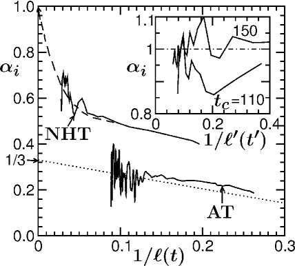
Figure 5: Plot of instantaneous exponent $\alpha_{i}$ vs $1/\ell(t)$. The dashed line is a guide to the eyes, while the dotted line corresponds to Eq. (16). Inset: Plot of $\alpha_{i}$ vs $1/\ell^{\prime}(t^{\prime})$ for two different values of $t_{c}$, as indicated. There the horizontal line represents there the linear hydrodynamic growth.

Note that in Eq. (16) $\ell_{0}$ corresponds to the characteristic length scale at the beginning of a scaling regime and not necessarily the length at $t=0$. In situations where one does not expect multiple scaling regimes (as is the case with AT) $\ell_{0}$ can be nicely estimated from a data-collapse experiment in finite-size scaling analysis MAJUMDER ; MAJUMDER2 . But situation is more complex with NHT due to a crossover to hydrodynamic regime and non-availability of data for different system sizes. However, considering that the crossover, at time $t_{c}$, under discussion is to a linear regime, confirmation about it could be obtained by using the following simpler method. To start with, we assume that the growth obeys a power law behavior as a function of the shifted time $t^{\prime}=t-t_{c}$ as

$$\ell^{\prime}(t^{\prime})=\ell(t)-\ell(t_{c})=At^{\prime\alpha}$$ (17)

and calculate the instantaneous exponent

$$\alpha_{i}=\frac{d[\ln\ell^{\prime}(t^{\prime})]}{d[\ln t^{\prime}]}.$$ (18)

Eq. (17) is invariant under an arbitrary choice of $t_{c}$ if we are in a linear growth regime and one should obtain a constant value $\alpha_{i}=1$ for all choices of $t_{c}$ in the post crossover regime. In the inset of Fig. 5, we present $\alpha_{i}$ for two different choices of $t_{c}$. For $t_{c}>110$, $\alpha_{i}$ oscillates around the mean value $1$ which is consistent with the viscous hydrodynamic regime. This oscillation (which could as well be appreciated from main part of Fig. 5) is also observed in other studies SHINOZAKI ; MAJUMDER . In a finite system, at later time only a few domains of comparable size exist which are separated from each other by large distances. Thus, as time increases, it takes longer time for them to merge which causes the exponent to come down. Finally merging of two huge domains after a long interval suddenly enhances the value of the exponent.

IV Conclusion

We have presented results for the kinetics of vapor-liquid phase-separation from the molecular dynamics (MD) simulation of a simple Lennard-Jones fluid using both Andersen (AT) and Nosé-Hoover (NHT) thermostats. It is observed that NHT is reasonably useful for studying hydrodynamic effects in the fluid phase separation. A brief period of diffusive coarsening was followed by a linear viscous hydrodynamic growth. Our results are in contradiction with few previous MD studies which reported an exponent much less than unity, however, is consistent with the results of binary fluid phase separation. One requires much larger system size to observe the inertial hydrodynamic growth. This we leave out for a future exercise, in addition to the study of coarsening of liquid droplets for off-critical quench. For the latter problem one expects single asymptotic exponent $1/3$ from droplet diffusion-coagulation mechanism STAUFFER ; BINDER2 . Also, as discussed, MD with AT and a Monte Carlo simulation of the same system will provide a single diffusive $1/3$ growth for all compositions. For off-critical composition the latter exercise should be able to provide information on the curvature dependent inter-facial tension which is expected to bring in early-time correction in the LS law. This will certainly be interesting to compare with the corresponding results obtained from equilibrium studies Benjamin .

- (1) A.J. Bray, Adv. Phys. 51, 481 (2002).
- (2) K. Binder, in Phase transformation of Materials, Vol.5, p.405, R.W. Cahn, P. Haasen, E.J. Kramer (Eds.), (VCH, Weinheim) 1991.
- (3) S. Puri, V. Wadhawan (Eds.), Kinetics of Phase Transitions (CRC Press, Boca Raton) 2009.
- (4) R.A.L. Jones, Soft Condensed Matter (Oxford University Press, Oxford) 2008.
- (5) S.K. Das, S. Puri, J. Horbach, K. Binder, Phys. Rev. E 72, 061603 (2005).
- (6) S.K. Das, S. Puri, J. Horbach, K. Binder, Phys. Rev. Lett. 96, 016107 (2006).
- (7) S.K. Das, S. Puri, J. Horbach, K. Binder, Phys. Rev. E 73, 031604 (2006).
- (8) S.J. Mitchell, D.P. Landau, Phys. Rev. Lett. 97, 025701 (2006).
- (9) K. Bucior, L. Yelash, K. Binder, Phys. Rev. E 77, 051602 (2008).
- (10) K. Bucior, L. Yelash, K. Binder, Phys. Rev. E 79, 031604 (2009).
- (11) M.J.A. Hore, M. Laradji, J. Chem. Phys. 132, 024908 (2010).
- (12) S. Majumder, S.K. Das, Phys. Rev. E 81, 050102 (2010).
- (13) V.M. Kendon, M.E. Cates, I. Pagonabaragga, J.C. Desplat, P. Blandon, J. Fluid Mech. 440, 147 (2001).
- (14) A.K. Thakre, W.K. den Otter, W.J. Briels, Phys. Rev. E 77, 011503 (2008).
- (15) H. Kabrede, R. Hentschke, Physica A. 361, 485 (2006).
- (16) S.K. Das, S. Puri, Phys. Rev. E 65, 026141 (2002).
- (17) N. Blondiaux, S. Morgenthaler, R. Pugin, N.D. Spencer, M. Liley, Appl. Surf. Sci. 254, 6820 (2008).
- (18) J. Liu, X. Wu, W.N. Lennard, D. Landheer, Phys. Rev. B 80, R041403 (2009).
- (19) S. Ahmad, S.K. Das, S. Puri, Phys. Rev. E 82, 040107 (2010).
- (20) A. Sicilia, Y. Sarrazin, J.J. Arenzon, A.J. Bray, L.F. Cugliandolo, Phys. Rev. E 80, 031121 (2009).
- (21) R. Khanna, N.K. Agnihotri, M. Vashisgtha, A. Sharma, P.K. Jaiswal, S. Puri, Phys. Rev. E. 82, 011601 (2010).
- (22) E. Lippilioe, A. Mukherjee, S. Puri, M. Zannetti, EPL 90, 46006 (2010).
- (23) K. Binder, D. Stauffer, Phys. Rev. Lett. 33, 1006 (1974).
- (24) I.M. Lifshitz, V.V. Slyozov, J. Phys. Chem. Solids 19, 35 (1961).
- (25) A. Shinozaki, Y. Oono, Phys. Rev. E 48, 2622 (1993).
- (26) S. Puri, B. Dünweg, Phys. Rev. A 45, R6977 (1991).
- (27) W.J. Ma, A. Maritan, J.R. Banavar, J. Koplik, Phys. Rev. A 45, R5347 (1992).
- (28) M. Laradji, S. Toxvaerd, O.G. Mouritsen, Phys. Rev. Lett. 77, 2253 (1996).
- (29) E.D. Siggia, Phys. Rev. A 20, 595 (1979).
- (30) H. Furukawa, Phys. Rev. A 31, 1103 (1985).
- (31) H. Furukawa, Phys. Rev. A 36, 2288 (1987).
- (32) A. Onuki, Phase Transition Dynamics (Cambridge University Press, Cambridge, England) 2002.
- (33) Y.C. Chou, W.I. Goldburg, Phys. Rev. A 20, 2105 (1979).
- (34) N.C. Wong, C.M. Knobler, Phys. Rev. A 24, 3205 (1981).
- (35) F.S. Bates, P. Wiltzius, J. Chem. Phys. 91, 3258 (1989).
- (36) F.F. Abraham, Phys. Rep. 53, (1979) 93.
- (37) M. Schöbinger, S.W. Koch, F.F. Abraham J. Stat. Phys. 42, 1071 (1986).
- (38) R. Yamamoto, K. Nakanishi, Phys. Rev. B 49, 14958 (1994).
- (39) R. Yamamoto, K. Nakanishi, Phys. Rev. B 51, 2715 (1995).
- (40) M.P. Allen, D.J. Tildesley, Computer Simulations of Liquids (Clarendon, Oxford) 1987.
- (41) B. Smit, J. Chem. Phys. 96, 8639 (1992).
- (42) S.K. Das, J. Horbach, K. Binder, J. Chem. Phys. 119, 1547 (2003).
- (43) S. Roy, S.K. Das, EPL (in press).
- (44) S.K. Das, M.E. Fisher, J.V. Sengers, J. Horbach, K. Binder, Phys. Rev. Lett. 97, 025702 (2006).
- (45) D. Frenkel, B. Smit, Understanding Molecular Simulations:From Algorithm to Applications (Academic Press, San Diego) 2002.
- (46) G. Porod, in Small-Angle X-Ray Scattering, O. Glatter, O. Kratky (Eds.), (Academic Press, New York) 1982.
- (47) Y. Oono, S. Puri, Mod. Phys. Lett. B 2, 861 (1988).
- (48) D.A. Huse, Phys. Rev. B 34, 7845 (1986).
- (49) S. Majumder, S.K. Das, to be published.
- (50) K. Binder, Phys. Rev. B 15, 4425 (1977).
- (51) B.J. Block, S.K. Das, M. Oettel, P. Virnau, K. Binder, J. Chem. Phys. 133, 154702 (2010).